Study of meson properties in quark models

Abstract

The main motivation is to investigate meson properties in the quark model to understand the model applicability and generate possible improvements. Certain modifications to the model are suggested which have been inspired by fundamental QCD properties (such as running coupling or spin dependence of strong interactions). These modifications expand the limits of applicability of the constituent quark model and illustrate its weaknesses and strengths. The meson properties studied include meson spectra, decay constants, electromagnetic and electroweak form-factors and radiative transitions. The results are compared to the experimental data, lattice gauge theory calculations and other approaches. Modifications to the quark model suggested in this dissertation lead to a very good agreement with available experimental data and lattice results.

Eric Swanson, Assistant Professor Daniel Boyanovsky, Professor Vladimir Savinov, Associate Professor Adam Leibovich, Assistant Professor Charles Jones, Lecturer/Advisor for B.S. programs Physics Department

I would like to thank my Research Advisor, Dr. Eric Swanson, whose support and guidance made my thesis work possible. He has been actively interested in my work and has always been available to advise me. I am very grateful for his patience, motivation, enthusiasm, and immense knowledge in Elementary Particle Physics that, taken together, make him a great mentor.

I thank my parents, Nadegda and Vladimir, for being wonderful parents, and my brothers, Anton and Dmitriy, for being good friends to me.

Chapter 0 Introduction: Quantum Chromodynamics and its properties

Quantum Chromodynamics (QCD) was proposed in the 1970s as a theory of the strong interactions. It was widely accepted after the discovery of asymptotic freedom in 1973 as it offered a satisfying explanation to some of the puzzling experimental results at the time.

However, understanding of the strong interactions is far from complete. One of the open problems is the difficulty to explain much of the experimental data on the particle properties from the first principles. Building models, which capture the most important features of strong QCD, is one way to resolve this problem.

The main motivation for the present dissertation is to investigate meson properties in the quark model to understand the model applicability and generate possible improvements. Certain modifications to the model are suggested which have been inspired by fundamental QCD properties (such as running coupling or spin dependence of strong interactions). These modifications expand the limits of applicability of the constituent quark model and illustrate its weaknesses and strengths.

The meson properties studied include meson spectra, decay constants, electromagnetic and electroweak form-factors and radiative transitions. The results are compared to the experimental data, lattice gauge theory calculations and other approaches. Modifications to the quark model suggested in this dissertation lead to a very good agreement with available experimental data and lattice results.

In the next section of the introduction, different approaches to the problem of strong QCD are discussed. After that, the most important properties of QCD are described, including asymptotic freedom, confinement and chiral symmetry breaking. The quark models studied here are introduced and the theory necessary for understanding our methods is explained in Chapter 1. Our results are presented and discussed in Chapter 2 (Spectroscopy), Chapter 3 (Meson decay constants), Chapter 4 (Form-factors), Chapter 5 (Gamma-gamma decays), and Chapter 6 (Radiative transitions). Chapter 7 gives conclusions and an outlook for the future.

1 Overview

Year after year, QCD continues to succeed in explaining the physics of strong interactions, and no contradictions between this theory and experiment have been found yet. QCD is especially successful in the ultraviolet region, for which firm methods from the first principles have been developed, and some nontrivial and unexpected properties of QCD have been well understood and confirmed experimentally (such as scaling violations in deep inelastic scattering).

However, properties of medium and low energy QCD still present challenges to particle physicists and remain to be understood. For instance, a rigorous proof is still lacking that QCD works as a microscopic theory of strong interactions that give rise to the macroscopic properties of chiral symmetry breaking and quark confinement. The main problem is that perturbation theory (which proved to be very useful for high energy region) is not applicable at low energy scales, and no other analytical methods have been developed so far. The situation is well described by the 2004 Nobel Laureate David J. Gross (who received the prize for the discovery of asymptotic freedom together with F. Wilczek and H. D. Politzer). Gross said in 1998 [1]:

At large distances however perturbation theory was useless. In fact, even today after nineteen years of study we still lack reliable, analytic tools for treating this region of QCD. This remains one of the most important, and woefully neglected, areas of theoretical particle physics.

The only reliable method of studying the physical properties of low energy QCD is the unquenched lattice formulation of gauge theory. Unfortunately, the numerical integrations needed in this approach are extremely computationally expensive. Even with the use of efficient Monte Carlo methods, approximations must be done in order to obtain results with the computational technology of today. However, unquenched lattice gauge theory calculations are appearing and have already made an impact. They are still preliminary, but a good understanding exists on the sources of error, and plans are in place to address them.

The only other way to proceed is to invent models that capture the most important features of strong QCD. A great variety of models have been developed during 30 years of QCD. Among them are quenched lattice gauge theory, the Dyson-Schwinger formalism, constituent quark models, light cone QCD, and various effective field theories (heavy quark effective field theory, chiral perturbation theory and other theories).

1 Quenched lattice gauge theory

The lattice formulation of gauge theory was proposed in 1974 by Wilson [2] (and independently by Polyakov [3] and Wegner [4]). They realized how to implement the continuous SU(3) gauge symmetry of QCD and that lattice field theory provided a non-perturbative definition of the functional integral. The basic idea was to replace continuous finite volume spacetime with a discrete lattice. From a theoretical point of view, the lattice and finite volume provide gauge-invariant ultraviolet and infrared cutoffs, respectively. A great advantage of the lattice formulation of gauge theory is that the strong coupling limit is particularly simple and exhibits confinement [2]. Moreover, the lattice approach can be formulated numerically using Monte Carlo techniques. This approach is in principle only limited by computer power, and much progress has been made since the first quantitative results emerged in 1981 [5]. However, numerous uncertainties arise in moving the idealized problem of mathematical physics to a practical problem of computational physics. For instance, an uncontrolled systematic effect of many lattice calculations has historically been the quenched approximation, in which one ignores the effects related to particle creation and annihilation so the contribution from the closed quark loops is neglected. It is hard to estimate the associated error, and only in isolated cases can one argue that it is a subdominant error. As a result, it is very difficult to describe light meson properties from the lattice formulation in quenched approximation. Certainly, additional analysis in other models is needed to make any firm conclusions about quenched lattice QCD results.

2 Dyson-Schwinger formalism

One of the techniques that has been quite successful in explaining light hadron properties is based on Dyson-Schwinger equations (DSEs) derived from QCD. The set of DSEs is an infinite number of coupled integral equations; a simultaneous, self-consistent solution of the complete set is equivalent to a solution of the theory. In practice, the complete solution of DSEs is not possible for QCD. Therefore one employs a truncation scheme by solving only the equations important to the problem under consideration and making assumptions for the solutions of other equations. Both the truncation scheme and the assumptions have to respect the symmetries of the theory, which could be achieved by incorporating Ward-Takahashi identities. One important advantage of this model is that it is Poincaré covariant and directly connected to the underlying theory and its symmetries. In particular, chiral symmetry and its dynamical breaking have been successfully studied in this model. A good review of this approach can be found in [6]. Unfortunately, heavy and heavy-light mesons are more difficult to investigate using this approach, as a lot can be learned from the available experimental data for these states. This is opposite to the naive quark models, which work surprisingly well for heavy mesons but have problems describing light particles.

3 Quark model

The quark model of hadrons was first introduced in 1964 by Gell-Mann [7] and, independently, by Zweig [8]. At a time the field theory formulation of strong interactions was disfavored and many eminent physicists advocated abandoning it altogether. As Lev Landau wrote in 1960 [9]:

Almost 30 years ago Peierls and myself had noticed that in the region of relativistic quantum theory no quantities concerning interacting particles can be measured, and the only observable quantities are the momenta and polarizations of freely moving particles. Therefore if we do not want to introduce unobservables we may introduce in the theory as fundamental quantities only the scattering amplitudes.

The $\psi$ operators which contain unobservable information must disappear from the theory and, since a Hamiltonian can be built only from $\psi$ operators, we are driven to the conclusion that the Hamiltonian method for strong interaction is dead and must be buried, although of course with deserved honour.

Until the discovery of asymptotic freedom it was not considered proper to use field theory without apologies. Even in their paper describing the original ideas on the quark gluon gauge theory, which was later named QCD, Gell-Mann and Fritzsch wrote [10]:

For more than a decade, we particle theorists have been squeezing predictions out of a mathematical field theory model of the hadrons that we don’t fully believe - a model containing a triple of spin 1/2 fields coupled universally to a neutral spin 1 field, that of the ’gluon’….

….Let us end by emphasizing our main point, that it may well be possible to construct an explicit theory of hadrons, based on quarks and some kind of glue, treated as fictitious, but with enough physical properties abstracted and applied to real hadrons to constitute a complete theory. Since the entities we start with are fictitious, there is no need for any conflict with the bootstrap or conventional dual model point of view.

Today almost no one seriously doubts the existence of quarks as physical elementary particles, even though they have never been observed experimentally in isolation. It is believed that the dynamics of the gluon sector of QCD contrives to eliminate free quark states from the spectrum. In principle, the possibility of observing free quarks and gluons exists at extremely high temperature and density, in a phase of QCD called the quark-gluon plasma (QGP). Experiments at CERN’s Super Proton Synchrotron first tried to create the QGP in the 1980s and 1990s, and they may have been partially successful. Currently, experiments at Brookhaven National Laboratory’s Relativistic Heavy Ion Collider (RHIC) are continuing this effort. CERN’s new experiment, ALICE, will start soon (around 2007-2008) at the Large Hadron Collider (LHC).

In a nonrelativistic constituent quark model, one ignores the dynamical effects of gluon fields on the hadron structure and properties. Quarks are considered as nonrelativistic objects interacting via an instantaneous adiabatic potential provided by gluons. One model of the potential which proves to be rather successful in describing the heavy meson spectrum is the ‘Coulomb + linear potential’. In the weak-coupling limit (at small distances), this is a Coulomb potential with an asymptotically free coupling constant. The strong coupling limit (large distances), on the other hand, gives a linear potential which confines color.

The quark model has been used to study the low-lying hadron spectrum with a remarkable success. Moreover, as is demonstrated in the present dissertation, it is also able to describe and predict other meson properties, for example those relevant to transitions, and could be applied to different types of mesons, from light to heavy-light and heavy.

However, there exist a number of phenomena for which gluon dynamics could be important, such as the existence of hybrid mesons and baryons suggested by QCD. Hybrid hadrons, in addition to static quarks and antiquarks, consist of excited gluon fields. These states can be studied on the lattice or in modified quark models and give important insights on the phenomenon of confinement.

Another model that is based on the potential quark model, but with significant modifications, is a ‘Coulomb Gauge model’, which is described in section 2 of this dissertation. The model consists of a truncation of QCD to a set of diagrams which capture the infrared dynamics of the theory. The efficiency of the truncation is enhanced through the use of quasiparticle degrees of freedom. In addition, the random phase approximation could be used to obtain mesons. This many-body truncation is sufficiently powerful to generate Goldstone bosons and has the advantage of being a relativistic truncation of QCD.

All models have been designed to reproduce certain QCD properties and have their limits. Therefore, it is quite important to understand when and why a model can be considered reliable.

Certainly, as we apply some model to investigate new effects and properties, that are different from what it was designed for, necessary changes and adjustments have to be made to reproduce experimental data. The process of improving the model can teach us a great deal about QCD properties and show us which aspects of it are crucial for describing certain effects and which can be neglected.

In the next few sections of the introduction the most important properties of QCD are described, including asymptotic freedom, confinement and chiral symmetry breaking.

2 Quarks, color, and asymptotic freedom

In the 1960s a growing number of new particles was being discovered, and it became clear that they could not all be elementary. Physicists were looking for the theory to explain this phenomenon. Gell-Mann and Zweig provided a simple idea which solved the problem - they proposed that all mesons consisted of a quark and an antiquark and all baryons consisted of three quarks. It is now widely accepted that quarks come in six flavors: u (up), d (down), s (strange), c (charm), b (bottom) and t (top), and carry fractional electric charge (up, charm and top quarks have charge $+\frac{2}{3}e$, and down, strange and bottom have charge $-\frac{1}{3}e$). Quarks also have another property called color charge which was introduced in 1964 by Greenberg [11], and in 1965 by Han and Nambu [12]. Quarks and antiquarks combine together to form hadrons in such a way that all observed hadrons are color neutral and carry integer electric charge. Quarks are fermions and have spin $s=\frac{1}{2}$.

By analogy with Quantum Electrodynamics (QED), in which photons are the carriers of the electromagnetic field, particles called gluons carry the strong force as they are exchanged by colored particles. The important difference of QCD is that gluons also carry color charge and therefore can interact with each other. This leads to the fact that gluons in the system behave in such a way as to increase the magnitude of an applied external color field as the distance increases. Quarks being fermions have the opposite effect on the external field - they partially cancel it out at any finite distance (screening of the color charge occurs much as the screening of the electric charge by electrons happens in QED). The composite effect of the quarks and gluons on the vacuum polarization depends on the number of quark flavors and colors. In QCD, for 6 quark flavors and 3 colors, the anti-screening of gluons overcomes the screening due to the quarks and leads to the emergence of interesting phenomenon called asymptotic freedom. The name of the phenomena suggests its meaning – at short distances (high energies) strong interacting particles behave as if they are asymptotically free (effective coupling is very small).

Asymptotic freedom was introduced in 1973 by Gross and Wilczek [13] and Politzer [14] in an effort to explain rather puzzling deep inelastic scattering experiments performed at SLAC and MIT. In these experiments, a hydrogen target was hit with a 20 GeV electron beam and the scattering rate was measured for large deflection angles (hard scattering). This experiment was very similar to Rutherford’s famous experiment, where the gold target was hit by alpha particles and the rate of particles scattered with a large angle was measured.

Hard scattering corresponds to a high momentum transfer between the electrons and protons in the target, so detecting a large rate would mean that the structure of the proton is similar to that of an elementary particle. Because the hypothesis at the time was that the hadrons were loose clouds of constituents, like jelly, relatively low rates were expected. However, not only was a high rate for hard electron scattering detected, but also only in rare cases did a single proton emerge from the process. Instead, an electromagnetic impulse shattered the proton and produced a system with a large number of hadrons. It looked like the proton behaved like an elementary particle in electromagnetic processes, but as a complex softly bound system for strong interaction processes.

The explanation for this phenomenon was offered by Bjorken [15] and Feynman [16]. They introduced the parton model, which assumes that the proton is a loosely bound system of a small number of constituents called partons that are unable to transfer large momenta through strong interactions. These constituents included electrically charged quarks and antiquarks and possibly some other neutral particles. The idea was that when a quark (or antiquark) in a proton was hit by an electron, they could interact electromagnetically and the quark was knocked out of the proton. The remainder of the proton then experienced a soft momentum transfer from the knocked out quark and materialized as a jet of hadrons.

This model imposes a strong constraint on the behavior of the deep inelastic scattering cross section, called Bjorken scaling. The physical meaning of Bjorken scaling is basically the statement that the structure of the proton looks the same to an electromagnetic probe independently of the energy of the system, so the strong interaction between the constituents of the proton can be ignored.

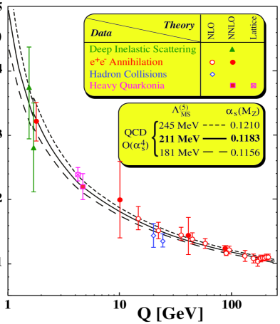
However, the deep inelastic scattering experiments showed slight deviation from Bjorken scaling, suggesting that the coupling of strong interactions was still not zero at any finite momentum transfer. This fit perfectly with the predictions of dependence of running coupling on an energy scale calculated from the renormalization group approach by Gross, Wilczek and Politzer. Later, more experiments were performed that confirmed this result. The dependence of the coupling on the energy scale and the experimental data are demonstrated in Fig. 1.

Figure 1: Summary of measurements of the running coupling of strong interactions $\alpha_{s}(Q)$ and its dependence on the energy scale [17].

Asymptotic freedom turned out to be a very useful property for studying high energy QCD. It allows one to treat the coupling constant perturbatively for sufficiently small distances and therefore calculate physical properties under consideration in a systematic and controlled manner.

The property of confinement is another interesting QCD phenomenon, it is discussed in the next section.

3 Confinement

Confinement is an important property of the strong interaction that is widely accepted and incorporated into any model claiming to imitate strong QCD. Being an essentially nonperturbative phenomenon, confinement still lacks a rigorous explanation from first principles despite more than 30 years of investigation.

Quark confinement is often defined as the absence of isolated quarks in nature as they have never been experimentally observed. Searches for free quarks normally focus on free particles with fractional electrical charge. But the observation of a particle with fractional charge does not necessarily mean that a free quark has been observed. For instance, there might exist heavy colored scalar particles that can form bound states with quarks producing massive states with fractional electric charge [18, 19].

Another definition of confinement is the physics phenomenon that color-charged particles cannot be isolated. But this confuses confinement with color screening, and also works for spontaneously broken gauge theories which are not supposed to exhibit confinement.

One can try to define confinement by its physical properties, for instance, the long range linear potential between quarks. However, this requirement is only reasonable for infinitely heavy quarks. When two quarks with finite masses become separated, at some point it becomes more energetically favorable for a new quark/anti-quark pair to be created out of the vacuum than to allow the quarks to separate further.

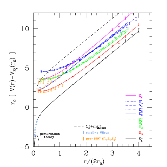
The lattice gauge approach has its own definition of confinement. Field theory is said to exhibit confinement if the interaction potential between quark and antiquark in this theory (which corresponds to the Wilson loop calculated on the lattice) has asymptotic linear behavior at large distances. Wilson loop measurements of various static quark potentials in the QCD vacuum are presented in Fig. 2. The lowest curve corresponds to the ground state of the gluonic field in the quark-antiquark system (meson) while higher curves correspond to the excited gluonic field (possibly hybrid states). One can see that for large distances all the potentials show linear behavior (confinement).

Figure 2: Wilson loop measurements of various static quark potentials [20].

Figure 3: Mesonic [22] and baryonic [21] flux tubes.

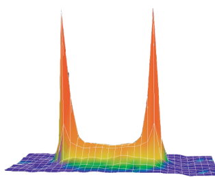
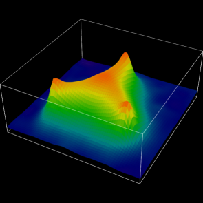
Gluonic fields can be visualized with the help of the plots of the action or gluonic field density made on the lattice (see Fig. 3 for meson (left) and baryon (right)). They clearly show that the quarks in a hadron are sources of color electric flux and that flux is trapped in a flux tube connecting the quarks. The formation of the flux tube is related to the self-interaction of gluons via their color charge. There exists a possibility that a gluonic field can be excited and, by interacting with quarks, produce mesons with exotic quantum numbers. Studying the spectrum of the exotic mesons one can learn a great deal about the structure of gluonic degrees of freedom and the confinement.

Since QCD is a gauge theory, it might be convenient to choose a specific gauge to study the particular property of the theory, such as confinement. It has been shown that the confinement of color charge could be easily understood in minimal Coulomb gauge, while, for instance, in Landau gauge the mechanism of this phenomenon is rather mysterious [23]. In minimal Coulomb gauge the 0-0 component of the gluon propagator,

$$D_{00}(x,t)=V_{coul}(x)\delta(t)+non\!-\!instantaneous,$$ (1)

has an instantaneous part, $V_{coul}(r)$, that is long range and confining and couples universally to all color-charge. The data of numerical study [24] are consistent with a linearly rising potential, $V_{coul}(r)\sim\sigma_{coul}r$, and a Coulomb string tension that is larger than the phenomenological string tension, $\sigma_{coul}>\sigma$. Moreover, the 3-dimensionally transverse physical components of the gluon propagator,

$$D_{ij}(x,t)=\langle A_{i}(x,t)A_{j}(0,0)\rangle,$$ (2)

are short range, corresponding to the absence of gluons from the physical spectrum. This property makes Coulomb gauge especially convenient to study nonperturbative QCD. More details on a study of confinement in Coulomb gauge can be found in [25]. The first serious look at Coulomb gauge and the problem of confinement there was in the paper by Szczepaniak and Swanson [26].

Every theory of confinement aims at explaining the linear rise of the static quark potential, which is suggested by the linearity of meson Regge trajectories. However, this phenomenon has a number of other interesting properties that a satisfactory theory of confinement is obligated to explain, one of them being Casimir scaling. Casimir scaling [27] refers to the fact that there is an intermediate range of distances where the string tension of static sources in color representation r is approximately proportional to the quadratic Casimir of the representation; i.e.

$$\sigma_{r}=\frac{C^{2}_{r}}{C^{2}_{F}}\sigma_{F},$$ (3)

where the subscript F refers to the fundamental representation. This behavior was first suggested in Ref. [28]. The term ‘Casimir scaling’ was introduced much later, in Ref. [27], where it was emphasized that this behavior poses a serious challenge to some prevailing ideas about confinement.

Figure 4: Casimir scaling of confinement [29].

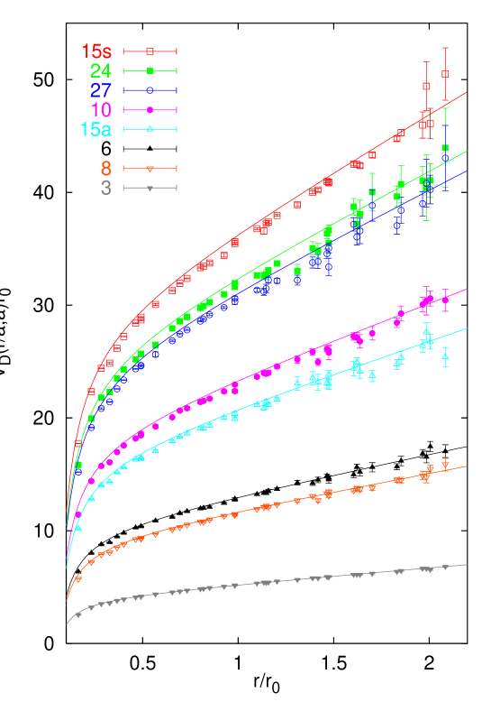
Figure 4 shows in a compelling way the property of Casimir scaling of confinement. The figure was obtained by measuring the Wilson loop for sources in various representations of SU(3). The interaction between color triplets is the lowest surface in the figure and forms the template for the others. In the figure one sees higher surfaces with sources in the 8, 6, $15_{A}$, 10, 27, 24, and $15_{S}$ representations. The curves are obtained by multiplying a fit to the lowest (fundamental representation) surface by the quadratic Casimir, $C^{2}_{r}=\langle r|T^{a}T^{a}|r\rangle$ divided by $C^{2}_{F}$. The quadratic Casimir is given by $(p^{2}+q^{2}+pq)/3+p+q$ where (p,q) is the Dynkin index of the representation. The agreement is remarkable and is a strong indication that the color structure of confinement may be modelled as

$$\int\bar{\psi}T^{a}\psi...\bar{\psi}T^{a}\psi$$ (4)

where the ellipsis represents Lorentz and spatial dependence.

Chiral symmetry breaking is another interesting QCD property, it is discussed in the next section.

4 Chiral symmetry breaking

In quantum field theory, chiral symmetry is a possible symmetry of the Lagrangian under which the left-handed and right-handed parts of Dirac fields transform independently. QCD Lagrangian has an approximate flavor chiral symmetry $SU_{L}(N_{f})\times SU_{R}(N_{f})$ due to the relative smallness of the masses of up, down and strange quarks. This approximate symmetry is dynamically broken to $SU(N_{f})$ and leads to the appearance of $(N_{f}^{2}-1)$ Goldstone bosons in the theory (which are pseudoscalar mesons for QCD). Since chiral symmetry is not exact (explicitly broken by small but nonzero quark masses), Goldstone bosons in QCD are not massless but relatively light. The actual masses of these mesons can in principle be obtained in chiral perturbation theory through an expansion in the (small) actual masses of the quarks.

The mechanism of dynamical chiral symmetry breaking is closely related to the structure of the vacuum. In QCD, quarks and antiquarks are strongly attracted to each other, therefore if these quarks are massless, the energy cost of the pair creation from the vacuum is small. So we expect that QCD vacuum contains quark-antiquark condensates with the vacuum quantum numbers (zero total momentum and angular momentum). It means that the condensates have nonzero chiral charge, pairing left-handed quarks with the antiparticles of right-handed quarks. It leads to the nonzero vacuum expectation value for the scalar operator

$$\langle 0|\bar{Q}Q|0\rangle=\langle 0|\bar{Q}_{L}Q_{R}+\bar{Q}_{R}Q_{L}|0\rangle\not{\!\!=}0.$$ (5)

The expectation value signals that the vacuum mixes the two quark helicities. This allows massless quarks to acquire effective mass as they move through the vacuum. Inside quark-antiquark bound states, quarks appear to move if they are massive, even though they have zero bare mass (in the Lagrangian).

Dynamical chiral symmetry breaking is impossible in perturbation theory because at every finite order in perturbation theory the self-energy of the particle is proportional to its renormalized mass. So if one starts with a chirally symmetric theory then one will also end up with a chirally symmetric theory, if using perturbative approaches. Therefore dynamical chiral symmetry breaking has to be studied using nonperturbative methods.

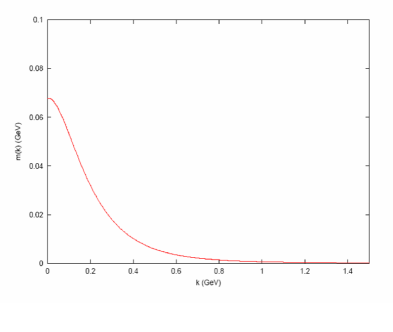
In the many-body approach dynamical chiral symmetry breaking and momentum-dependent mass generation of elementary excitations can be described by the Gap Equation (an example of a gap equation will be presented in section 2). The Gap Equation allows one to calculate the mass function of the particle which is momentum-dependent. The mass function of the quark calculated in this approach is presented in the Fig. 5. One can see that the dynamical quark mass is large in the infrared and suppressed in the ultraviolet, this result is not possible in weakly interacting theories.

Figure 5: Dependence of the dynamical quark mass on the momentum calculated in Coulomb gauge model introduced in section 2.

Another useful tool to study dynamical chiral symmetry breaking is the method based on Dyson-Schwinger equations. In fact, the simplest Dyson-Schwinger equation is the gap equation for the dressed quark propagator. By solving this equation one would obtain the mass function of the quark (dependence of the quark mass on the momentum). This equation cannot be solved exactly however since it is one of the equations of the self-consistent set of infinite number of coupled nonlinear integral equations. Truncation schemes appropriate to this problem have been found and the momentum-dependence of the quark mass has been calculated. It is in excellent agreement with lattice gauge theory calculations.

In the next chapter of the present dissertation we introduce the quark models studied and explain our methods.

Chapter 1 THEORY

The study of the meson sector has attracted much attention, with a great variety of different models. The fundamental reason is that it is a very good laboratory for exploring the nonperturbative QCD regime. ‘Composed of a quark and an antiquark’, a meson is the simplest nontrivial system that can be used to test basic QCD properties. In particular, the meson spectra can be reasonably understood in non-relativistic or semi-relativistic models with simple or sophisticated versions of the funnel potential, containing a long-range confining term plus a short-range Coulomb-type term coming from one-gluon exchange [30, 31].

Energies are not very stringent observables and to test more deeply the wave functions, one needs to rely on more sensitive observables. Electromagnetic properties, such as decay constants or form factors can be employed. In that case the transition operator is precisely known. On the other hand, one can also study hadronic transitions occurring through the strong interaction; this kind of transition is able to explain the decay of a meson into several mesons, or baryon-antibaryon, or other more complicated channels. The hadronization process is quite difficult to understand and model in terms of basic QCD. One reason is that, contrary to the electromagnetic case, the transition operator is not defined precisely.

1 Quark models of hadron structure

1 Nonrelativistic Potential Quark Model

In the nonrelativistic potential quark model the meson is approximated to be a bound state of interacting quark and antiquark. The meson state for such a system is:

$$|M\rangle = \sqrt{2E_{P}}\sum_{c\bar{c}s\bar{s}f\bar{f}M_{S}M_{L}}\frac{\delta_{c\bar{c}}}{\sqrt{3}}\langle JM|LM_{L}SM_{S}\rangle\chi^{SM_{S}}_{s\bar{s}}\,\Xi^{II_{z}}_{f\bar{f}}$$ (1)

$$\times\int\frac{d^{3}kd^{3}\bar{k}}{(2\pi)^{3}}\Phi\left(\frac{m_{\bar{q}}\vec{k}-m_{q}\vec{\bar{k}}}{m_{q}+m_{\bar{q}}}\right)\frac{\delta^{(3)}(\vec{k}+\vec{\bar{k}}-\vec{P})}{\sqrt{2E_{k}}\sqrt{2E_{\bar{k}}}}|\vec{k},\vec{\bar{k}}\rangle$$

where $\vec{P}$ is the meson momentum, $S$, $L$ and $J$ are the meson spin, orbital and angular momenta with projections $M_{S}$, $M_{L}$ and $M$. $X^{SM_{S}}_{s\bar{s}}$ is the spin wave function of the meson, it depends on spin projections of quark and antiquark $s$ and $\bar{s}$ and also on the meson spin and its projection. $\Xi^{II_{z}}_{f\bar{f}}$ is the flavor wave function and it depends on the flavors of the quark and antiquark $f$ and $\bar{f}$ and on the meson isospin $I$ and its projection $I_{z}$. $\Phi$ is the spatial wave function, it depends on the momenta $k$ and $\bar{k}$ of quark and antiquark with masses $m_{q}$ and $m_{\bar{q}}$.

In the nonrelativistic approximation the mesonic wave function is the eigenfunction of a Schrodinger equation:

$$\hat{H}\Psi=E\Psi,$$ (2)

and the Hamiltonian for the system is:

$$H=K+V(r),$$ (3)

where $K$ is the nonrelativistic kinetic energy and $V(r)$ is the potential energy.

Several phenomenological models for the interaction potential exist. The simplest one is a spherical harmonic oscillator potential. It is a rather crude approximation and doesn’t give good description of the meson properties, for example it can’t distinguish between two mesons with different spins. But it allows analytical calculations for most of the meson properties and easy Fourier transformations of the wave functions, so it is useful as a simple estimate of some physical quantities of interest.

Another variation of the nonrelativistic potential model is ISGW [32], which is based on SHO potential model but with an artificial factor $\kappa$ introduced so that $|\vec{q}|\rightarrow|\vec{q}|/\kappa$. The $\kappa$ factor was added to achieve better agreement with the experimental data for the pion form-factor and certain heavy quark transitions.

A more realistic model of the potential is Coulomb+linear+hyperfine interaction model:

$$V(r)=-\frac{4}{3}\frac{\alpha_{C}}{r}+br+C+\frac{32\alpha_{H}\sigma^{3}e^{-r^{2}\sigma^{2}}}{9m_{1}m_{2}\pi^{1/2}}\,\vec{S}_{1}\cdot\vec{S}_{2}.$$ (4)

The strengths of the Coulomb and hyperfine interactions are taken as separate parameters. Perturbative gluon exchange implies that $\alpha_{C}=\alpha_{H}$ and we find that the fits prefer the near equality of these parameters.

The Coulomb term corresponds to the quark interaction due to the one gluon exchange and dominates at short range. The linear term describes confinement. The hyperfine term is spin-dependent and makes it possible to distinguish between mesons of different spins. This potential has 3 parameters ($\alpha$, $\beta$ and $\sigma$), and together with the mass of the quarks they could be adjusted to describe the properties of the mesons (for examples the masses of several meson ground states). After the parameters have been adjusted, calculations of other meson properties could be done and compared to the experimental data to see how the model works. Also predictions of the physical properties, potentially observable in the future, could be made.

As will be described in the next chapter, the observables that we consider require a weaker ultraviolet interaction than that of Eq. 4. We therefore introduce a running coupling that recovers the perturbative coupling of QCD but saturates at a phenomenological value at low momenta:

$$\alpha_{C}\to\alpha_{C}(k)=\frac{4\pi}{\beta_{0}\log\left({e^{\frac{4\pi}{\beta_{0}\alpha_{0}}}+\frac{k^{2}}{\Lambda^{2}}}\right)}$$ (5)

where $k^{2}=|\vec{k}|^{2}$ is the square of the three-momentum transfer, $\beta_{0}=11-2N_{f}/3=9$, $N_{f}$ is the number of flavors taken to be 3. One can identify the parameter $\Lambda$ with $\Lambda_{QCD}$ because $\alpha_{C}(k)$ approaches the one loop running constant of QCD. However, this parameter will also be fit to experimental data in the following (nevertheless, the resulting preferred value is reassuringly close to expectations). Parameters and details of the fit are presented in the Chapter 3.

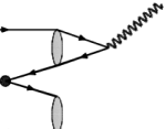
Potential of Eq. 4 cannot explain P-wave mass splittings induced by spin-dependent interactions, which are due to spin-orbit and tensor terms. A common model of spin-dependence is based on the Breit-Fermi reduction of the one-gluon-exchange interaction supplemented with the spin-dependence due to a scalar current confinement interaction. The general form of this potential has been computed by Eichten and Feinberg[33] at tree level using Wilson loop methodology. The result is parameterized in terms of four nonperturbative matrix elements, $V_{i}$, which can be determined by electric and magnetic field insertions on quark lines in the Wilson loop. Subsequently, Pantaleone, Tye, and Ng[34] performed in a one-loop computation of the heavy quark interaction and showed that a fifth interaction, $V_{5}$ is present in the case of unequal quark masses. The diagrams that have been calculated in addition to the tree level diagram are presented in Fig. 1.

Figure 1: One-loop diagrams of the heavy quark interaction.

The net result is a quark-antiquark interaction that can be written as:

$$V_{q\bar{q}}=V_{conf}+V_{SD}$$ (6)

where $V_{conf}$ is the standard Coulomb+linear scalar form:

$$V_{conf}(r)=-\frac{4}{3}\frac{\alpha_{s}}{r}+br$$ (7)

and

$$V_{SD}(r) = \left({\bm{\sigma}_{q}\over 4m_{q}^{2}}+{\bm{\sigma}_{\bar{q}}\over 4m_{\bar{q}}^{2}}\right)\cdot{\bf L}\left({1\over r}{dV_{conf}\over dr}+{2\over r}{dV_{1}\over dr}\right)+\left({\bm{\sigma}_{\bar{q}}+\bm{\sigma}_{q}\over 2m_{q}m_{\bar{q}}}\right)\cdot{\bf L}\left({1\over r}{dV_{2}\over dr}\right)$$ (8)

$$+{1\over 12m_{q}m_{\bar{q}}}\Big{(}3\bm{\sigma}_{q}\cdot\hat{\bf r}\,\bm{\sigma}_{\bar{q}}\cdot\hat{\bf r}-\bm{\sigma}_{q}\cdot\bm{\sigma}_{\bar{q}}\Big{)}V_{3}+{1\over 12m_{q}m_{\bar{q}}}\bm{\sigma}_{q}\cdot\bm{\sigma}_{\bar{q}}V_{4}$$

$$+{1\over 2}\left[\left({\bm{\sigma}_{q}\over m_{q}^{2}}-{\bm{\sigma}_{\bar{q}}\over m_{\bar{q}}^{2}}\right)\cdot{\bf L}+\left({\bm{\sigma}_{q}-\bm{\sigma}_{\bar{q}}\over m_{q}m_{\bar{q}}}\right)\cdot{\bf L}\right]V_{5}.$$

Here ${\bf L}={\bf L}_{q}=-{\bf L_{\bar{q}}}$, $r=|{\bf r}|=|{\bf r}_{q}-{\bf r}_{\bar{q}}|$ is the ${\bar{Q}Q}$ separation and the $V_{i}=V_{i}(m_{q},m_{\bar{q}};r)$ are the Wilson loop matrix elements discussed above. The explicit expressions for $V_{i}$’s can be found in the section 3 of the present dissertation.

The first four $V_{i}$ are order $\alpha_{s}$ in perturbation theory, while $V_{5}$ is order $\alpha_{s}^{2}$; for this reason $V_{5}$ has been ignored by quark modelers. For example, the analysis of Cahn and Jackson[35] only considers $V_{1}$ – $V_{4}$. In practice this is acceptable (as we show later) except in the case of unequal quark masses, where the additional spin-orbit interaction can play an important role.

2 Relativistic Many-Body Approach in Coulomb Gauge

The canonical nonrelativistic quark model relies on a potential description of quark dynamics and therefore neglects many-body effects in QCD. Related to this is the question of the reliability of nonrelativistic approximations, the importance of hadronic decays, and the chiral nature of the pion. The latter two phenomena depend on the behavior of nonperturbative glue and as such are crucial to the development of robust models of QCD and to understanding soft gluodynamics. Certainly, one expects that gluodynamics will make its presence felt with increasing insistence as experiments probe higher excitations in the spectrum. Similarly the chiral nature of the pion cannot be understood in a fixed particle number formalism. This additional complexity is the reason so few models attempt to derive the chiral properties of the pion. This is an unfortunate situation since the pion is central to much of hadronic and nuclear physics.

To make progress one must either resort to numerical experiments or construct models which are closer to QCD. One such model is based on the QCD Hamiltonian in Coulomb gauge [36, 37, 38, 40].

In this approach the exact QCD Hamiltonian in the Coulomb gauge is modeled by an effective, confining Hamiltonian, that is relativistic with quark field operators and current quark masses. However, before approximately diagonalizing H, a similarity transformation is implemented to a new quasiparticle basis having a dressed, but unknown constituent mass. As described later, this transformation entails a rotation that mixes the bare quark creation and annihilation operators. By then performing a variational calculation to minimize the ground state (vacuum) energy, a specific mixing angle and corresponding quasiparticle mass is selected. In this fashion chiral symmetry is dynamically broken and a non-trivial vacuum with quark condensates emerges. This treatment is precisely analogous to the Bardeen, Cooper, and Schrieffer (BCS) description of a superconducting metal as a coherent vacuum state of interacting quasiparticles combining to form condensates (Cooper pairs). Excited states (mesons) can then be represented as quasiparticle excitations using standard many-body techniques, for example Tamm-Dancoff (TDA) or random phase approximation (RPA) methods.

There are several reasons for choosing the Coulomb gauge framework. As discussed by Zwanziger [39], the Hamiltonian is renormalizable in this gauge and, equally as important, the Gribov problem ($\Delta\cdot A=0$ does not uniquely specify the gauge) can be resolved (see Refs. [ZW, 40] for further discussion). Related, there are no spurious gluon degrees of freedom since only transverse gluons enter. This ensures all Hilbert vectors have positive normalizations which is essential for using variational techniques that have been widely successful in atomic, molecular and condensed matter physics. Second, an advantage of Coulomb gauge is the appearance of an instantaneous potential.

By introducing a potential $K^{(0)}$, the QCD Coulomb gauge Hamiltonian [40] for the quark sector can be replaced by an effective Hamiltonian

$$H=\int d\vec{x}\bar{\Psi}^{{\dagger}}\left(\vec{x}\right)\left(-i\vec{\alpha}\cdot\vec{\Delta}+\beta m\right)\bar{\Psi}\left(\vec{x}\right)+\frac{1}{2}\int d\vec{x}d\vec{y}\rho^{a}\left(\vec{x}\right)K^{(0)}\left(|\vec{x}-\vec{y}|\right)\rho^{a}\left(\vec{y}\right),$$ (9)

where $\Psi$, $m$ and $\rho^{a}(\vec{x})=\Psi^{{\dagger}}\left(\vec{x}\right)T^{a}\Psi\left(\vec{x}\right)$ are the current (bare) quark field, mass and color density, respectively. For notational ease the flavor subscript is omitted (same H for each flavor) and the color index runs $a=1...8$.

$K^{(0)}$ is defined as the vacuum expectation value of the instantaneous non-Abelian Coulomb interaction. The procedure for calculating $K^{(0)}$ is described in [26]. The solution is well approximated by the following expression:

$$K^{(0)}(k)=\frac{12.25}{k^{2}}\left\{\begin{array}[]{lc}\left(\frac{m_{g}}{k}\right)^{1.93}&k<m_{g},\\ 0.6588\log{(k^{2}/m^{2}_{g}+0.82)}^{-0.62}\log{(k^{2}/m^{2}_{g}+1.41)}^{-0.80}&k>m_{g}.\end{array}\right.$$ (12)

To find the meson wave function, equation $H\Psi=E\Psi$ has to be solved as accurately as possible. First the ground state has to be studied, and the Bogoliubov-Valatin, or BCS, transformation is introduced.

The plane wave, spinor expansion for the quark field operator is:

$$\Psi(\vec{x})=\sum_{c\lambda}\int\frac{d\vec{k}}{(2\pi)^{3}}\left[u_{c\lambda}(\vec{k})b_{c\lambda}(\vec{k})+v_{c\lambda}(-\vec{k})d^{{\dagger}}_{c\lambda}(-\vec{k})\right]e^{i\vec{k}\cdot\vec{x}}$$ (13)

with free particle, anti-particle spinors $u_{c\lambda}$, $v_{c\lambda}$ and bare creation, annihilation operators $b_{c\lambda}$, $d_{c\lambda}$ for current quarks, respectively. Here the spin state (helicity) is denoted by $\lambda$ and color index by $c=1,2,3$ (which is hereafter suppressed). Because $\Psi$ could be expanded in terms of any complete basis, a new quasiparticle basis may equally well be used:

$$\Psi(\vec{x})=\sum_{\lambda}\int\frac{d\vec{k}}{(2\pi)^{3}}\left[U_{\lambda}(\vec{k})B_{\lambda}(\vec{k})+V_{\lambda}(-\vec{k})D^{{\dagger}}_{\lambda}(-\vec{k})\right]e^{i\vec{k}\cdot\vec{x}}$$ (14)

entailing quasiparticle spinors $U_{\lambda}$, $V_{\lambda}$ and operators $B_{\lambda}$,$D_{\lambda}$. The Hamiltonian is equivalent in either basis and the two are related by a similarity (Bogoliubov-Valatin or BCS) transformation. The transformation between operators is given by the rotation

$$B_{\lambda}(\vec{k})=\cos{\frac{\theta_{k}}{2}}b_{\lambda}(\vec{k})-\lambda\sin{\frac{\theta_{k}}{2}}d^{{\dagger}}_{\lambda}(-\vec{k}),$$

$$D_{\lambda}(-\vec{k})=\cos{\frac{\theta_{k}}{2}}d_{\lambda}(-\vec{k})+\lambda\sin{\frac{\theta_{k}}{2}}b^{{\dagger}}_{\lambda}(\vec{k}),$$ (15)

involving the BCS angle $\theta_{k}=\theta(k)$. Similarly the rotated quasiparticle spinors are

$$U_{\lambda}(\vec{k})=\cos{\frac{\theta_{k}}{2}}u_{\lambda}(\vec{k})-\lambda\sin{\frac{\theta_{k}}{2}}v_{\lambda}(-\vec{k})=\frac{1}{\sqrt{2}}\left[\begin{array}[]{c}\sqrt{1+\sin{\phi(\vec{k})}}\,\,\,\chi_{\lambda}\\ \sqrt{1-\sin{\phi(\vec{k})}}\,\,\,\vec{\sigma}\cdot\hat{k}\,\,\,\chi_{\lambda}\end{array}\right],$$ (18)

$$V_{\lambda}(-\vec{k})=\cos{\frac{\theta_{k}}{2}}v_{\lambda}(-\vec{k})+\lambda\sin{\frac{\theta_{k}}{2}}u_{\lambda}(\vec{k})=\frac{1}{\sqrt{2}}\left[\begin{array}[]{c}-\sqrt{1-\sin{\phi(\vec{k})}}\,\,\,\vec{\sigma}\cdot\hat{k}\,\,\,\chi_{\lambda}\\ \sqrt{1+\sin{\phi(\vec{k})}}\,\,\,\chi_{\lambda}\end{array}\right],$$ (21)

where $\chi_{\lambda}$ is the standard two-dimensional Pauli spinor. The gap angle, $\phi_{k}=\phi(k)$, has also been introduced, which is related to the BCS angle, $\theta/2$, by $\phi=\theta+\alpha$ where $\alpha$ is the current, or perturbative, mass angle satisfying $\sin{\alpha}=m/E_{k}$ with $E_{k}=\sqrt{m^{2}+k^{2}}$. Hence

$$\sin{\phi_{k}}=\frac{m}{E_{k}}\cos{\theta_{k}}+\frac{k}{E_{k}}\sin{\theta_{k}},$$

$$\cos{\phi_{k}}=\frac{k}{E_{k}}\cos{\theta_{k}}-\frac{m}{E_{k}}\sin{\theta_{k}}.$$ (22)

Similarly, the perturbative, trivial vacuum, defined by $b_{\lambda}|0\rangle=d_{\lambda}|0\rangle=0$, is related to the quasiparticle vacuum, $B_{\lambda}|\Omega\rangle=D_{\lambda}|\Omega\rangle=0$, by the transformation

$$|\Omega\rangle=exp\left(-\sum_{\lambda}\int\frac{d\vec{k}}{(2\pi)^{3}}\lambda\tan{\frac{\theta_{k}}{2}}b^{{\dagger}}_{\lambda}(\vec{k})d^{{\dagger}}_{\lambda}(-\vec{k})\right)|0\rangle.$$ (23)

Here $\Omega$ is so called BCS vacuum (later we introduce the RPA vacuum labeled $|\Omega_{RPA}\rangle$ which is required to obtain a massless pion). Expanding the exponential and noting that the form of the operator $b^{{\dagger}}d^{{\dagger}}$ is designed to create a current quark/antiquark pair with the vacuum quantum numbers, clearly exhibits the BCS vacuum as a coherent state of quark/antiquark excitations (Cooper pairs) representing ${}^{2S+1}L_{J}=\,^{3}P_{0}$ condensates. One can regard $tan{\frac{\theta_{k}}{2}}$ as the momentum wavefunction of the pair in the center of momentum system.

An approximate ground state for our effective Hamiltonian could be found by minimizing the BCS vacuum expectation, $\langle\Omega|H|\Omega\rangle$. It could be done variationally using the gap angle, $\phi_{k}$, which leads to the gap equation, $\delta\langle\Omega|H|\Omega\rangle=0$. After considerable mathematical reduction, the nonlinear integral gap equation follows

$$k\sin{\phi_{k}}-m\cos{\phi_{k}}=\frac{2}{3}\int\frac{d\vec{q}}{(2\pi)^{3}}K^{(0)}\left(|\vec{k}-\vec{q}|\right)\left[\sin{\phi_{k}}\cos{\phi_{q}}\hat{k}\cdot\hat{q}-\sin{\phi_{q}}\cos{\phi_{k}}\right].$$ (24)

This gap equation is to be solved for the unknown Bogoliubov angle, which then specifies the quark vacuum and the quark field mode expansion via spinors. Comparing the quark spinor to the canonical spinor permits a simple interpretation of the Bogoliubov angle through the relationship $\mu(k)=k\tan{\phi_{k}}$ where $\mu(k)$ may be interpreted as a dynamical momentum-dependent quark mass. Similarly $\mu(0)$ may be interpreted as a constituent quark mass.

The numerical solution for the dynamical quark mass is very accurately represented by the functional form

$$\mu(k)=\sigma K^{(0)}(k)\left(1-e^{-M/(\sigma K^{(0)})(k)}\right)$$ (25)

where M is a constituent quark mass and $\sigma$ is a parameter related to the quark condensate. Notice that this form approaches the constituent mass for small momenta and $\sigma K^{(0)}$ for large momenta.

With explicit expressions for the quark interaction and the dynamical quark mass the mesonic bound states can now be obtained. The definitions of the meson creation operators in TDA and RPA approximations are (see $\S 59$ of Ref. [41], also [42, 43]):

$$Q^{{\dagger}}_{M}(TDA) = \sum_{\gamma\delta}\int\frac{d^{3}k}{(2\pi)^{3}}\psi_{\gamma\delta}(\vec{k})B^{{\dagger}}_{\gamma}(\vec{k})D^{{\dagger}}_{\delta}(-\vec{k}),$$ (26)

$$Q^{{\dagger}}_{M}(RPA) = \sum_{\gamma\delta}\int\frac{d^{3}k}{(2\pi)^{3}}\left[\psi^{{\dagger}}_{\gamma\delta}(\vec{k})B^{{\dagger}}_{\gamma}(\vec{k})D^{{\dagger}}_{\delta}(-\vec{k})-\psi^{-}_{\gamma\delta}(\vec{k})B_{\gamma}(\vec{k})D_{\delta}(-\vec{k})\right]$$ (27)

with $B$ and $D$ being the quasiparticle operators. It is worthwhile recalling that the RPA method is equivalent to the Bethe-Salpeter approach with instantaneous interactions [44].

A meson is then represented by the Fock space expansion:

$$|M_{TDA}\rangle = Q^{{\dagger}}_{M}(TDA)|\Omega\rangle,$$ (28)

$$|M_{RPA}\rangle = Q^{{\dagger}}_{M}(RPA)|\Omega_{RPA}\rangle.$$ (29)

Here $\Omega_{RPA}$ is RPA vacuum, it has both fermion (two quasiparticles or Cooper pairs) and boson (four quasiparticles or meson pairs) correlations.

To derive the TDA and RPA equations of motion we project the Hamiltonian equation onto the truncated Fock sector. It gives:

$$\langle M_{TDA}|[H,Q^{{\dagger}}_{M}(TDA)]|\Omega\rangle=(E_{M}-E_{0})\langle M_{TDA}|Q^{{\dagger}}_{M}(TDA)|\Omega\rangle,$$ (30)

$$\langle M_{RPA}|[H,Q^{{\dagger}}_{M}(RPA)]|\Omega_{RPA}\rangle=(E_{M}-E_{0})\langle M_{RPA}|Q^{{\dagger}}_{M}(RPA)|\Omega_{RPA}\rangle$$ (31)

In TDA (30) generates an integral equation for the meson wave function $\psi(\vec{k})$, and in RPA (31) generates two coupled nonlinear integral equations for two wave functions $\psi^{{\dagger}}(\vec{k})$ and $\psi^{-}(\vec{k})$.

The RPA and TDA equations include self energy terms (denoted $\Sigma$) for each quark line and these must be renormalized. In the zero quark mass case renormalization of the TDA or RPA equations proceeds in the same way as for the quark gap equation. In fact, the renormalization of these equations is consistent and one may show that a finite gap equation implies a finite RPA or TDA equation. This feature remains true in the massive case. The RPA equation in the pion channel reads:

$$(E_{\pi}-E_{BCS})\psi^{{\dagger}}(k) = 2\left[m\sin{\phi_{k}}+k\cos{\phi_{k}}+\Sigma(k)\right]\psi^{{\dagger}}(k)-$$

$$-\frac{C_{F}}{2}\int\frac{q^{2}dq}{(2\pi)^{3}}\Big{[}V_{0}(k,q)(1+\sin{\phi_{k}}\sin{\phi_{q}})+V_{1}(k,p)\cos{\phi_{k}}\cos{\phi_{q}}\Big{]}\psi^{{\dagger}}(q)-$$

$$-\frac{C_{F}}{2}\int\frac{q^{2}dq}{(2\pi)^{3}}\Big{[}V_{0}(k,q)(1-\sin{\phi_{k}}\sin{\phi_{q}})-V_{1}(k,p)\cos{\phi_{k}}\cos{\phi_{q}}\Big{]}\psi^{-}(q),$$

where

$$V_{L}(k,q)=2\pi\int d(\hat{q}\cdot\hat{k})K^{(0)}\left(|\vec{q}-\vec{k}|\right)P_{L}(\hat{q}\cdot\hat{k}).$$ (33)

A similar equation for $\psi^{-}$ holds with $(+\rightarrow-)$ and $E\rightarrow-E$. The wavefunctions $\psi^{\pm}$ represent forward and backward moving components of the many-body wavefunction and the pion itself is a collective excitation with infinitely many constituent quarks in the Fock space expansion. These two coupled nonlinear integral equation could be solved numerically to obtain meson spectrum and wave functions.

TDA equation may be obtained from the RPA equation (2) by neglecting the backward wave function $\psi^{-}$. The spectrum in the random phase and Tamm-Dancoff approximations has been computed [45] and it has been confirmed that the pion is massless in the chiral limit. It was also found that the Tamm-Dancoff approximation yields results very close to the RPA for all states except the pion. All other mesons have nearly identical RPA and TDA masses. The complete hidden flavor meson spectrum in the Tamm-Dancoff approximation is given by the following equations.

$$E\psi_{PC}(k)=2\left[m\sin{\phi_{k}}+k\cos{\phi_{k}}+\Sigma(k)\right]\psi_{PC}(k)-\frac{C_{F}}{2}\int\frac{q^{2}dq}{(2\pi)^{3}}K^{PC}_{J}(k,q)\psi_{PC}(q)$$ (34)

with

$$\Sigma(k)=\frac{C_{F}}{2}\int\frac{q^{2}dq}{(2\pi)^{3}}\left(V_{0}\sin{\phi_{k}}\sin{\phi_{q}}+V_{1}\cos{\phi_{k}}\cos{\phi_{q}}\right)$$ (35)

and where $\psi$ is the meson radial wavefunction in momentum space. Note that the imaginary part of the self-energy $Im(\Sigma)=0$, this follows from the fact that the quark-antiquark interaction is instantaneous in the Coulomb gauge.

The kernel $K_{J}$ in the potential term depends on the meson quantum numbers, $J^{PC}$. In the following possible values for the parity or charge conjugation eigenvalues are denoted by $(J)=+$ if $J$ is even and $-$ if $J$ is odd. These interaction kernels have been derived in the quark helicity basis (see for example Ref. [45]).

• $0^{++}$
  

  $$K(p,k)=V_{0}\cos{\phi_{p}}\cos{\phi_{k}}+V_{1}\left(1+\sin{\phi_{p}}\sin{\phi_{k}}\right)$$ (36)

• $J^{(J+1)(J)}\,\,\,\,[^{1}J_{J},J\geq 0]$
  

  $$K_{J}(p,k)=V_{J}\left(1+\sin{\phi_{p}}\sin{\phi_{k}}\right)+\left(V_{J-1}\frac{J}{2J+1}+V_{J+1}\frac{J+1}{2J+1}\right)\cos{\phi_{p}}\cos{\phi_{k}}$$ (37)

• $J^{(J+1)(J+1)}\,\,\,\,[^{3}J_{J},J\geq 1]$
  

  $$K_{J}(p,k)=V_{J}\left(1+\sin{\phi_{p}}\sin{\phi_{k}}\right)+\left(V_{J-1}\frac{J+1}{2J+1}+V_{J+1}\frac{J}{2J+1}\right)\cos{\phi_{p}}\cos{\phi_{k}}$$ (38)

• $J^{(J)(J)}\,\,\,\,[^{3}(J-1)_{J},^{3}(J+1)_{J},J\geq 1]$

  $$K_{11}(p,k) = V_{J}\cos{\phi_{p}}\cos{\phi_{k}}+\left(V_{J-1}\frac{J}{2J+1}+V_{J+1}\frac{J+1}{2J+1}\right)\left(1+\sin{\phi_{p}}\sin{\phi_{k}}\right)$$

  $$K_{22}(p,k) = V_{J}\cos{\phi_{p}}\cos{\phi_{k}}+\left(V_{J-1}\frac{J+1}{2J+1}+V_{J+1}\frac{J}{2J+1}\right)\left(1+\sin{\phi_{p}}\sin{\phi_{k}}\right)$$

  $$K_{12}(p,k) = \left(V_{J-1}-V_{J+1}\right)\frac{\sqrt{J(J+1)}}{2J+1}\left(\sin{\phi_{k}}+\sin{\phi_{p}}\right)$$ (39)

2 Strong decays

The decay of a meson into two mesons is the simplest example of a strong decay. The decay of a baryon into a meson and a baryon has also been extensively studied. Even in those particularly simple decays, various models have been proposed to explain the mechanism. Among them, let us cite the naive $SU(6)_{W}$ model [46], the elementary meson-emission model [47, 48, 49, 50, 51] (in which one emitted meson is considered as an elementary particle coupled to the quark), the ${}^{3}S_{1}$ model [52, 53] (in which a quark-antiquark pair is created from the gluon emitted by a quark of the original meson), the flux-tube model [54] and the ${}^{3}P_{0}$ model (in which a quark-antiquark pair is created from the vacuum) [55, 56, 57, 58].

This last model (${}^{3}P_{0}$) is especially attractive because it can provide the gross features of various transitions with only one parameter, the constant corresponding to the creation vertex. This property is of course an oversimplification because there is no serious foundation for a creation vertex independent of the momenta of the created quarks. Even in the ${}^{3}P_{0}$ model, the form of the vertex is essentially unknown.

This phenomenological model of hadron decays was developed in the 1970s by LeYaouanc et al, [56], which assumes, as suggested earlier by Micu in [55], that during a hadron decay a $q\bar{q}$ pair is produced from the vacuum with vacuum quantum numbers, $J^{PC}=0^{++}$. Since this corresponds to a ${}^{3}P_{0}$ $q\bar{q}$ state, this is now generally referred to as the ${}^{3}P_{0}$ decay model. The ${}^{3}P_{0}$ pair production Hamiltonian for the decay of a $q\bar{q}$ meson A to mesons B + C is usually written in a rather complicated form with explicit wavefunctions [59], which in the conventions of Geiger and Swanson [60] (to within an irrelevant overall phase) is

$$\langle BC|H_{I}|A\rangle=\gamma\int\int\frac{d^{3}rd^{3}y}{(2\pi)^{3/2}}e^{\frac{i}{2}\vec{P}_{B}\cdot\vec{r}}\Psi_{A}\left(\vec{r}\right)\langle\vec{\sigma}\rangle_{q\bar{q}}\cdot\left(i\vec{\Delta}_{B}+i\vec{\Delta}_{C}\right. \!\!\!\!\!\!\!\!\left.+\vec{P}_{B}\right)\Psi^{*}_{B}\left(\frac{\vec{r}}{2}+\vec{y}\right)\Psi^{*}_{C}\left(\frac{\vec{r}}{2}-\vec{y}\right)$$ (40)

$$\delta\left(\vec{P}_{A}-\vec{P}_{B}-\vec{P}_{C}\right)$$

for all quark and antiquark masses equal. The strength $\gamma$ of the decay interaction is regarded as a free constant and is fitted to data [61].

Studies of hadron decays using this model have been concerned almost exclusively with numerical predictions, and have not led to any fundamental modifications. Recent studies have considered changes in the spatial dependence of the pair production amplitude as a function of quark coordinates [59] but the fundamental decay mechanism is usually not addressed; this is widely believed to be a nonperturbative process, involving flux tube breaking .

3 Electromagnetic and electroweak transitions

Since the operator of electromagnetic and electroweak transitions is very well known, studying these processes for hadrons could provide us with valuable information on the hadron structure. Still these transitions are complicated enough, so that simplifying approximations are typically in use. In this section, different types of electromagnetic and electroweak transitions are described, and approaches to study them are explained.

1 Decay constants

Leptonic decay constants are a simple probe of the short distance structure of hadrons and therefore are a useful observable for testing quark dynamics in this regime. Decay constants are computed by equating their field theoretic definition with the analogous quark model definition. This identification is rigorously valid in the nonrelativistic and weak binding limits where quark model state vectors form good representations of the Lorentz group[32, 63]. The task at hand is to determine the reliability of the computation away from these limits.

The method is illustrated with the vector meson decay constant $f_{V}$, which is defined by

$$m_{V}\,f_{V}\,\epsilon^{\mu}=\langle 0|\bar{\Psi}(0)\gamma^{\mu}\Psi(0)|V\rangle$$ (41)

where $m_{V}$ is the vector meson mass and $\epsilon^{\mu}$ is its polarization vector. Note that the vector current is locally conserved for the physical vector meson.

The decay constant is computed in the conceptual weak binding and nonrelativistic limit of the quark model and is assumed to be accurate away from these limits. One thus employs the quark model state:

$$|V(P)\rangle=\sqrt{\frac{2E_{P}}{N_{c}}}\chi^{SM_{S}}_{s\bar{s}}\,\int\frac{d^{3}k\,d^{3}\bar{k}}{(2\pi)^{3}}\Phi\left(\frac{m_{\bar{q}}\vec{k}-m_{q}\vec{\bar{k}}}{m_{\bar{q}}+m_{q}}\right)\delta^{(3)}(\vec{k}+\vec{\bar{k}}-\vec{P})b^{\dagger}_{ks}d^{\dagger}_{\bar{k}\bar{s}}|0\rangle,$$ (42)

where $m_{q}$ and $m_{\bar{q}}$ are the masses of quark and antiquark with momenta $\vec{k}$ and $\vec{\bar{k}}$ accordingly, $\vec{P}$ is the vector meson momentum. The decay constant is obtained by computing the spatial matrix element of the current in the vector center of mass frame (the temporal component is trivial) and yields

$$f_{V}=\sqrt{\frac{N_{c}}{m_{V}}}\int\frac{d^{3}k}{(2\pi)^{3}}\Phi(\vec{k})\sqrt{1+\frac{m_{q}}{E_{k}}}\sqrt{1+\frac{m_{\bar{q}}}{E_{\bar{k}}}}\left(1+\frac{k^{2}}{3(E_{k}+m_{q})(E_{\bar{k}}+m_{\bar{q}})}\right).$$ (43)

The nonrelativistic limit is proportional to the meson wave function at the origin

$$f_{V}=2\sqrt{\frac{N_{c}}{m_{V}}}\tilde{\Phi}(r=0);$$ (44)

which recovers the well-known result of van Royen and Weisskopf[64].

Decay constant for vector mesons with quark and antiquark of the same flavor could be determined from the experimental data for the decay $V\rightarrow e^{+}e^{-}$. In this process the vector meson first converts into the photon and then photon becomes the electron-positron pair. The amplitude of this process is then:

$$A_{s_{1}s_{2}}=\langle e^{+}e^{-}|\bar{\Psi}\gamma^{\mu}\Psi|0\rangle\langle 0|\bar{\Psi}\gamma_{\mu}\Psi|V\rangle=\frac{e^{2}}{q^{2}}Q\bar{u}_{s_{1}}(p_{1})\gamma^{\mu}v_{s_{2}}(p_{2})f_{V}m_{V}\epsilon_{\mu}$$ (45)

where $p_{1}$ and $p_{2}$ are the momenta, $s_{1}$ and $s_{2}$ are spins of the electron and positron, Q is the quark charge (in units of $e$), $q$ is the photon momentum.

Then the squared amplitude summed over the electron and positron spins and averaged over vector meson polarizations is:

$$|A|^{2}=\frac{1}{3}\sum_{s_{1}s_{2}}|A_{s_{1}s_{2}}|^{2} = \frac{e^{4}}{3q^{4}}Q^{2}f^{2}_{V}m^{2}_{V}\epsilon_{\mu}\epsilon^{*}_{\nu}\sum_{s_{1}s_{2}}\left[\bar{u}_{s_{1}}(p_{1})\gamma^{\mu}v_{s_{2}}(p_{2})\bar{v}_{s_{2}}(p_{2})\gamma^{\nu}u_{s_{1}}(p_{1})\right]$$ (46)

$$= \frac{e^{4}}{3q^{4}}Q^{2}f^{2}_{V}m^{2}_{V}(-g_{\mu\nu})Tr[(\hbox to0.0pt{/\hss}{p_{2}}-m_{e})\gamma^{\nu}(\hbox to0.0pt{/\hss}{p_{1}}+m_{e})\gamma^{\mu}]$$

$$= -\frac{4e^{4}}{3q^{4}}Q^{2}f^{2}_{V}m^{2}_{V}g_{\mu\nu}[p^{\nu}_{2}p^{\mu}_{1}+p^{\nu}_{1}p^{\mu}_{2}-g^{\mu\nu}(p_{1}\cdot p_{2}+m^{2}_{e})]$$

Since in this process the masses of electron and positron are much smaller than their momenta, we can neglect $m_{e}$. Then:

$$|A|^{2}=\frac{8e^{4}}{3q^{4}}Q^{2}f^{2}_{V}m^{2}_{V}(p_{1}\cdot p_{2})$$ (47)

From the momentum conservation law $q=p_{1}+p_{2}$ so

$$(p_{1}+p_{2})^{2}=p^{2}_{1}+p^{2}_{2}+2p_{1}p_{2}=2m^{2}_{e}+2p_{1}p_{2}\approx 2p_{1}p_{2}=q^{2}$$ (48)

and then $p_{1}p_{2}=q^{2}/2$ so

$$|A|^{2}=\frac{4e^{4}}{3q^{2}}Q^{2}f^{2}_{V}m^{2}_{V}=\frac{4}{3}e^{4}Q^{2}f^{2}_{V}$$ (49)

because in the meson rest frame $q=m_{V}$.

Now we can calculate the decay rate of this process:

$$\Gamma_{V\rightarrow e^{+}e^{-}}=\frac{1}{2m_{V}}\int\frac{d\Omega_{cm}}{32\pi^{2}}\left(\frac{2|\vec{p}_{1}|}{E_{cm}}\right)|A|^{2}$$ (50)

Here $E_{cm}$ is the energy of the final state in its rest frame. Since $m_{e}\approx 0$ then $E_{cm}=2|\vec{p}_{1}|$ and then the decay rate is:

$$\Gamma_{V\rightarrow e^{+}e^{-}}=\frac{e^{4}Q^{2}f^{2}_{V}}{12\pi m_{V}}=\frac{4\pi\alpha^{2}}{3}\frac{Q^{2}f^{2}_{V}}{m_{V}}$$ (51)

and the decay constant is:

$$f_{V}=\left(\frac{3m_{V}\Gamma_{V\rightarrow e^{+}e^{-}}}{4\pi\alpha^{2}Q^{2}}\right)^{1/2}$$ (52)

That gives the following results for the existing vector mesons:

$$f_{\rho}=217MeV (Q=\frac{1}{\sqrt{2}})$$

$$f_{\phi}=229MeV (Q=-\frac{1}{3})$$

$$f_{J/\psi}=411MeV (Q=\frac{2}{3})$$

$$f_{\Upsilon}=704MeV (Q=-\frac{1}{3})$$ (53)

Similar results hold for other mesons that couple to electroweak currents. A summary of the results for a variety of models and the discussion are presented in Chapter 3. The expressions used to compute the table entries and the data used to extract the experimental decay constants are collected in Appendix 8.

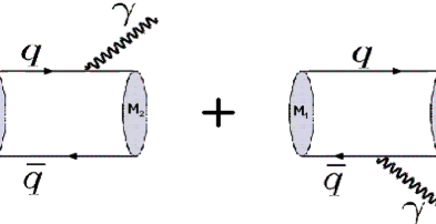
2 Impulse approximation

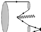
The impulse approximation is widely used in studies of meson transitions and form-factors. In this approximation the possibility of quark-antiquark pair creation from the vacuum is neglected. The interaction of the external current with the meson is the sum of its coupling to quark and antiquark as illustrated in figure 2. In the diagrams, $M_{1}$ and $M_{2}$ are the initial and final state mesons (bound states of quark $q$ and antiquark $\bar{q}$, which are represented by lines with arrows). In this section, our approach to the calculations of the form-factors and radiative transition decay rates in the impulse approximation of the quark model is presented.

Figure 2: Impulse approximation diagrams.

Form factors are a powerful determinant of internal hadronic structure because the external current momentum serves as a probe scale. And of course, different currents are sensitive to different properties of the hadron, so it is useful to study the form-factors when tuning and testing models.

The technique used to compute the form factors is illustrated by considering the inelastic pseudoscalar electromagnetic matrix element $\langle P_{2}|J^{\mu}|P_{1}\rangle$, where $P$ refers to a pseudoscalar meson. The most general Lorentz covariant decomposition of this matrix element is

$$\langle P_{2}(p_{2})|\bar{\Psi}(0)\gamma^{\mu}\Psi(0)|P_{1}(p_{1})\rangle=f(Q^{2})\left((p_{2}+p_{1})^{\mu}-\frac{M^{2}_{2}-M^{2}_{1}}{q^{2}}(p_{2}-p_{1})^{\mu}\right)$$ (54)

where conservation of the vector current has been used to eliminate a possible second invariant. The argument of the form factor is chosen to be $Q^{2}=-(p_{2}-p_{1})_{\mu}(p_{2}-p_{1})^{\mu}$.

Now the matrix element on the left could be calculated in some model, for example in the quark model, and then the result for the form-factor $f(Q^{2})$ could be compared to the experimental data (if available).

In the impulse approximation, using the temporal component of the vector current and computing in the rest frame of the initial meson yields

$$f_{sq}(Q^{2}) = \frac{\sqrt{M_{1}E_{2}}}{(E_{2}+M_{1})-\frac{M^{2}_{2}-M^{2}_{1}}{q^{2}}(E_{2}-M_{1})}$$

$$\times \int\frac{d^{3}k}{(2\pi)^{3}}\Phi(\vec{k})\Phi^{*}\left(\vec{k}+\vec{q}\frac{\bar{m}_{2}}{m_{2}+\bar{m}_{2}}\right)\sqrt{1+\frac{m_{1}}{E_{k}}}\sqrt{1+\frac{m_{2}}{E_{k+q}}}\left(1+\frac{(\vec{k}+\vec{q})\cdot\vec{k}}{(E_{k}+m_{1})(E_{k+q}+m_{2})}\right).$$

The pseudoscalars are assumed to have valence quark masses $m_{1},\bar{m}_{1}$ and $m_{2},\bar{m}_{2}$ for $P_{1}$ and $P_{2}$ respectively. The masses of the mesons are labeled $M_{1}$ and $M_{2}$. The single quark elastic form factor can be obtained by setting $m_{1}=\bar{m}_{1}=m_{2}=\bar{m}_{2}$ and $M_{1}=M_{2}$. In the nonrelativistic limit Eq. 2 reduces to the simple expression:

$$f_{sq}(Q^{2})=\int\frac{d^{3}k}{(2\pi)^{3}}\Phi(\vec{k})\Phi^{*}\left(\vec{k}+\frac{\vec{q}}{2}\right).$$ (56)

In this case it is easy to see the normalization condition $f_{sq}(\vec{q}=0)=1$. This is also true for the relativistic elastic single quark form factor of Eq. 2.

To calculate the decay rate of the radiative transition $M_{1}\rightarrow\gamma M_{2}$ we need to know the electromagnetic matrix element $\langle M_{2}|J^{\mu}|M_{1}\rangle$ at $q^{2}=0$, where $M_{1}$ and $M_{2}$ are the initial and final meson states. In the impulse approximation using the vector component of the current we have:

$$\vec{A}_{em} \equiv \langle M_{2}|\vec{J}|M_{1}\rangle=eQ_{q}\langle M_{2}|\vec{J}^{(q)}|M_{1}\rangle+eQ_{\bar{q}}\langle M_{2}|\vec{J}^{(\bar{q})}|M_{1}\rangle,$$ (57)

$$\vec{J}^{(q)} = -u^{\dagger}_{s_{2}}({k_{2}})\,{\vec{\alpha}}\,u_{s_{1}}(k_{1}),$$

$$\vec{J}^{(\bar{q})} = -v^{\dagger}_{\bar{s}_{1}}(\bar{k}_{1})\,{\vec{\alpha}}\,v_{\bar{s}_{2}}(\bar{k}_{2}).$$

where ${\bf{k}}_{1},\bar{\bf{k}}_{1},s_{1}$ and $\bar{s}_{1}$ are the momenta and spins of the quark and antiquark of the initial state meson, and $\bf{k}_{2},\bar{\bf{k}}_{2},s_{2},\bar{s}_{2}$ are the corresponding momenta and spins of the final state meson. $Q_{q}$ and $Q_{\bar{q}}$ are the quark and antiquark charges. The two terms of (57) corresponds to the quark and antiquark electromagnetic interactions.

It is very common to consider quark and antiquark being nonrelativistic when studying radiative transition. We investigate the validity of this approximation by comparing two cases: taking the full relativistic expressions for quark and antiquark spinors and then comparing our results to those calculated with the nonrelativistic approximation. We find considerable differences for the decay rates, even for heavy mesons, as will be shown in Chapter 6, and conclude that quarks should be treated relativistically.

We illustrate the technique used to study radiative transitions for the nonrelativistic approximation of the quark spinors. The treatment of the case with full relativistic expressions for spinors is completely analogous, except for much more complicated expressions for the matrix elements. The study of full relativistic case have been performed numerically.

In the rest frame of the initial state meson we have:

$$\vec{A}_{em}=\frac{eQ_{q}}{2m_{q}}\,\Big{\langle}M_{2}\Big{|}(2\vec{k}+\vec{q})\delta_{s_{1}s_{2}}-i\vec{q}\times\vec{\sigma}_{21}\Big{|}M_{1}\Big{\rangle}+\frac{eQ_{\bar{q}}}{2m_{\bar{q}}}\,\Big{\langle}M_{2}\Big{|}(2\vec{k}-\vec{q})\delta_{\bar{s}_{1}\bar{s}_{2}}-i\vec{q}\times\vec{\sigma}_{\bar{1}\bar{2}}\Big{|}M_{1}\Big{\rangle},$$ (58)

where $\vec{\sigma}_{21}=\chi^{{\dagger}}_{s_{2}}\vec{\sigma}\chi_{s_{1}}$ and $\vec{\sigma}_{\bar{1}\bar{2}}=\tilde{\chi}^{{\dagger}}_{\bar{s}_{1}}\vec{\sigma}\tilde{\chi}_{\bar{s}_{2}}$, here $\chi_{s}$ is the Dirac spinor for quark or antiquark.

Radiative transitions are usually said to be either of electric or magnetic type depending on the dominating term in multipole expansion of the amplitude. If the initial and final state mesons have different spins but same angular momentum then the transition is magnetic, and the contribution of the terms proportional to $\delta_{s_{1}s_{2}}$ or $\delta_{\bar{s}_{1}\bar{s}_{2}}$ in expression 58 is zero. The example of the magnetic transition is the vector to pseudoscalar meson transition ${}^{3}S_{1}\rightarrow\,^{1}S_{0}\,\gamma$.

If the initial and final states have different angular momentum then the transition is electric and all the terms in 58 contribute to the amplitude. An example of the electric transition is P-wave state to the vector meson state transition ${}^{3}P_{0}\rightarrow\,^{3}S_{1}\gamma$.

Very often when considering electric transitions the second term in the square brackets of (58) is ignored, which is called the dipole approximation, and also the limit $\vec{q}\rightarrow 0$ is taken, which corresponds to the long-wavelength approximation. In this case the expression for the amplitude of E1 transitions is very simple:

$$\vec{A}_{em}=\langle M_{2}|\vec{k}|M_{1}\rangle\left[\frac{eQ_{q}}{m_{q}}+\frac{eQ_{\bar{q}}}{m_{\bar{q}}}\right]\delta_{s_{1}s_{2}}\delta_{\bar{s}_{1}\bar{s}_{2}}$$ (59)

Using Siegert’s theorem one can write $i[H,r]=2p/m_{q}$ and then the transition amplitude is proportional to the matrix element $\langle M_{2}|r|M_{1}\rangle$.

The technique described in the previous paragraph is the usual way to calculate radiative transitions in the literature. We have tested the validity of the approximations typically made. In particular, we have taken into account all terms in the operator of the equation (58) and we have not made the zero recoil approximation. Comparing the results of our calculations to the results with usual approximations in Chapter 6 we find significant differences and conclude that it is important to treat radiative transitions carefully in the most possible general way.

Matrix elements in (58) could be calculated using the quark model meson state (1). For example, for vector meson to pseudoscalar meson transition $V\rightarrow P\gamma$ in the nonrelativistic approximation for the quark spinors it is:

$$\vec{A}_{em}(\!\!\!\! V \!\rightarrow P\gamma)=-2i\left(\vec{q}\times\vec{\epsilon}_{V}\right)\sqrt{M_{1}E_{2}}\times$$

$$\times \left[\frac{eQ_{q}}{2m_{q}}\int\frac{d^{3}\vec{k}}{(2\pi)^{3}}\Phi^{*}_{2}\left({\vec{k}}+\frac{m_{\bar{q}}}{m_{q}+m_{\bar{q}}}\vec{q}\right)\Phi_{1}(\vec{k})+\frac{eQ_{\bar{q}}}{2m_{\bar{q}}}\int\frac{d^{3}\vec{k}}{(2\pi)^{3}}\Phi^{*}_{2}\left(\vec{k}-\frac{m_{q}}{m_{q}+m_{\bar{q}}}\vec{q}\right)\Phi_{1}(\vec{k})\right],$$

where $\vec{\epsilon}_{V}$ is the polarization vector of the vector meson, $\Phi(k)_{(1,2)}$ are the spatial wave function of initial and final state mesons in the momentum space, $M_{1}$ is the mass of the initial state meson and $E_{2}$ is the energy of the final state meson.

As an approximation to the meson wave function, spherical harmonic oscillator wave functions are widely in use. This approximation greatly simplifies the calculations, and most of the quantities of interest could be calculated analytically. Thus we conclude that it is reasonably good for the crude estimation of the ground state meson wave function and main features of matrix elements but for qualitative studies realistic meson wave functions should be employed. Another use of this approximation is testing the numerical methods which then could be applied to the more complex cases.

The SHO spatial wave function for vector and pseudoscalar mesons is:

$$\Phi(k)=\left(\frac{4\pi}{\beta^{2}}\right)^{3/4}e^{-k^{2}/2\beta^{2}},$$ (61)

and then the amplitude (2) for $V\rightarrow P\gamma$ in the SHO nonrelativistic approximation is:

$$\vec{A}_{em}=-2i\left(\vec{q}\times\vec{\epsilon}_{V}\right)\sqrt{M_{1}E_{2}}\left[\frac{eQ_{q}}{2m_{q}}e^{-{\mu^{2}q^{2}}/4\beta^{2}}+\frac{eQ_{\bar{q}}}{2m_{\bar{q}}}e^{-{\bar{\mu}^{2}q^{2}}/4\beta^{2}}\right],$$ (62)

where

$$\mu=\frac{m_{\bar{q}}}{m_{q}+m_{\bar{q}}}\,\,\,\,\,\,\,\,\,and\,\,\,\,\,\,\,\,\,\bar{\mu}=\frac{m_{q}}{m_{q}+m_{\bar{q}}}.$$ (63)

In the special case of $m_{q}=m_{\bar{q}}$ we have $\mu=\bar{\mu}=1/2$ and:

$$\vec{A}_{em}=-i\left(\vec{q}\times\vec{\epsilon}_{V}\right)\sqrt{M_{1}E_{2}}\frac{eQ_{q}+eQ_{\bar{q}}}{m_{q}}e^{-{q^{2}}/16\beta^{2}}.$$ (64)

The decay rate for a radiative transition is:

$$\Gamma(M_{2}\rightarrow M_{1}\gamma)=\frac{1}{32\pi^{2}}\frac{1}{2J_{1}+1}\int d\Omega_{\hat{q}}\frac{|\vec{q}|}{M^{2}_{1}}\sum_{\lambda,V}|\vec{\epsilon}^{\,*}_{\lambda}\cdot\vec{A}_{em}|^{2}.$$ (65)

In our example for $V\rightarrow P\gamma$ using SHO wave functions the decay rate is:

$$\Gamma(V\rightarrow P\gamma)=\frac{\alpha}{3}\frac{E_{2}|\vec{q}|^{3}}{M_{1}}\left[\frac{Q_{q}}{m_{q}}e^{-{\mu^{2}q^{2}}/4\beta^{2}}+\frac{Q_{\bar{q}}}{m_{\bar{q}}}e^{-{\bar{\mu}^{2}q^{2}}/4\beta^{2}}\right]^{2},$$ (66)

The same approach could be used for any other meson radiative transitions. The results of our calculations for a variety of models, discussion of the effects of approximations described above and comparison to the experiment are presented in Chapter 6.

3 Higher order diagrams

Higher order diagrams take into account the possibility of quark-antiquark pair appearing from the vacuum. Studying these diagrams is important as they might give significant contribution to the impulse approximation since there is no small parameter associated with the quark-antiquark pair creation in low energy QCD.

Figure 3: Higher order diagrams in Cornell model.

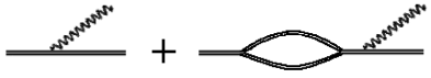
One way to introduce higher order diagrams was developed by Cornell group [65], the so called ‘Cornell’ model. In this model the mesonic state is described as a superposition of a naive quark-antiquark state and all possible decay channels of a naive state into two other mesons. There are two diagrams contributing to the radiative transition, shown in Fig. 3. Mesons in the Cornell model diagrams are represented by double line. The first diagram corresponds to the impulse approximation and the second diagram is higher order. However, for this model to be consistent, coupling of the electromagnetic current to the products of the decay in the intermediate state should also be taken into account, for example, diagram shown in Fig. 4 should be considered. These kinds of diagrams have been neglected in [65].

Figure 4: Higher order diagram not taken into account in Cornell model.

Figure 5: Higher order diagrams in the bound state time ordered perturbation theory.

We offer a different way of describing higher order diagrams in radiative transitions. In our approach, we use ${}^{3}P_{0}$ model to describe the quark-antiquark pair creation (${}^{3}P_{0}$ model is explained in section 2) and then employ the bound state time ordered perturbation theory to obtain higher order diagrams. There are two diagrams which contribute to the transition in addition to the impulse approximation, they are shown in Fig. 5. When calculating the diagrams in the quark model all possible intermediate bound states have to be summed over. Details of the calculations and our estimations of these diagrams are presented in Chapter 6.

4 Gamma-gamma transitions

Two-photon decays of mesons are of considerable interest as a search mode, a probe of internal structure, and as a test of nonperturbative QCD modeling. An illustration of the importance of the latter point is the recent realization that the usual factorization approach to orthopositronium (and its extensions to QCD) decay violates low energy theorems[66].

It has been traditional to compute decays such as $Ps\to\gamma\gamma$ by assuming factorization between soft bound state dynamics and hard rescattering into photons[67]. This approximation is valid when the photon energy is much greater than the binding energy $E_{B}\sim m\alpha^{2}$. This is a difficult condition to satisfy in the case of QCD where $\alpha\to\alpha_{s}\sim 1$. Nevertheless, this approach has been adopted to inclusive strong decays of mesons[68, 69, 70] and has been extensively applied to two-photon decays of quarkonia[71].

The application of naive factorization to orthopositronium decay (or $M\to ggg$, $\gamma gg$ in QCD) leads to a differential decay rate that scales as $E_{\gamma}$ for small photon energies[72] – at odds with the $E_{\gamma}^{3}$ behavior required by gauge invariance and analyticity (this is Low’s theorem[73]). The contradiction can be traced to the scale dependence of the choice of relevant states and can be resolved with a careful NRQED analysis[74]. For example, a parapositronium-photon intermediate state can be important in orthopositronium decay at low energy. Other attempts to address the problem by treating the binding energy nonperturbatively can be found in Refs. [75, 76].

Naive factorization is equivalent to making a vertical cut through the loop diagram representing $Ps\to n\gamma$[75] (see Fig. 6). Of course this ignores cuts across photon vertices that correspond to the neglected intermediate states mentioned above. In view of this, a possible improvement is to assume that pseudoscalar meson decay to two photons occurs via an intermediate vector meson followed by a vector meson dominance transition to a photon. This approach was indeed suggested long ago by van Royen and Weisskopf[64] who made simple estimates of the rates for $\pi^{0}\to\gamma\gamma$ and $\eta\to\gamma\gamma$. This proposal is also in accord with time ordered perturbation theory applied to QCD in Coulomb gauge, where intermediate bound states created by instantaneous gluon exchange must be summed over.

Figure 6: Naive Factorization in Positronium Decay.

Finally, one expects that an effective description should work for sufficiently low momentum photons. The effective Lagrangian for pseudoscalar decay can be written as

$${\cal L}=g\int\eta F^{\mu\nu}\tilde{F}_{\mu\nu}$$ (67)

leading to the prediction $\Gamma(\eta\to\gamma\gamma)\propto g^{2}m_{\eta}^{3}$. Since this scaling with respect to the pseudoscalar mass appears to be experimentally satisfied for $\pi$, $\eta$, $\eta^{\prime}$ mesons, Isgur et al. inserted an ad hoc dependence of $m_{\eta}^{3}$ in their quark model computations[63, 77]. While perhaps of practical use, this approach is not theoretically justified and calls into doubt the utility of the quark model in this context. Indeed simple quark model computations of the amplitude of Fig. 6 are not dependent on binding energies and can only depend on kinematic quantities such as quark masses.

In view of the discussion above, we chose to abandon the factorization approach and compute two-photon charmonium decays in the quark model in bound state time ordered perturbation theory. This has the effect of saturating the intermediate state with all possible vectors, thereby bringing in binding energies, a nontrivial dependence on the pseudoscalar mass, and incorporating oblique cuts in the loop diagram.

Details of our calculations and the results are presented in Chapter 5.

5 Meson transitions in ‘Coulomb gauge model’

As was described in section 2, a relativistic many-body approach in Coulomb gauge (‘Coulomb gauge model’) is a richer model of hadron structure than the nonrelativistic potential model. It can explain some fundamental properties of QCD, such as chiral symmetry breaking and dependence of the quark mass on the energy scale, in a fully relativistic way. Until now only meson spectra have been calculated in this model, and the agreement with the experiment is impressive. However, for testing and improving the model, other meson properties should be investigated.

For Coulomb gauge model the same approach to the calculation of the meson properties could be used as for the nonrelativistic potential quark model, the main difference being the spatial meson wave functions. As was explained in section 2 in order to calculate spatial meson wave function in RPA approximation we need to solve the system of two nonlinear coupled integral equations. After that the formulas from appendices 8 and 9 could be used to calculate form-factors, decay constants and radiative transitions.

The only practical exception of the statement above is the study of pion properties. In RPA approximation the wave function of each meson is a superposition of the forward and backward propagating components. The backward propagating component is negligible for all the mesons, except pion. In the pion case this leads to a change in the wave function normalization and has a considerable effect on the pion properties. As an example, our results for radiative transition decay rates involving pion will be presented in Chapter 6. They have much better agreement with the experiment in Coulomb gauge model than in the nonrelativistic potential model.

Chapter 2 SPECTROSCOPY

New spectroscopy from the B factories and the advent of CLEO-c and the BES upgrade have led to a resurgence of interest in charmonia. Among the new developments are the discovery of the $\eta_{c}^{\prime}$ and $h_{c}$ mesons and the observation of the enigmatic $X(3872)$ and $Y(4260)$ states at Belle[78].

BaBar’s discovery of the $D_{s}(2317)$ state[79] generated strong interest in heavy meson spectroscopy – chiefly due to its surprisingly low mass with respect to expectations. These expectations are based on quark models or lattice gauge theory. Unfortunately, at present large lattice systematic errors do not allow a determination of the $D_{s}$ mass with a precision better than several hundred MeV. And, although quark models appear to be exceptionally accurate in describing charmonia, they are less constrained by experiment and on a weaker theoretical footing in the open charm sector. It is therefore imperative to examine reasonable alternative descriptions of the open charm sector.

The $D_{s}(2317)$ was produced in $e^{+}e^{-}$ scattering and discovered in the isospin violating $D_{s}\pi$ decay mode in $K\bar{K}\pi\pi$ and $K\bar{K}\pi\pi\pi$ mass distributions. Its width is less than 10 MeV and it is likely that the quantum numbers are $J^{P}=0^{+}$[78]. Finally, if the $D_{s}\pi^{0}$ mode dominates the width of the $D_{s}(2317)$ then the measured product of branching ratios[80]

$$Br(B^{0}\to D_{s}(2317)K)\cdot Br(D_{s}(2317)\to D_{s}\pi^{0})=(4.4\pm 0.8\pm 1.1)\cdot 10^{-5}$$ (1)

implies that $Br(B\to D_{s}(2317)K)\approx Br(B\to D_{s}K)$, consistent with the $D_{s}(2317)$ being a canonical $0^{+}$ $c\bar{s}$ meson.

In view of this, Cahn and Jackson have examined the feasibility of describing the masses and decay widths of the low lying $D$ and $D_{s}$ states within the constituent quark model[35]. They assume a standard spin-dependent structure for the quark-antiquark interaction (see below) and allow general vector and scalar potentials. Their conclusion is that it is very difficult to describe the data in this scenario.

Indeed, the $D_{s}(2317)$ lies some 160 MeV below most model predictions (see Ref.[78] for a summary), leading to speculation that the state could be a $DK$ molecule[81] or a tetraquark[82]. Such speculation is supported by the isospin violating discovery mode of the $D_{s}(2317)$ and the proximity of the S-wave $DK$ threshold at 2358-2367 MeV.

Although these proposals have several attractive features, it is important to exhaust possible canonical $c\bar{s}$ descriptions of the $D_{s}(2317)$ before resorting to more exotic models. In section 3 we propose a simple modification to the standard vector Coulomb+scalar linear quark potential model that maintains good agreement with the charmonium spectrum and agrees remarkably well with the $D$ and $D_{s}$ spectra. Possible experimental tests of this scenario are discussed.

Below the results of our study of charmonium, bottomonium and open charm spectroscopy are presented and discussed.

1 Charmonium

We adopt the standard practice of describing charmonia with nonrelativistic kinematics, a central confining potential, and order $v^{2}/c^{2}$ spin-dependent interactions. Thus $H=2m+P_{rel}^{2}/2\mu+V_{C}+V_{SD}$ where

$$V_{C}(r)=-\frac{4}{3}\frac{\alpha_{C}}{r}+br,$$ (2)

and

$$V_{SD}(r)=\frac{32\alpha_{H}\pi e^{-k^{2}/4\sigma^{2}}}{9m_{q}^{2}}\vec{S}_{q}\cdot\vec{S}_{\bar{q}}+\Big{(}\frac{2\alpha_{s}}{r^{3}}-\frac{b}{2r}\Big{)}\frac{1}{m_{q}^{2}}\vec{L}\cdot\vec{S}+\frac{4\alpha_{s}}{m_{q}^{2}r^{3}}T,$$ (3)

where $3T=3\hat{r}\cdot S_{q}\hat{r}\cdot\vec{S}_{\bar{q}}-\vec{S}_{q}\cdot\vec{S}_{\bar{q}}$. The strengths of the Coulomb and hyperfine interactions have been taken as separate parameters. Perturbative gluon exchange implies that $\alpha_{C}=\alpha_{H}$ and we find that the fits prefer the near equality of these parameters. The variation of this model, as described in section 1, includes running coupling 5.

The resulting low lying spectra are presented in Table 9. The first column presents the results of the ‘BGS’ model[31], which was tuned to the available charmonium spectrum. Parameters are: $m_{c}=1.4794$ GeV, $\alpha_{c}=\alpha_{H}=0.5461$, $\sigma=1.0946$ GeV, and $b=0.1425$ GeV². No constant is included.

The second and third columns, labeled BGS+log, makes the replacement of Eq. 5; the parameters have not been retuned. One sees that the $J/\psi$ and $\eta_{c}$ masses have been raised somewhat and that the splitting has been reduced to 80 MeV. Heavier states have only been slightly shifted. It is possible to fit the $J/\psi$ and $\eta_{c}$ masses by adjusting parameters, however this tends to ruin the agreement of the model with the excited states. We therefore choose to compare the BGS and BGS+log models without any further adjustment to the parameters. A comparison with other models and lattice gauge theory can be found in Ref. [78].

Table 1: Spectrum of $c\bar{c}$ mesons (GeV).

state	BGS	BGS log	BGS log	experiment
		$\Lambda=0.25$ GeV	$\Lambda=0.4$ GeV
$\eta_{c}(1^{1}S_{0})$	2.981	3.088	3.052	2.979
$\eta_{c}(2^{1}S_{0})$	3.625	3.669	3.655	3.638
$\eta_{c}(3^{1}S_{0})$	4.032	4.067	4.057	-
$\eta_{c}(4^{1}S_{0})$	4.364	4.398	4.391	-
$\eta_{c2}(1^{1}D_{2})$	3.799	3.803	3.800	-
$\eta_{c2}(2^{1}D_{2})$	4.155	4.158	4.156	-
$J/\psi(1^{3}S_{1})$	3.089	3.168	3.139	3.097
$\psi(2^{3}S_{1})$	3.666	3.707	3.694	3.686
$\psi(3^{3}S_{1})$	4.060	4.094	4.085	4.040
$\psi(4^{3}S_{1})$	4.386	4.420	4.412	4.415
$\psi(1^{3}D_{1})$	3.785	3.789	3.786	3.770
$\psi(2^{3}D_{1})$	4.139	4.143	4.141	4.159
$\psi_{2}(1^{3}D_{2})$	3.800	3.804	3.801	-
$\psi_{2}(2^{3}D_{2})$	4.156	4.159	4.157	-
$\psi_{3}(1^{3}D_{3})$	3.806	3.809	3.807	-
$\psi_{3}(2^{3}D_{3})$	4.164	4.167	4.165	-
$\chi_{c0}(1^{3}P_{0})$	3.425	3.448	3.435	3.415
$\chi_{c0}(2^{3}P_{0})$	3.851	3.870	3.861	-
$\chi_{c0}(3^{3}P_{0})$	4.197	4.214	4.207	-
$\chi_{c1}(1^{3}P_{1})$	3.505	3.520	3.511	3.511
$\chi_{c1}(2^{3}P_{1})$	3.923	3.934	3.928	-
$\chi_{c1}(3^{3}P_{1})$	4.265	4.275	4.270	-
$\chi_{c2}(1^{3}P_{2})$	3.556	3.564	3.558	3.556
$\chi_{c2}(2^{3}P_{2})$	3.970	3.976	3.972	-
$\chi_{c2}(3^{3}P_{2})$	4.311	4.316	4.313	-
$h_{c}(1^{1}P_{1})$	3.524	3.536	3.529	-
$h_{c}(2^{1}P_{1})$	3.941	3.950	3.945	-
$h_{c}(3^{1}P_{1})$	4.283	4.291	4.287	-

Meson spectrum is not a particularly robust test of model reliability because it only probes gross features of the wavefunction. Alternatively, observables such as strong and electroweak decays and production processes probe different wavefunction momentum scales. For example, decay constants are short distance observables while strong and radiative transitions test intermediate scales. Thus the latter do not add much new information unless the transition occurs far from the zero recoil point. In this case the properties of boosted wavefunctions and higher momentum components become important. Production processes can provide information on the short distance behavior of the wavefunctions since much experimental data is available. Unfortunately, the underlying mechanisms at work are still under debate, even for $J/\psi$ and $\psi^{\prime}$ [83].

2 Bottomonium

The bottomonium parameters were obtained by fitting the potential model of Eqs. 4 and 3 (C+L) to the known bottomonium spectrum. The results are $m_{b}=4.75$ GeV, $\alpha_{C}=\alpha_{H}=0.35$, $b=0.19$ GeV², and $\sigma=0.897$ GeV. All the calculations have been performed as for charmonia.

Table 2: Bottomonium Spectrum (GeV).

Meson	C+L	C+L log	C+L log	PDG
		$\Lambda=0.4$ GeV	$\Lambda=0.25$ GeV
$\eta_{b}$	9.448	9.490	9.516
$\eta_{b}^{\prime}$	10.006	10.023	10.033
$\eta_{b}^{\prime\prime}$	10.352	10.365	10.372
$\Upsilon$	9.459	9.500	9.525	$9.4603\pm 0.00026$
$\Upsilon^{\prime}$	10.009	10.026	10.036	$10.02326\pm 0.00031$
$\Upsilon^{\prime\prime}$	10.354	10.367	10.374	$10.3552\pm 0.0005$
$\chi_{b0}$	9.871	9.873	9.879	$9.8599\pm 0.001$
$\chi_{b0}^{\prime}$	10.232	10.235	10.239	$10.2321\pm 0.0006$
$\chi_{b0}^{\prime\prime}$	10.522	10.525	10.529
$\chi_{b1}$	9.897	9.900	9.904	$9.8927\pm 0.0006$
$\chi_{b1}^{\prime}$	10.255	10.257	10.260	$10.2552\pm 0.0005$
$\chi_{b1}^{\prime\prime}$	10.544	10.546	10.548
$\chi_{b2}$	9.916	9.917	9.921	$9.9126\pm 0.0005$
$\chi_{b2}^{\prime}$	10.271	10.272	10.275	$10.2685\pm 0.0004$
$\chi_{b2}^{\prime\prime}$	10.559	10.560	10.563

Second and third columns correspond to the model with logarithmic dependence of running coupling 5. The parameters of the potential have not been refitted. One can see that, as for charmonium, introducing the running coupling has a small effect on the excited states while considerably shifting ground state masses of $\eta_{b}$ and $\Upsilon$.

3 Spectroscopy of Open Charm States

The spectra we seek to explain are summarized in Table 3. Unfortunately, the masses of the $D_{0}$ (labeled $a$) and $D_{1}^{\prime}$ (labeled $b$) are poorly determined. Belle have observed[84] the $D_{0}$ in $B$ decays, and claim a mass of $2308\pm 17\pm 32$ MeV with a width of $\Gamma=276\pm 21\pm 18\pm 60$ MeV, while FOCUS[85] find $2407\pm 21\pm 35$ MeV with a width $\Gamma=240\pm 55\pm 59$ MeV. While some authors choose to average these values, we regard them as incompatible and consider the cases separately below. Finally, there is an older mass determination from Belle[86] of $2290\pm 22\pm 20$ MeV with a width of $\Gamma=305\pm 30\pm 25$. The $D_{1}^{\prime}$ has been seen in $B$ decays to $D\pi\pi$ and $D^{*}\pi\pi$ by Belle [84]. A Breit-Wigner fit yields a mass of $2427\pm 26\pm 20\pm 15$ MeV and a width of $384^{+107}_{-90}\pm 24\pm 70$ MeV. Alternatively, a preliminary report from CLEO[87] cites a mass of $2461^{+41}_{-34}\pm 10\pm 32$ MeV and a width of $290^{+101}_{-79}\pm 26\pm 36$ MeV. Finally, FOCUS [88] obtain a lower neutral $D_{1}^{\prime}$ mass of $2407\pm 21\pm 35$ MeV. Other masses in Table 3 are obtained from the PDG compilation[89].

Table 3: Low Lying $D$ and $D_{s}$ Spectra

$J^{P}$	$0^{-}$	$1^{-}$	$0^{+}$	$1^{+}$	$1^{+}$	$2^{+}$
$D$	$1869.3\pm 0.5$	$2010.0\pm 0.5$	a	b	$2422.2\pm 1.8$	$2459\pm 4$
$D_{s}$	$1968.5\pm 0.6$	$2112.4\pm 0.7$	$2317.4\pm 0.9$	$2459.3\pm 1.3$	$2535.35\pm 0.34$	$2572.4\pm 1.5$

In addition to the unexpectedly low mass of the $D_{s}(2317)$, the $D_{s}(2460)$ is also somewhat below predictions (Godfrey and Isgur, for example, predict a mass of 2530 MeV[77]). It is possible that an analogous situation holds in the $D$ spectrum, depending on the mass of the $D_{0}$. The quark model explanation of these states rests on P-wave mass splittings induced by spin-dependent interactions.

Here we propose to take the spin-dependence of Eq. 8 seriously and examine its effect on low-lying heavy-light mesons. Our model can be described in terms of vector and scalar kernels defined by

$$V_{conf}=V+S$$ (4)

where $V=-4\alpha_{s}/3r$ is the vector kernel and $S=br$ is the scalar kernel, and by the order $\alpha_{s}^{2}$ contributions to the $V_{i}$, denoted by $\delta V_{i}$. Expressions for the matrix elements of the spin-dependent interaction are then

$$V_{1} = -S+\delta V_{1}$$ (5)

$$V_{2} = V+\delta V_{2}$$ (6)

$$V_{3} = V^{\prime}/r-V^{\prime\prime}+\delta V_{3}$$ (7)

$$V_{4} = 2\nabla^{2}V+\delta V_{4}$$ (8)

$$V_{5} = \delta V_{5}$$ (9)

Explicitly,

$$V_{1}(m_{q},m_{\bar{q}},r) = -br-C_{F}\frac{1}{2r}\frac{\alpha_{s}^{2}}{\pi}\left(C_{F}-C_{A}\left(\ln{\left[(m_{q}m_{\bar{q}})^{1/2}r\right]}+\gamma_{E}\right)\right)$$

$$V_{2}(m_{q},m_{\bar{q}},r) = -\frac{1}{r}C_{F}\alpha_{s}\left[1+\frac{\alpha_{s}}{\pi}\left[\frac{b_{0}}{2}[\ln{(\mu r)}+\gamma_{E}]+\frac{5}{12}b_{0}-\frac{2}{3}C_{A}+\right.\right.$$

$$+\left.\left.\frac{1}{2}\left(C_{F}-C_{A}\left(\ln{\left[(m_{q}m_{\bar{q}})^{1/2}r\right]}+\gamma_{E}\right)\right)\right]\right]$$

$$V_{3}(m_{q},m_{\bar{q}},r) = \frac{1}{r^{3}}3C_{F}\alpha_{s}\left[1+\frac{\alpha_{s}}{\pi}\left[\frac{b_{0}}{2}[\ln{(\mu r)}+\gamma_{E}-\frac{4}{3}]+\frac{5}{12}b_{0}-\frac{2}{3}C_{A}+\right.\right.$$

$$+\left.\left.\frac{1}{2}\left(C_{A}+2C_{F}-2C_{A}\left(\ln{\left[(m_{q}m_{\bar{q}})^{1/2}r\right]}+\gamma_{E}-\frac{4}{3}\right)\right)\right]\right]$$

$$V_{4}(m_{q},m_{\bar{q}},r) = \frac{32\alpha_{s}\sigma^{3}e^{-\sigma^{2}r^{2}}}{3\sqrt{\pi}}$$

$$V_{5}(m_{q},m_{\bar{q}},r) = \frac{1}{4r^{3}}C_{F}C_{A}\frac{\alpha_{s}^{2}}{\pi}\ln{\frac{m_{\bar{q}}}{m_{q}}}$$ (10)

where $C_{F}=4/3$, $C_{A}=3$, $b_{0}=9$, $\gamma_{E}=0.5772$, the scale $\mu$ has been set to 1 GeV.

The hyperfine interaction (proportional to $V_{4}$) contains a delta function in configuration space and is normally ‘smeared’ to make it nonperturbatively tractable. For this reason we choose not to include $\delta V_{4}$ in the model definition of Eq. 10. In following, the hyperfine interaction ($V_{4}$) have been included in the meson wave function calculations and the remaining spin-dependent terms are treated as mass shifts using leading-order perturbation theory.

We have confirmed that the additional features do not ruin previous agreement with, for example, the charmonium spectrum. For example, Ref. [31] obtains very good agreement with experiment for parameters $m_{c}=1.4794$ GeV, $\alpha_{s}=0.5461$, $b=0.1425$ GeV², and $\sigma=1.0946$ GeV. Employing the model of Eqn. 10 worsens the agreement with experiment, but the original good fit is recovered upon slightly modifying parameters (the refit parameters are $m_{c}=1.57$ GeV, $\alpha_{s}=0.52$, $b=0.15$ GeV², and $\sigma=1.3$ GeV).

Table 4: Model Parameters

model	$\alpha_{s}$	$b$ (GeV2)	$\sigma$ (GeV)	$m_{c}$ (GeV)	$C$ (GeV)
low	0.46	0.145	1.20	1.40	-0.298
avg	0.50	0.140	1.17	1.43	-0.275
high	0.53	0.135	1.13	1.45	-0.254

The low lying $c\bar{s}$ and $c\bar{u}$ states are fit reasonably well with the parameters labeled ‘avg’ in Table 4. Predicted masses are given in Table 5. Parameters labeled ‘low’ in Table 4 fit the $D$ mesons very well, whereas those labeled ‘high’ fit the known $D_{s}$ mesons well. It is thus reassuring that these parameter sets are reasonably similar to each other and to the refit charmonium parameters. (Note that constant shifts in each flavor sector are fit to the relevant pseudoscalar masses.)

The predicted $D_{s0}$ mass is 2341 MeV, 140 MeV lower than the prediction of Godfrey and Isgur and only 24 MeV higher than experiment. We remark that the best fit to the $D$ spectrum predicts a mass of 2287 MeV for the $D_{0}$ meson, in good agreement with the preliminary Belle measurement of 2290 MeV, 21 MeV below the current Belle mass, and in disagreement with the FOCUS mass of 2407 MeV.

The average error in the predicted P-wave masses is less than 1%. It thus appears likely that the simple modification to the spin-dependent quark interaction is capable of describing heavy-light mesons with reasonable accuracy.

Table 5: Low Lying Charm Meson Spectra (GeV)

flavor	$0^{-}$	$1^{-}$	$0^{+}$	$1^{+}$	$1^{+}$	$2^{+}$
$D$	1.869	2.017	2.260	2.406	2.445	2.493
$D_{s}$	1.968	2.105	2.341	2.475	2.514	2.563

We examine the new model in more detail by computing P-wave meson masses (with respect to the ground state vector) as a function of the heavy quark mass. Results for $Q\bar{u}$ and $Q\bar{s}$ systems are displayed in Fig. 1. One sees a very slow approach to the expected heavy quark doublet structure. Level ordering ($D_{2}>D_{1}^{\prime},D_{1}>D_{0}$) is maintained for all heavy quark masses. This is not the case in the canonical quark model, and ruins the agreement with experiment at scales near the charm quark mass. It is intriguing that the scalar-vector mass difference gets very small for light $Q$ masses, raising the possibility that the enigmatic $a_{0}$ and $f_{0}$ mesons may simply be $q\bar{q}$ states.

Finally, one obtains $M(h_{c})>M(\chi_{c1})$ in one-loop and traditional models, in agreement with experiment. However, experimentally $M(f_{1})-M(h_{1})\approx 100$ MeV and $M(a_{1})-M(b_{1})\approx 0$ MeV, indicating that the ${}^{3}P_{1}$ state is heavier than (or nearly degenerate with) the ${}^{1}P_{1}$ light meson state. Thus the sign of the combination of tensor and spin-orbit terms that drives this splitting must change when going from charm quark to light quark masses. This change is approximately correctly reproduced in the traditional model (lower left panel of Fig.1). The one-loop model does not reproduce the desired cross over, although it does come close, and manipulating model parameters can probably reproduce this behavior. We do not pursue this here since the focus is on heavy-light mesons.

Figure 1: M(P-wave) - M(vector) as a Function of the Heavy Quark Mass. $D$ System (left); $D_{s}$ System (right).

1 Mixing Angles and Radiative Decays

The lack of charge conjugation symmetry implies that two nearby low lying axial vector states exist (generically denoted as $D_{1}$ and $D_{1}^{\prime}$ in the following). The mixing angle between these states can be computed and compared to experiment (with the help of additional model assumptions). We define the mixing angle via the relations:

$$|D_{1}\rangle =+\cos(\phi)|^{1}P_{1}\rangle+\sin(\phi)|^{3}P_{1}\rangle$$ (11)

$$|D_{1}^{\prime}\rangle =-\sin(\phi)|^{1}P_{1}\rangle+\cos(\phi)|^{3}P_{1}\rangle.$$

In the following, we choose to define the $D_{1}^{\prime}$ as the heavier axial state in the heavy quark limit. In this limit a particular mixing angle follows from the quark mass dependence of the spin-orbit and tensor terms, $\phi_{HQ}=-54.7^{o}(35.3^{o})$, if the expectation of the heavy-quark spin-orbit interaction is positive (negative). It is often assumed that the heavy quark mixing angle holds for charmed mesons.

Fig. 2 shows the dependence of the mixing angle on the heavy quark mass for $Q\bar{u}$ and $Q\bar{s}$ mesons for the traditional and extended models. The effect of the one-loop terms is dramatic: for the $Q\bar{u}$ system the relevant spin-orbit matrix element changes sign, causing the heavy quark limit to switch from $35.3^{o}$ to $-54.7^{o}$. Alternatively, both models approach $-54.7^{o}$ in the $Q\bar{s}$ system. There is strong deviation from the heavy quark limit in both cases: $\phi(D_{s})\approx\phi(D)\approx-70^{o}$. This result is not close to the heavy quark limit (which is approached very slowly) indeed it is reasonably close to the unmixed limit of $\pm 90^{o}$!

Figure 2: $D$ (left) and $D_{s1}$ (right) Mixing Angles. The traditional model is given by the dashed line; the extended model is the solid line.

Mixing angles can be measured with the aid of strong or radiative decays. For example, the $D_{1}^{\prime}$ is a relatively narrow state, $\Gamma(D_{1}^{\prime})=20.41.7$ MeV, while the $D_{1}$ is very broad. This phenomenon is expected in the heavy quark limit of the ${}^{3}P_{0}$ and Cornell strong decay models [78], [90], [91]. Unfortunately, it is difficult to exploit these widths to measure the mixing angle because strong decay models are rather imprecise.

Radiative decays are possibly more accurate probes of mixing angles because the decay vertex is established and the impulse approximation has a long history of success. Table 11 presents the results of two computations of radiative decays of $D$ and $D_{s}$ mesons. Meson wavefunctions are computed with ‘average’ parameters, as above. Transition matrix elements are evaluated in the impulse approximation and full recoil is allowed. The column labeled ‘nonrel’ reports transition matrix elements computed in the nonrelativistic limit, while the column labeled ‘rel’ contains results obtained with the full spinor structure at the photon vertex.

The nonrelativistic results can differ substantially from those of Refs. [90, 92] because those computations were made in the zero recoil limit where an E1 transition, for example, is diagonal in spin. Thus the decay $D_{1}\to D^{*}\gamma$ can only proceed via the ${}^{3}P_{1}$ component of the $D_{1}$. Alternatively, the computations made here are at nonzero recoil and hence permit both components of the $D_{1}$ to contribute to this decay. The table entries indicate that nonzero recoil effects can be surprisingly large.

Further complicating the analysis is the large difference seen between the nonrelativistic and relativistic models (see, eg, $D^{+*}\to\gamma D^{+}$). This unfortunate circumstance is due to differing signs between the heavy and light quark impulse approximation subamplitudes. Employing the full quark spinors leaves the heavy quark subamplitude largely unchanged, whereas the light quark subamplitude becomes larger, thereby reducing the full amplitude. The effect appears to be at odds with the only available experimental datum ($D^{*}\to D\gamma$). Clearly it would be useful to measure as many radiative transitions as possible in these sectors to better evaluate the efficacy of these (and other) models. Once the decay model reliability has been established, ratios such as $\Gamma(D_{1}\to\gamma D^{*})/\Gamma(D_{1}^{\prime}\to\gamma D^{*})$ and $\Gamma(D_{1}\to\gamma D)/\Gamma(D_{1}\to\gamma D)$ will help determine the $D_{1}$ mixing angle.

Table 6: Meson Radiative Decay rates (keV).

mode	$q_{\gamma}$ (MeV)	nonrel	rel	expt
$D^{+*}\rightarrow\gamma D^{+}$	136	1.38	0.08	$1.5\pm 0.5$
$D^{0*}\rightarrow\gamma D^{0}$	137	32.2	13.3	$<800$
$D_{0}^{+}\rightarrow\gamma D^{*+}$	361	76.0	7.55
$D_{0}^{0}\rightarrow\gamma D^{*0}$	326	1182	506.
$D_{1}^{+}\rightarrow\gamma D^{*+}$	381	$(6.34s)^{2}+(3.22s+5.9c)^{2}$	$(2.00s-0.13c)^{2}+(0.13s+4.23c)^{2}$
$D_{1}^{0}\rightarrow\gamma D^{*0}$	380	$(27.05s)^{2}+(19.33s+9.63c)^{2}$	$(17.65s-0.15c)^{2}+(12.28s+6.01c)^{2}$
$D_{1}^{\prime+}\rightarrow\gamma D^{*+}$	381	$(6.34c)^{2}+(-3.22c+5.9s)^{2}$	$(2.00c+0.13s)^{2}+(-0.13c+4.23s)^{2}$
$D_{1}^{\prime 0}\rightarrow\gamma D^{*0}$	384	$(27.26c)^{2}+(19.35c-9.83s)^{2}$	$(17.78c+0.15s)^{2}+(12.29c-6.13s)^{2}$
$D_{1}^{+}\rightarrow\gamma D^{+}$	494	$(5.49s+4.75c)^{2}$	$(4.17s-0.60c)^{2}$
$D_{1}^{0}\rightarrow\gamma D^{0}$	493	$(8.78s+31.42c)^{2}$	$(5.56s+18.78c)^{2}$
$D_{1}^{\prime+}\rightarrow\gamma D^{+}$	494	$(-5.49c+4.75s)^{2}$	$(4.17c-0.60s)^{2}$
$D_{1}^{\prime 0}\rightarrow\gamma D^{0}$	498	$(-8.90c+31.41s)^{2}$	$(-5.62c+18.78s)^{2}$
$D_{2}^{+}\rightarrow\gamma D^{*+}$	413	15.0	6.49
$D_{2}^{0}\rightarrow\gamma D^{*0}$	412	517	206
$D_{s}^{*}\rightarrow\gamma D_{s}$	139	0.20	0.00
$D_{s0}\rightarrow\gamma D_{s}^{*}$	196	6.85	0.16
$D_{s1}\rightarrow\gamma D_{s}^{*}$	322	$(1.84s)^{2}+(0.99s+2.39c)^{2}$	$(0.18s-0.07c)^{2}+(-0.44s+2.13c)^{2}$
$D_{s1}^{\prime}\rightarrow\gamma D_{s}^{*}$	388	$(2.13c)^{2}+(-0.87c+3.62s)^{2}$	$(0.24c-0.10s)^{2}+(0.64c+3.19s)^{2}$
$D_{s1}\rightarrow\gamma D_{s}$	441	$(2.68s+1.37c)^{2}$	$(2.55s-1.21c)^{2}$
$D_{s1}^{\prime}\rightarrow\gamma D_{s}$	503	$(3.54c-1.12s)^{2}$	$(3.33c+1.52s)^{2}$
$D_{s2}\rightarrow\gamma D_{s}^{*}$	420	1.98	3.94

2 Discussion and Conclusions

A popular model of the $D_{s}$ mesons is based on an effective lagrangian description of mesonic fields in the chiral and heavy quark limits[93]. Deviations from these limits induce mass splittings which imply that the axial–vector and scalar-pseudoscalar mass differences are the same. Since the premise of this idea has been questioned in Refs. [78, 94], it is of interest to consider this mass difference in the present model. Splittings for the three parameter sets considered above are shown in Table 7. Evidently, the chiral multiplet relationship holds to a very good approximation in both the $D$ and $D_{s}$ sectors and is robust against variations in the model parameters.

Nevertheless, the near equivalence of these mass differences must be regarded as an accident. Indeed, the $B$ spectra given in Table 8 clearly indicate that this relationship no longer holds. It would thus be of interest to find P-wave open bottom mesons (especially scalars). These data will distinguish chiral multiplet models from the model presented here and from more traditional constituent quark models. For example, Godfrey and Isgur claim that the $B_{0}$ meson lies between 5760 and 5800 MeV; the $B_{s0}$ mass is 5840-5880 MeV, and the $B_{c0}$ mass is 6730-6770 MeV. Of these, our $B_{s0}$ mass is predicted to be 65-105 MeV lower than the Godfrey-Isgur mass.

Table 7: Chiral Multiplet Splittings (MeV).

params	$M(1^{+}(1/2^{+}))-M(1^{-})$	$M(0^{+})-M(0^{-})$
$D$ low	411	412
$D$ avg	391	389
$D$ high	366	368
$D_{s}$ low	384	380
$D_{s}$ avg	373	370
$D_{s}$ high	349	346

Table 8: Low Lying Bottom Meson Masses (MeV).

flavor	$0^{-}$	$1^{-}$	$0^{+}$	$1^{+}$	$1^{+}$	$2^{+}$
$B$	5279	5322	5730	5752	5753	5759
expt	5279	5325	–	$5724\pm 4\pm 7$	–	$5748\pm 12$
$B_{s}$	5370	5416	5776	5803	5843	5852
expt	53696	54166	–	–	–	–
$B_{c}$	6286	6333	6711	6746	6781	6797
expt	6286	–	–	–	–	–

The bottom flavored meson spectra of Table 8 have been obtained with the ‘average’ extended model parameters and $m_{b}=4.98$ GeV. As with the open charm spectra, a flavor-dependent constant was fit to each pseudoscalar. The second row reports recently measured P-wave B meson masses [95]; these are in reasonable agreement with the predictions of the first row.

When these results are (perhaps incorrectly) extrapolated to light quark masses, light scalar mesons are possible. Thus a simple $q\bar{q}$ interpretation of the enigmatic $a_{0}$ and $f_{0}$ mesons becomes feasible.

Finally, the work presented here may explain the difficulty in accurately computing the mass of the $D_{s0}$ in lattice simulations. If the extended quark model is correct, it implies that important mass and spin-dependent interactions are present in the one-loop level one-gluon-exchange quark interaction. It is possible that current lattice computations are not sufficiently sensitive to the ultraviolet behavior of QCD to capture this physics. The problem is exacerbated by the nearby, and presumably strongly coupled, DK continuum; which requires simulations sensitive to the infrared behavior of QCD. Thus heavy-light mesons probe a range of QCD scales and make an ideal laboratory for improving our understanding of the strong interaction.

4 $D_{s}(2860)$ and $D_{s}(2690)$

BaBar have recently announced the discovery of a new $D_{s}$ state seen in $e^{+}e^{-}$ collisions decaying to $K^{-}\pi^{+}K^{+}$, $K^{-}\pi^{+}\pi^{0}K^{+}$ ($D^{0}K^{+}$), or $D^{+}K^{0}_{S}$[96]. The Breit-Wigner mass of the new state is

$$M(D_{sJ}(2860))=2856.6\pm 1.5\pm 5.0\ {\rm Mev}$$ (12)

and the width is

$$\Gamma(D_{sJ}(2860))=48\pm 7\pm 10\ {\rm MeV}.$$ (13)

The signal has a significance greater than 5 $\sigma$ in the $D^{0}$ channels and 2.8 $\sigma$ in the $D^{+}$ channel. There is no evidence of the $D_{sJ}(2860)$ in the $D^{*}K$ decay mode[96] or the $D_{s}\eta$ mode[97].

There is, furthermore, structure in the $DK$ channel near 2700 MeV that yields Breit-Wigner parameters of

$$M(D_{sJ}(2690))=2688\pm 4\pm 2\ {\rm MeV}$$ (14)

and

$$\Gamma(D_{sJ}(2690))=112\pm 7\pm 36\ {\rm MeV}.$$ (15)

The significance of the signal was not stated.

The discovery of these states is particularly germane to the structure of the $D_{s}(2317)$. For example, the low mass and isospin violating decay mode, $D_{s}\pi^{0}$, of the $D_{s}(2317)$ imply that the state could be a $DK$ molecule[81]. If this is the case, the $D_{sJ}(2690)$ could be a supernumerary scalar $c\bar{s}$ state. Alternatively, the $D_{s}(2317)$ could be the ground state scalar $c\bar{s}$ state and the new $D_{sJ}$’s could be canonical radial excitations. Clearly, constructing a viable global model of all the $D_{s}$ states is important to developing a solid understanding of this enigmatic sector[78].

Previous efforts to understand the new BaBar states have argued that the $D_{sJ}(2860)$ is a scalar $c\bar{s}$ state predicted at 2850 MeV in a coupled channel model[98] or that it is a $J^{P}=3^{-}$ $c\bar{s}$ state[99].

Here we pursue a simple model that assumes that all of the known $D_{s}$ states are dominated by simple $c\bar{s}$ quark content. It is known that this is difficult to achieve in the ‘standard’ constituent quark model with $O(\alpha_{s})$ spin-dependent mass shifts because the $D_{s0}(2317)$ is much lighter than typical predictions (for example, Godfrey and Isgur obtain a $D_{s0}$ mass of 2480 MeV[77]). An essential feature in such phenomenology has been the assumption of two static potentials: a Lorentz scalar confining potential and a short range Coulombic vector potential. Following the discovery of the $D_{s}(2317)$, Cahn and Jackson[35] analyzed the $D_{s}$ states with a scalar potential $S$, whose shape they allowed to be arbitrary, while retaining a vector potential $V$ that they assumed to be Coulombic. In the limit that the mass $m_{2}\gg m_{1}$ this enabled the spin dependent potential applicable to P-states to take the form

$$V_{SD}=\lambda L\cdot S_{1}+4\tau L\cdot S_{2}+\tau S_{12}$$ (16)

(see the discussion around Eq. 1 of [35] for details). For $\lambda\gg\tau$ a reasonable description of the masses could be obtained though a consistent picture of $D_{s},D$ spectroscopies and decays remained a problem. As the authors noted, “the ansatz taken for the potentials $V$ and $S$ may not be as simple as assumed”. The more general form [100] is

$$V_{SD}=\lambda L\cdot S_{1}+4\tau L\cdot S_{2}+\mu S_{12}$$ (17)

only in the particular case of a Coulomb potential need $\mu=\tau$[100]. Direct channel couplings (such as to $DK$ and $D^{*}K$ thresholds[81, 101]) will induce effective potentials that allow the above more general form. Similarly, higher order gluon exchange effects in pQCD will also. Indeed, the full spin-dependent structure expected at order $\alpha_{s}^{2}$ in QCD has been computed[34] and reveals that an additional spin-orbit contribution to the spin-dependent interaction exists when quark masses are not equal. When these are incorporated in a constituent quark model there can be significant mass shifts leading to a lowered mass for the $D_{s0}$ consistent with the $D_{s0}(2317)$[102]. Here we apply this model to the recently discovered $D_{s}$ states.

1 Canonical $c\bar{s}$ States

Predictions of the new model in the $D_{s}$ sector are summarized in Table 9 (the ‘high’ parameters of Table 4 are employed).

Table 9: $D_{s}$ Spectrum.

state	mass (GeV)	expt[103] (GeV)
$D_{s}(1^{1}S_{0})$	1.968	1.968
$D_{s}(2^{1}S_{0})$	2.637
$D_{s}(3^{1}S_{0})$	3.097
$D^{*}_{s}(1^{3}S_{1})$	2.112	2.112
$D^{*}_{s}(2^{3}S_{1})$	2.711	2.688?
$D^{*}_{s}(3^{3}S_{1})$	3.153
$D_{s}(1^{3}D_{1})$	2.784
$D_{s0}(1^{3}P_{0})$	2.329	2.317
$D_{s0}(2^{3}P_{0})$	2.817	2.857?
$D_{s0}(3^{3}P_{0})$	3.219
$D_{s1}(1P)$	2.474	2.459
$D_{s1}(2P)$	2.940
$D_{s1}(3P)$	3.332
$D^{\prime}_{s1}(1P)$	2.526	2.535
$D^{\prime}_{s1}(2P)$	2.995
$D^{\prime}_{s1}(3P)$	3.389
$D_{s2}(1^{3}P_{2})$	2.577	2.573
$D_{s2}(2^{3}P_{2})$	3.041
$D_{s2}(3^{3}P_{2})$	3.431

Since the $D_{sJ}(2690)$ and $D_{sJ}(2860)$ decay to two pseudoscalars, their quantum numbers are $J^{P}=0^{+}$, $1^{-}$, $2^{+}$, etc. Given the known states[103] and that the energy gap for radial excitation is hundreds of MeV, on almost model independent grounds the only possibility for a $D_{sJ}(2690)$ is an excited vector. Table 9 shows that the $D_{sJ}(2690)$ can most naturally be identified with the excited vector $D_{s}^{*}(2S)$; the D-wave vector is predicted to be somewhat too high at 2784 MeV though mixing between these two basis states may be expected. For the $D_{sJ}(2860)$, Table 9 indicates that this is consistent with the radially excited scalar state $D_{s0}(2P)$. It appears that the $D_{s2}(2P)$ is too heavy to form a viable identification.

2 Decay Properties

Mass spectra alone are insufficient to classify states. Their production and decay properties also need to be compared with model expectations. For example, strong decay widths can be computed with the quark model wavefunctions and the strong decay vertex of the ${}^{3}P_{0}$ model. An extensive application of the model to heavy-light mesons is presented in Ref. [90]. Here we focus on the new BaBar states with the results given in Table 10.

Table 10: Strong Partial Widths for Candidate $D_{s}$ States.

state (mass)	decay mode	partial width (MeV)
$D_{s}^{*}(2S)(2688)$	$DK$	22
	$D^{*}K$	78
	$D_{s}\eta$	1
	$D_{s}^{*}\eta$	2
	total	103
$D_{s0}(2P)(2857)$	$DK$	80
	$D_{s}\eta$	10
	total	90
$D_{s2}(2P)(2857)$	$DK$	3
	$D_{s}\eta$	0
	$D^{*}K$	18
	$DK^{*}$	12
	total	33
$D_{s2}(2P)(3041)$	$DK$	1
	$D_{s}\eta$	0
	$D^{*}K$	6
	$DK^{*}$	47
	$D^{*}K^{*}$	76
	total	130

The total width of the $D_{s}^{*}(2S)$ agrees very well with the measured width of the $D_{sJ}(2690)$ ($112\pm 37$ MeV), lending support to this identification. No signal in $D_{s}\eta$ is seen or expected, whereas the predicted large $D^{*}K$ partial width implies that this state should be visible in this decay mode. The data in $D^{*0}(K)\to D^{0}\pi^{0}(K)$ do not support this contention; however, the modes $D^{*+}(K)\to D^{0}\gamma(K)$ and $D^{*+}(K)\to D^{+}\pi^{0}(K)$ show indications of a broad structure near 2700 MeV[96]. There is the possibility that $1^{3}D_{1}$ mixing with $2^{3}S_{1}$ shift the mass down by 30 MeV to that observed and also suppress the $D^{*}K$ mode. For a specific illustration, take the model masses for the $2^{3}S_{1}$ as 2.71GeV and $1^{3}D_{1}$ as 2.78 GeV. A simple mixing matrix then yields a solution for the physical states with masses 2.69 GeV and its predicted heavy partner at around 2.81 GeV with eigenstates

$$|D_{s}^{*}(2690)\rangle \approx \frac{1}{\sqrt{5}}(-2|1S\rangle+1|1D\rangle)$$

$$|D_{s}^{*}(2810)\rangle \approx \frac{1}{\sqrt{5}}(|1S\rangle+2|1D\rangle)$$ (18)

and hence a mixing angle consistent with -0.5 radians.

Figure 3: $DK$ and $D^{*}K$ Partial Widths vs. Mixing Angle. Low vector (left); high vector (right).

The results of an explicit computation in the ${}^{3}P_{0}$ model are shown in Fig. 3. One sees that a mixing angle of approximately -0.5 radians suppress the $D^{*}K$ decay mode of the low vector (with mass set to 2688 MeV) and have a total width of approximately 110 MeV, in agreement with the data. The orthogonal state would then have a mass around 2.81 GeV and has a significant branching ratio to both $DK$ and $D^{*}K$, albeit with a broad width, greater than 200 MeV.

In summary, if the $D_{sJ}(2690)$ is confirmed as vector resonance, then signals in the $D^{*}K$ channel are expected, either in the low lying state (if the mixing is weak) or in a higher vector near 2.8 GeV.

For the $D_{sJ}(2860)$, the $D_{s2}(2P)$ assignment is further disfavored. At either its model mass of 3041 MeV or at 2860 MeV the $DK$ mode is radically suppressed, due to the $D$-wave barrier factor. BaBar see their $D_{sJ}(2860)$ signal in $DK$ and do not observe it in the $D^{*}K$ decay mode, making the $D_{s2}(2P)$ assignment unlikely.

By contrast, the properties of $D_{sJ}(2860)$ are consistent with those predicted for the $D_{s0}(2P)$. Within the accuracy typical of the ${}^{3}P_{0}$ model for S-wave decays, the total width is in accord with the prediction that the $D_{s0}(2P)$ total width is less than that of the excited vectors, and qualitatively in accord with the measured $48\pm 12$ MeV.

3 Radiative Transitions

The meson assignments made here can be tested further by measuring radiative transitions for these states. Predictions made with the impulse approximation, with and without nonrelativistic reduction of quark spinors, are presented in Table 11.

Table 11: $D_{s}$ E1 Radiative Transitions (keV).

decay mode (mass)	$q_{\gamma}$ (MeV)	Non Rel rate	Rel Rate
$D_{s}^{*}(2S)(2688)\to D_{s0}\gamma$	345	12.7	4.6
$D_{s}^{*}(1D)(2784)\to D_{s0}\gamma$	428	116	82
$D_{s0}(2P)(2857)\to D_{s}^{*}\gamma$	648	13	0.4
$D_{s2}(2P)(3041)\to D_{s}^{*}\gamma$	787	6.8	1.9

4 Production

The production of the radially excited $D_{s0}$ in $B$ decays can be estimated with ISGW and other formalisms[32, 104]. Since vector and scalar $c\bar{s}$ states can be produced directly from the $W$ current, the decays $B\to D_{s}^{*}(2S)D_{(J)}$ or $D_{s0}(2P)D_{(J)}$ serve as a viable source excited $D_{s}$ states. Computationally, the only differences from ground state $D_{s}$ production are kinematics and the excited $D_{s}$ decay constants.

Production systematics can reveal structural information. For example, the decay $B^{0}\to D_{s}^{+}D^{-}$ goes via $W$ emission with a rate proportional to $V_{bc}V_{cs}$, while $W$ exchange gives rise to $B^{0}\to D_{s}^{-}K^{+}\sim V_{bc}V_{ud}$ and $B^{0}\to D_{s}^{+}K^{-}\sim V_{cd}V_{bu}$. $W$ exchange is suppressed compared to $W$ emission, thus the expected hierarchy of rates is

$$\Gamma(B^{0}\to D_{s}^{+}D^{-})\gg\Gamma(B^{0}\to D_{s}^{-}K^{+})\gg\Gamma(B^{0}\to D_{s}^{+}K^{-}).$$ (19)

This suppression of $W$ exchange is confirmed by the data[103] with $BR(B^{0}\to D_{s}^{+}D^{-})=(6.5\pm 2.1)\times 10^{-3}$ and $BR(B^{0}\to D_{s}^{-}K^{+})=(3.1\pm 0.8)\times 10^{-5}$. The decay to $D_{s}^{+}K^{-}$ has not been observed.

It is therefore intriguing that the observed rate for $B^{0}\to D_{s}(2317)^{+}K^{-}$ ($(4.3\pm 1.5)\times 10^{-5}$) is comparable to $B^{0}\to D_{s}^{-}K^{+}$. Assuming accurate data, one must conclude either that this simple reasoning is wrong, the $D_{s}(2317)^{-}K^{+}$ mode will be found to be large, or the $D_{s}(2317)$ is an unusual state. Searching for the process $B^{0}\to D_{s}(2317)^{-}K^{+}$ is clearly of great interest.

With the previous warning in mind, we proceed to analyze the production of excited $D_{s}$ states in a variety of models. Rates with decay constants set to 1 MeV for $D_{s}(2317)$ and $D_{s}(2860)$ production assuming that they are simple $c\bar{s}$ scalar and excited scalar states are presented in Table 12.

Unfortunately, decay constants cannot be accurately computed at this time. We have evaluated ratios of decay constants assuming a simple harmonic oscillator quark model, a Coulomb+linear+hyperfine quark model, and a relativized quark model. The resulting ratio for scalar mesons fall in the range ${f_{D_{s}(2860)}\over f_{D_{s}(2317)}}\approx 0.8-1.4$. The final estimates of the production of excited scalar $D_{s}$ mesons in $B$ decays are thus

$${B\to D_{s}(2860)D\over B\to D_{s}(2317)D}=0.5-2$$ (20)

and

$${B\to D_{s}(2860)D^{*}\over B\to D_{s}(2317)D^{*}}=0.3-1.3.$$ (21)

Decay Mode	ISGW	HQET - Luo & Rosner[105]	Pole[105]	HQET - Colangelo[106]
$D_{s}(2317)D$	$2.78\times 10^{-7}$	$1.95\times 10^{-7}$	$1.91\times 10^{-7}$	$2.24\times 10^{-7}$
$D_{s}(2317)D^{*}$	$1.06\times 10^{-7}$	$8.82\times 10^{-8}$	$8.79\times 10^{-8}$	$1.23\times 10^{-7}$
$D_{s}(2860)D$	$2.09\times 10^{-7}$	$1.72\times 10^{-7}$	$1.66\times 10^{-7}$	$1.83\times 10^{-7}$
$D_{s}(2860)D^{*}$	$4.57\times 10^{-8}$	$3.61\times 10^{-8}$	$3.55\times 10^{-8}$	$4.66\times 10^{-8}$

Table 12: Branching ratios to scalars in different models with decay constants set to 1 MeV

A similar analysis for vector $D_{s}^{*}$ production is presented in Table 13.

Decay Mode	ISGW	HQET - Luo & Rosner[105]	Pole[105]	HQET - Colangelo[106]
$D_{s}^{*}D$	$1.97\times 10^{-7}$	$1.33\times 10^{-7}$	$1.32\times 10^{-7}$	$1.57\times 10^{-7}$
$D_{s}^{*}D^{*}$	$4.20\times 10^{-7}$	$3.22\times 10^{-7}$	$3.23\times 10^{-7}$	$4.52\times 10^{-7}$
$D_{s}(2690)D$	$1.01\times 10^{-7}$	$8.06\times 10^{-8}$	$7.77\times 10^{-8}$	$8.79\times 10^{-8}$
$D_{s}(2690)D^{*}$	$4.66\times 10^{-7}$	$3.55\times 10^{-7}$	$3.49\times 10^{-7}$	$4.65\times 10^{-7}$

Table 13: Branching ratios to vectors in different models with decay constants set to 1 MeV

Estimating vector decay constant ratios as above yields ${f_{D_{s}(2690)}\over f_{D_{s}^{*}}}\approx 0.7-1.1$. Finally, predicted ratios of excited vector production are

$${B\to D_{s}(2860)D\over B\to D_{s}^{*}(2110)D}=0.3-0.7$$ (22)

and

$${B\to D_{s}(2860)D^{*}\over B\to D_{s}^{*}(2110)D^{*}}=0.5-1.3.$$ (23)

We note that Eqn. 22 agrees well with the earlier prediction of Close and Swanson[90].

5 Summary and Conclusions

Given the controversial nature of the $D_{s}(2317)$, establishing a consistent picture of the entire $D_{s}$ spectrum is very important. The new states claimed by BaBar can be useful in this regard. We have argued that the six known $D_{s}$ and two new states can be described in terms of a constituent quark model with novel spin-dependent interactions. Predicted strong decay properties of these states appear to agree with experiment.

Perhaps the most important tasks at present are (i) discovering the $D_{s2}(2P)$ state, (ii) searching for resonances in $D^{*}K$ and $DK^{*}$ up to 3100 MeV, (iii) analyzing the angular dependence of the $DK$ final state in $D_{sJ}(2860)$ decay, (iv) assessing whether the $D_{sJ}(2690)$ appears in the $D^{*}K$ channel, (v) searching for these states in $B\to D_{sJ}D^{(*)}$ with branching ratios of $\sim 10^{-3}$.

6 Postscript: Belle discovery

Subsequent to these calculations, Belle[107] has reported a vector state whose mass, width, and possibly production rate and decay characteristics are consistent with our predictions. Specifically, their measured mass and total width are $M=2715\pm 11^{+11}_{-14}$ MeV and $\Gamma=115\pm 20^{+36}_{-32}$ MeV, in remarkable agreement with our predictions. The specific parameters we have used in our analysis are contained within their uncertainties.

Belle[107] find the new state in $B$ decays, which we have proposed as a likely source. They report $Br(B\to\bar{D^{0}}D^{*}_{s}(2700))\times Br(D^{*}_{s}(2700)\to D^{0}K^{+})=(7.2\pm 1.2^{+1.0}_{-2.9})\cdot 10^{-4}$. When compared to the production of the ground state vector[103] which is $Br(B\to\bar{D^{0}}D^{*}_{s}(2112))=(7.2\pm 2.6)\cdot 10^{-3}$, the ratio of production rates in $B$ decay is then ${\cal{O}}(0.1)/Br(D^{*}_{s}(2700)\to D^{0}K^{+})$. From our Table 10, and assuming flavor symmetry for the strong decay, we predict that $Br(D^{*}_{s}(2690)\to D^{0}K^{+})\sim 10\%$ , which within the uncertainties will apply also to the Belle state. Thus the absolute production rate, within the large uncertainties, appears to be consistent with that predicted in Section 4. If the central value of the Belle mass is a true guide, then a significant branching ratio in $D^{*}K$ would be expected (Table 10 and Fig 3). The orthogonal vector state would then be dominantly 1D at 2.78 GeV, but hard to produce in $B$ decays. These statements depend on the dynamics underlying $2S$-$1D$ mixing, which is poorly understood. It is therefore very useful that $B$ decay systematics and the strength of the $D^{*}K$ decay channel in the excited vector $D_{s}$ mesons can probe this dynamics.

Searching for this state in the other advocated modes, and improving the uncertainties, now offers a significant test of the dynamics discussed here.

Chapter 3 DECAY CONSTANTS

Decay constants describe the simplest electroweak transitions, where a meson couples directly to the photon or $W$ boson. They are often used in more complicated calculations, for example, nonleptonic decays, gamma-gamma transitions or higher order diagrams for radiative transitions, so it is important to know them with good accuracy. Decay constants for some mesons could be determined from experimental data, for example from $e^{+}e^{-}$ decays for quarkonium. Comparison to the experimental data makes it possible to test the meson wave function in different models and help us understand our models better.

In this chapter the results for the decay constants calculated in the nonrelativistic potential quark model with the variety of the potentials are presented and discussed.

1 Charmonium

Results for the decay constants of charmonium states are shown in Table 2. In the following we will demonstrate that agreement with experimental charmonium decay constants requires a weakening of the short range quark interaction with respect to the standard Coulomb interaction. This weakening is in accord with the running coupling of perturbative QCD and eliminates the need for an artificial energy dependence that was introduced by Godfrey and Isgur[77] to fit experimental decay constants.

Since our results depend substantially on the parameters of the potential used, the global study of this dependence is required before any firm conclusions can be made. We performed this study of five experimentally observable quantities by varying the parameters of the potential and minimizing the deviations between the calculated and experimental values. These five quantities are: the masses of the first two excited vector meson states relative to the mass of the ground state vector meson; the spin average mass of the scalar ($0^{++}$), axial vector ($1^{++}$) and tensor ($2^{++}$) meson states relative to the mass of the ground state vector meson; the decay constants of the ground and the first excited vector meson states.

We found that for usual ‘Coulomb+linear+hyperfine’ potential no set of parameters exist that could reproduce the values of all of the five quantities better than $10\%$. However, with the introduction of the logarithmic dependence of running coupling, all five calculated quantities are not further than $5\%$ from the experimental values. We also found that BGS parameters [31] are very close to the best fit parameters for all of the five quantities, so we use BGS parameters for all our calculations. Our results for the relative differences of the calculated meson properties from the experimental data are presented in Table 1 (the full spinor structure has been used for calculation of our results in this Table). It is very hard to obtain the decay constant of the second excited vector meson state close to the experimental value for both potentials (‘BGS’ and ‘BGS log’) as illustrated in the same Table.

Table 1: Relative differences between the calculated and experimental values in %.

	BGS Rel	BGS log	BGS log
		$\Lambda=0.4$ GeV	$\Lambda=0.25$ GeV
$m_{\psi^{\prime}}-m_{\psi}$	-2.04	-5.77	-8.49
$m_{\psi^{\prime\prime}}-m_{\psi}$	2.97	0.32	-1.80
$m_{\chi}-m_{\psi}$	1.64	-8.96	-14.02
$f_{\psi}$	32.6	2.92	-4.38
$f_{\psi^{\prime}}$	33.0	9.68	5.02
$f_{\psi^{\prime\prime}}$	115.5	53.4	48.3

Table 2: Charmonium Decay Constants (MeV).

Meson	BGS NonRel	BGS Rel	BGS log	BGS log	lattice	experiment
			$\Lambda=0.4$ GeV	$\Lambda=0.25$ GeV
$\eta_{c}$	795	493	424	402	$429\pm 4\pm 25$	$335\pm 75$
$\eta^{\prime}_{c}$	477	260	243	240	$56\pm 21\pm 3$
$\eta^{\prime\prime}_{c}$	400	205	194	193
$J/\psi$	615	545	423	393	$399\pm 4$	$411\pm 7$
$\psi(2S)$	431	371	306	293	$143\pm 81$	$279\pm 8$
$\psi(3S)$	375	318	267	258		$174\pm 18$
$\chi_{c1}$	239	165	155	149
$\chi^{\prime}_{c1}$	262	167	157	152
$\chi^{\prime\prime}_{c1}$	273	164	155	151

The second column of Table 2 shows results of the nonrelativistic computation (Eq.44) with wavefunctions determined in the Coulomb+linear model with BGS parameters [31]. A clear trend is evident as all predictions are approximately a factor of two larger than experiment (column seven). Using the full spinor structure (column three) improves agreement with experiment substantially, but still yields predictions which are roughly 30% too large. At this stage the lack of agreement must be ascribed to strong dynamics, and this motivated the running coupling model specified above. The fourth and fifth columns give the results obtained from this model. It is apparent that the softening of the short range Coulomb potential induced by the running coupling brings the predictions into very good agreement with experiment.

Column six lists the quenched lattice gauge computations of Ref. [108]. The agreement with experiment is noteworthy; however, the predictions for the $\eta_{c}^{\prime}$ and $\psi(2S)$ decay constants are much smaller than those of the quark model (and experiment in the case of the $\psi(2S)$). It is possible that this is due to excited state contamination in the computation of the mesonic correlators.

The good agreement between model and experiment has been obtained with a straightforward application of the quark model. This stands in contrast to the methods adopted in Ref. [77] where the authors insert arbitrary factors of $m/E(k)$ in the integrand in order to obtain agreement with experiment (the extra factors of $m/E$ serve to weaken the integrand, approximating the effect of the running coupling used here).

It is very difficult to obtain a value for $f_{\psi(3S)}$ that is as small as experiment. Assuming that the experimental value is reliable it is possible that this difficulty points to serious problems in the quark model. A simple mechanism for diminishing the decay constant is via S-D wave mixing, because the D-wave decouples from the vector current in the nonrelativistic limit. This mixing can be generated by the tensor interaction of Eq. 3; however, computations yield amplitude reductions of order 2% – too small to explain the effect. Note that S-D mixing can also be created by transitions to virtual meson-meson pairs. Unfortunately, evaluating this requires a reliable model of strong Fock sector mixing and we do not pursue this here.

A similar discussion holds for the $e^{+}e^{-}$ width of the $\psi(3770)$. Namely, the large decay constant $f_{\psi(3770)}=99\pm 20$ MeV can perhaps be explained by mixing with nearby S-wave states. Again, the computed effect due to the tensor interaction is an order of magnitude too small and one is forced to look elsewhere (such as loop effects) for an explanation.

Attempts to compute Lorentz scalars such as decay constants or form factors in a noncovariant framework are necessarily ambiguous. As stated above, the results of a computation in the nonrelativistic quark model are only guaranteed to be consistent in the weak binding limit. However the accuracy of the quark model can be estimated by examining the decay constant dependence on model assumptions. For example, an elementary aspect of covariance is that a single decay constant describes the vector (for example) decay amplitude in all frames and for all four-momenta. Thus the decay constant computed from the temporal and spatial components of the matrix element $\langle 0|J_{\mu}|V\rangle$ should be equal. As pointed out above, setting $\mu=0$ yields the trivial result $0=0$ in the vector rest frame. However, away from the rest frame one obtains the result

$$f_{V}=\sqrt{N_{c}E(P)}\int{d^{3}k\over(2\pi)^{3}} \!\!\!\!\!\!\!\!\Phi(k;P){1\over\sqrt{E(k+P/2)}\sqrt{E(k-P/2)}}\times$$ (1)

$$\times\frac{1}{2}\left(\frac{\sqrt{E(k+P/2)+m}}{\sqrt{E(k-P/2)+m}}+\frac{\sqrt{E(k-P/2)+m}}{\sqrt{E(k+P/2)+m}}\right)$$

or, in the nonrelativistic limit

$$f_{V}={\sqrt{N_{c}M_{V}}\over m}\tilde{\Phi}(0).$$ (2)

One sees that covariance is recovered in the weak binding limit where the constituent quark model is formally valid.

Computations of the vector decay constant away from the weak binding limit and the rest frame are displayed in Fig. 1. One sees a reassuringly weak dependence on the vector momentum $P$. There is, however, a 13% difference in the numerical value of the temporal and spatial decay constants, which may be taken as a measure of the reliability of the method.

Figure 1: Temporal (top line) and Spatial (bottom line) Vector Decay Constants in Various Frames.

2 Bottomonium

The study of the dependence of bottomonium spectrum and the decay constants on the parameters of the potential has been performed in a similar way as for charmonia. We varied the parameters of the potential and minimized the deviations of the calculated values of six quantities from their experimental values. These six quantities are: the masses of the first two excited vector meson states relative to the mass of the ground state vector meson; the spin average mass of the scalar ($0^{++}$), axial vector ($1^{++}$) and tensor ($2^{++}$) meson states relative to the mass of the ground state vector meson; the decay constants of the ground and the first two excited vector meson states.

In order to find the best set of parameters we minimized $\chi^{2}$:

$$\chi^{2}=\frac{1}{N_{dof}}\sum_{i}\frac{(f^{i}-f^{i}_{exp})^{2}}{\sigma^{2}_{i}}$$ (3)

where $N_{dof}$ is a number of degrees of freedom: $N_{dof}=N_{f}-N_{p}$ where $N_{f}$ is a number of observable quantities and $N_{p}$ is the number of parameters we vary. In our case $N_{f}=6$ and $N_{p}=3$ (we vary $\alpha$, $b$ and $m_{b}$) so $N_{dof}=3$. The standard deviations of the experimental values $\sigma^{2}_{i}$ have been taken from the Particle Data Group book. We calculate six quantities $f^{i}$, and $f^{i}_{exp}$ are their experimental values.

We found that it is not possible to reproduce even five out of six quantities within $10\%$ of their experimental value using standard ‘Coulomb + linear’ potential. However, it is possible with the introduction of the momentum-dependent running coupling.

For the ‘Coulomb + linear’ potential with logarithmic short range behavior of running coupling we found that ‘the best fit’ parameters for the bottomonium are: $m_{b}=4.75$ GeV, $a_{C}=a_{H}=0.35$, $b=0.19$ GeV², and $\sigma=0.897$ GeV. Our results for the relative differences of the calculated meson properties from the experimental data are presented in Table 3 (the full spinor structure has been used for calculation of our results in this Table).

Table 3: Relative differences between the calculated and experimental values in %.

	C+L Rel	C+L log	C+L log
		$\Lambda=0.4$ GeV	$\Lambda=0.25$ GeV
$m_{\Upsilon^{\prime}}-m_{\Upsilon}$	-2.30	-6.57	-9.23
$m_{\Upsilon^{\prime\prime}}-m_{\Upsilon}$	0.01	-3.12	-5.13
$m_{\chi}-m_{\Upsilon}$	1.33	-7.59	-12.3
$f_{\Upsilon}$	25.0	1.13	-6.07
$f_{\Upsilon^{\prime}}$	20.5	2.70	-1.45
$f_{\Upsilon^{\prime\prime}}$	44.8	24.9	20.8

Predicted decay constants are presented here (Table 4 ). All computations we performed as for charmonia.

One can see that agreement with available experimental data is impressive for the model with running coupling (C+L log). We conclude that the running coupling in C+L potential is needed to reproduce right short-range behavior of the meson wave functions, which is probed by the decay constants.

Table 4: Bottomonium Decay Constants (MeV).

Meson	C+L NonRel	C+L Rel	C+L log	C+L log	experiment
			$\Lambda=0.4$ GeV	$\Lambda=0.25$ GeV
$\eta_{b}$	979	740	638	599
$\eta_{b}^{\prime}$	644	466	423	411
$\eta_{b}^{\prime\prime}$	559	394	362	354
$\Upsilon$	963	885	716	665	$708\pm 8$
$\Upsilon^{\prime}$	640	581	495	475	$482\pm 10$
$\Upsilon^{\prime\prime}$	555	501	432	418	$346\pm 50$
$\Upsilon^{\prime\prime\prime}$	512	460	400	388	$325\pm 60$
$\Upsilon^{(4)}$	483	431	377	367	$369\pm 93$
$\Upsilon^{(5)}$	463	412	362	351	$240\pm 61$
$\chi_{b1}$	186	150	142	136
$\chi_{b1}^{\prime}$	205	160	152	147
$\chi_{b1}^{\prime\prime}$	215	164	157	152

3 Heavy-light meson decay constants

The results of our calculations of heavy-light meson decay constants in different models are presented in Table 5, and then results of C+L model with running coupling are compared to the experiment and other model calculations in Table 6.

The first two columns of Table 5 correspond to the calculations with C+L potential with and without nonrelativistic reduction of the quark spinors. One can see considerable difference between these results not only for light mesons (as could have been expected) but also for heavy mesons which are usually considered being nonrelativistic (even for $B_{c}$ mesons the difference between two columns is 30-50% ).

Also, as for $c\bar{c}$ and $b\bar{b}$ mesons, introduction of running coupling is needed to correctly describe short-range behavior of heavy-light meson wave functions and bring decay constant in better agreement with experiment.

Our results for all the meson decay constants (except $K$ pseudoscalar meson) agree quite well both with the experimental data and other model calculations (where available). We would like to point out that we used the same parameters of the potential for all of our calculations in this section (global parameters: $\alpha=0.594,b=0.162,\sigma=0.897$), they have not been refitted.

The fact that the decay constant of $K$ pseudoscalar meson is so different both from its experimental value and other model calculations lets us conclude that there are some effects, important for light pseudoscalar mesons, that are missing in nonrelativistic potential quark model. It might be related to the lack of the chiral symmetry in this model, or maybe the absence of many-body effects. Therefore it will be of interest in the future to perform the study of light meson decay constants in Coulomb gauge model which takes these effects into account.

Table 5: Decay constants of heavy-light mesons (MeV). Global parameters have been used.

Meson	Nonrel wf
	C+L potential		C+L log potential
	nonrel	rel	$0.4GeV$	$0.25GeV$
$K$	1116	445	425	417
$K^{*}$	332	286	261	252
$K_{0}^{*}$	97	30	30	30
$D$	489	290	269	260
$D^{*}$	318	272	240	230
$D_{0}$	221	83	82	81
$D_{s}$	627	374	337	324
$D_{s}^{*}$	447	388	324	306
$D_{s0}^{*}$	174	75	73	72
$B$	267	195	175	167
$B^{*}$	232	196	169	161
$B_{0}$	207	84	83	81
$B_{s}$	394	283	242	229
$B_{s}^{*}$	349	300	241	226
$B_{s0}$	208	98	94	92
$B_{c}$	917	623	451	415
$B_{c}^{*}$	886	779	497	450
$B_{c0}$	174	97	86	81

Table 6: Decay constants of heavy-light mesons (MeV). Global parameters have been used.

Meson		Lattice		Light	QCD	CQM		Bethe-	Experiment
	C+L	quenched	unquenched	cone	sum rule			Salpeter
	log	[109]	[110][111]	[112]	[113][114]	[115]	[116]	[117][118]
$K$	417	152(6)(10)	152.0(6.1)			155	169	157	$153\pm 4$ ($e^{+}e^{-}$)
									$158\pm 21$ ($\mu^{+}\mu^{-}$)
$K^{*}$	252		255.5(6.5)			236
$K_{0}^{*}$	30				$427\pm 85$
$D$	260	235(8)(14)	225(14)(14)		$205\pm 20$	234	234	238	$302\pm 94$ [89]
									$222.6\pm 16.7^{+2.8}_{-3.4}$ [119]
$D^{*}$	230			216		310		$340\pm 23$
$D_{0}$	81
$D_{s}$	324	266(10)(18)	$267(13)(17)(+10)$		$235\pm 24$	268	391	241	$246\pm 47$ ($\mu^{+}\mu^{-}$)
									$281\pm 33$ ($\tau^{+}\tau^{-}$)
$D_{s}^{*}$	306					315		$375\pm 24$
$D_{s0}^{*}$	72
$B$	167		216(9)(19)(4)(6)	150	$203\pm 23$	189	191	193
$B^{*}$	161					219		$238\pm 18$
$B_{0}$	81
$B_{s}$	229		242(9)(34)(+38)		$236\pm 30$	218	236	195
$B_{s}^{*}$	226					251		$272\pm 20$
$B_{s0}$	92
$B_{c}$	415					421
$B_{c}^{*}$
$B_{c0}$

Chapter 4 FORM-FACTORS

1 Electromagnetic form-factors

Single quark elastic and transition form factors for charmonia are considered in the following sections. The agreement with recent lattice computations is very good, but requires that the standard nonrelativistic reduction of the current not be made and that the running coupling described above be employed. As will be shown, this obviates the need for the phenomenological $\kappa$ factor introduced for electroweak decays in the ISGW model[32].

1 Charmonium single quark form factors

Unfortunately elastic electromagnetic form factors are not observables for charmonia; however this is an area where lattice gauge theory can aid greatly in the development of models and intuition. In particular, a theorist can choose to couple the external current to a single quark, thereby yielding a nontrivial ’pseudo-observable’. This has been done in Ref. [108] and we follow their lead here by considering the single-quark elastic electromagnetic form factors for pseudoscalar, scalar, vector, and axial vector charmonia.

Figure 1: The Single Quark $\eta_{c}$ Form-factor $f_{sq}(Q^{2})$. From top to bottom the curves are SHO, nonrelativistic BGS, relativistic BGS, BGS log, and ISGW.

A variety of quark model computations of the $\eta_{c}$ single quark elastic form factor are compared to lattice results in Fig. 1. It is common to use SHO wavefunctions when computing complicated matrix elements. The dotted curve displays the nonrelativistic form factor (Eq. 56) with SHO wavefunctions (the SHO scale is taken from Ref. [90]). Clearly the result is too hard with respect to the lattice. This problem was noted by ISGW and is the reason they introduce a suppression factor $\vec{q}\to\vec{q}/\kappa$. ISGW set $\kappa=0.7$ to obtain agreement with the pion electromagnetic form factor. The same procedure yields the dot-dashed curve in Fig. 1. The results agrees well with lattice for small $Q^{2}$; thus, somewhat surprisingly, the ad hoc ISGW procedure appears to be successful for heavy quarks as well as light quarks.

The upper dashed curve indicates that replacing SHO wavefunctions with full Coulomb+linear wavefunctions gives a somewhat softer nonrelativistic form factor. The same computation with the relativistic expression (Eq. 2), the lower dashed curve, yields a slight additional improvement. Finally, the relativistic BGS+log single quark elastic $\eta_{c}$ form factor is shown as the solid line and is in remarkably good agreement with the lattice (it is worth stressing that form factor data have not been fit). It thus appears that the ISGW procedure is an ad hoc procedure to account for relativistic dynamics and deviations of simple SHO wavefunctions from Coulomb+linear+log wavefunctions.

A similar procedure can be followed for the vector, scalar, and axial elastic single quark form factors. The necessary Lorentz decompositions and expressions for the form factors are given in Appendix 9. The single quark $\chi_{c0}$ elastic form factor for the relativistic BGS+log case is shown in Fig. 2. The BGS model yields a very similar result and is not shown. This appears to be generally true and hence most subsequent figures will only display BGS+log results. As can be seen, the agreement with the lattice data, although somewhat noisy, is very good.

Figure 2: The $\chi_{c0}$ Single Quark Form-factor $f_{sq}(Q^{2})$.

The left panel of Fig. 3 shows the single quark $J/\psi$ charge form factor. The agreement of the relativistic BGS+log model with the lattice data is remarkable. The right panel of Fig. 3 contains the magnetic dipole form factor (see Appendix 9 for definitions). In this case the form factor at zero recoil is model-dependent. In the nonrelativistic limit, Eq. 10 implies that $G_{M}(\vec{q}=0)=M_{V}/m\approx 2$. The model prediction is approximately 10% too small compared to the lattice data. The lattice results have not been tuned to the physical charmonium masses (charmonium masses are approximately 180 MeV too low); however it is unlikely that this is the source of the discrepancy since the ratio $M/m$ is roughly constant when $M$ is near the physical mass. Thus it appears that the problem lies in the quark model. Reducing the quark mass provides a simple way to improve the agreement; however the modifications to the spectrum due to a 10% reduction in the quark mass are difficult to overcome with other parameters while maintaining the excellent agreement with experiment.

Figure 3: Single Quark $J/\psi$ Form Factors $G_{sq}^{C}$ (left) and $G_{sq}^{M}$ (right).

Predictions for the single quark elastic electromagnetic form factors of the $h_{c}$ and $\chi_{c1}$ states are shown in Figs. 4 and 5. As for the $J/\psi$, the charge form factors are normalized at zero recoil, while the magnetic form factors take on model-dependent values at zero recoil. In the nonrelativistic limit these are $G^{M}_{sq}(\vec{q}=0)=M/(2m)$ for the $h_{c}$ and $G^{M}_{sq}(\vec{q}=0)=3M/(4m)$ for the $\chi_{c1}$.

Figure 4: Single Quark $h_{c}$ Form Factors $G_{sq}^{C}$ (left) and $G_{sq}^{M}$ (right).

Figure 5: Single Quark $\chi_{c1}$ Form Factors $G^{C}_{sq}$ (left) and $G^{M}_{sq}$ (right).

The presence of a kinematical variable in form factors makes them more sensitive to covariance ambiguities than static properties such as decay constants. In addition to frame and current component dependence, one also must deal with wavefunction boost effects that become more pronounced as the recoil momentum increases. Presumably it is preferable to employ a frame which minimizes wavefunction boost effects since these are not implemented in the nonrelativistic constituent quark model. Possible choices are (i) the initial meson rest frame (ii) the final meson rest frame (iii) the Breit frame. These frames correspond to different mappings of the three momentum to the four momentum: $|\vec{q}|^{2}=Q^{2}(1+\alpha)$ where $\alpha=0$ in the Breit frame and $\alpha=Q^{2}/4M^{2}$ in the initial or final rest frame (these expressions are for elastic form factors with a meson of mass $M$). Furthermore, as with decay constants, it is possible to compute the form factors by using different components of the current.

We consider the $\eta_{c}$ elastic single quark form factor in greater detail as an example. The form factor obtained from the temporal component of the current in the initial meson rest frame is given in Eqs. 2 and 56. Computing with the spatial components yields Eq. 6 with the nonrelativistic limit

$$f_{sq}(Q^{2})=\frac{2M}{m}\int{d^{3}k\over(2\pi)^{3}}\Phi(\vec{k})\Phi^{*}\left(\vec{k}+\frac{\vec{q}}{2}\right)\left(\vec{k}+\frac{\vec{q}}{2}\right)\cdot\frac{\vec{q}}{q^{2}}$$ (1)

This can be shown to be equivalent to

$$\frac{2M}{m}\frac{1}{4}\int d^{3}x|\Phi(x)|^{2}{\rm e}^{-i\vec{q}\cdot\vec{x}/2},$$ (2)

which is Eq. 56 in the weak coupling limit. At zero recoil this evaluates to $\frac{M}{2m}$, which is approximately 10% too small with respect to unity. Once again, reducing the quark mass presumably helps improve agreement.

Figure 6: Covariance Tests for the Single Quark $\eta_{c}$ Form Factor.

Fig. 6 compares the various methods of computing the $\eta_{c}$ single quark form factor. The solid line is the result of Fig. 1, computed in the initial rest frame with the temporal component of the current. The dashed line is the computation of the form factor in the Breit frame. The good agreement is due to a cancelation between the different four-vector mapping discussed above and the modifications induced by computing the quark model form factor in the Breit frame. The lower dashed line is the form factor computed from the spatial components of the current (Eq. 6). It is evidently too small compared to the correctly normalized results by approximately a factor of $2m/M$, indicating that the method is accurate at the 10% level.

Finally, the large $Q^{2}$ behavior of pseudoscalar form factors is a controversial topic. We do not presume to resolve the issues here; rather we note that the preferred method for obtaining the form factor yields an asymptotic behavior proportional to $\alpha_{s}(Q^{2})f_{Ps}M_{Ps}/Q^{2}$, which is similar, but not identical, to that expected in perturbative QCD[120]. Nevertheless, the model is not applicable in this regime and the asymptotic scaling should not be taken seriously.

2 Charmonium Transition Form Factors

Transition form factors convolve differing wavefunctions and therefore complement the information contained in single quark elastic form factors. They also have the important benefit of being experimental observables at $Q^{2}=0$.

The computation of transition form factors proceeds as for elastic form factors, with the exception that the current is coupled to all quarks. Lorentz decompositions and quark model expressions for a variety of transitions are presented in App. 9. The mapping between three-momentum and $Q^{2}$ is slightly different in the case of transition form factors. In the Breit frame this is

$$|\vec{q}|^{2}=Q^{2}+{(m_{2}^{2}-m_{1}^{2})^{2}\over Q^{2}+2m_{1}^{2}+2m_{2}^{2}},$$ (3)

while in the initial rest frame it is

$$|\vec{q}|^{2}={Q^{4}+2Q^{2}(m_{1}^{2}+m_{2}^{2})+(m_{1}^{2}-m_{2}^{2})^{2}\over 4m_{1}^{2}}.$$ (4)

An analogous result holds for the final rest frame mapping.

Computed form factors are compared to the lattice calculations of Ref. [108] and experiment (where available) in Figs. 7 to 12. Experimental measurements (denoted by squares in the figures) have been determined as follows: For $J/\psi\to\eta_{c}\gamma$ Crystal Barrel[121] measure $\Gamma=1.14\pm 0.33$ keV. Another estimate of this rate may be obtained by combining the Belle measurement[122] of $\Gamma(\eta_{c}\to\phi\phi)$ with the rate for $J/\psi\to\eta_{c}\gamma\to\phi\phi\gamma$ reported in the PDG[89]. One obtains $\Gamma(J/\psi\to\eta_{c}\gamma)=2.9\pm 1.5$ keV[108]. Both these data are displayed in Fig. 7.

Figure 7: Form Factor $F(Q^{2})$ for $J/\psi\rightarrow\eta_{c}\gamma$. Experimental points are indicated with squares.

Two experimental points for $\chi_{c0}\to J/\psi\gamma$ are displayed in Fig. 9. These correspond to the PDG value $\Gamma(\chi_{c0}\to J/\psi\gamma)=115\pm 14$ keV and a recent result from CLEO[123]: $\Gamma(\chi_{c0}\to J/\psi\gamma)=204\pm 31$ keV.

Finally, the experimental points for the $E_{1}$ and $M_{2}$ $\chi_{c1}\to J/\psi\gamma$ multipoles (Fig. 12) are determined from the decay rate reported in the PDG and the ratio $M_{2}/E_{1}=0.002\pm 0.032$ determined by E835[124].

Overall the agreement between the model, lattice, and experiment is impressive. The exception is the $E_{1}$ multipole for $\chi_{c1}\to J/\psi\gamma$. We have no explanation for this discrepancy. Note that the quenched lattice and quark model both neglect coupling to higher Fock states, which could affect the observables. The agreement with experiment indicates that such effects are small (or can be effectively subsumed into quark model parameters and the lattice scale), thereby justifying the use of the quenched approximation and the simple valence quark model when applied to these observables.

Predictions for excited state form factors are simple to obtain in the quark model (in contrast to lattice gauge theory, where isolating excited states is computationally difficult). Two examples are presented in Fig. 13. The agreement with experiment (squares) is acceptable.

Figure 8: Form Factor $E_{1}(Q^{2})$ for $\chi_{c0}\rightarrow J/\psi\gamma$. Experimental points are indicated with squares.

Figure 9: Form Factor $C_{1}(Q^{2})$ (right) for $\chi_{c0}\rightarrow J/\psi\gamma$.

Figure 10: Form Factors $E_{1}(Q^{2})$ (left) and $C_{1}(Q^{2})$ (right) for $h_{c}\rightarrow\eta_{c}\gamma$.

Figure 11: Form Factor $E_{1}(Q^{2})$ for $\chi_{c1}\to J/\psi\gamma$. Experimental points are indicated with squares.

Figure 12: Form Factors $M_{2}(Q^{2})$ (left) and $C_{1}(Q^{2})$ (right) for $\chi_{c1}\rightarrow J/\psi\gamma$. Experimental points are indicated with squares.

Figure 13: Form Factor $F(Q^{2})$ for $\psi(2S)\to\eta_{c}\gamma$ (left). Form factor $E_{1}(Q^{2})$ for $\psi(2S)\to\chi_{c0}\gamma$ (right). Experimental points are indicated with squares.

2 Electroweak form-factors

Electroweak form-factors are measurable experimentally for a variety of processes, so studying them in a particular model can help greatly in improving the model and learning about its applicability. In this section we present the results of our calculations of electroweak transition form-factors and compare them to the experiment (if available) and to other model calculations. The details of the derivation of the expressions for the form-factors are presented in the Appendix 10.

Results for the dependence of the form-factors on the momentum transfer for $\bar{B}^{0}\rightarrow D^{+}$ and $\bar{B}^{0}\rightarrow D^{*+}$ decays are presented in the figures 15-19. In the ISGW model SHO wave functions are used as an approximation for the meson wave functions, and an artificial factor $\kappa=0.7$ is introduced ($|\vec{q}|\rightarrow|\vec{q}|/\kappa$). The formulae for this model are taken from their paper [32].

Results for the form-factors of the transitions to the excited states $\bar{B}^{0}\rightarrow D^{+}(2S)$ and $\bar{B}^{0}\rightarrow D^{*+}(2S)$ are presented in the figures 21-25. As expected, for the transitions to the excited states, form-factors for different models of the potential are more different from each other than for ground state transitions. It happens mostly because the wave functions start to differ more between the models as we go to the higher states. Also, in the SHO and ISGW models the pseudoscalar and vector meson wave functions are the same, while the Coulomb+linear+hyperfine potential model has a spin-dependent term that can distinguish between them, and difference becomes even larger for the excited states. And as we consider transitions to the excited vector meson states it becomes very important to take that spin dependence into account as one could see from our results for the form-factors: SHO and ISGW model form-factors are significantly different from the Coulomb+linear+hyperfine potential model.

Results for the pseudoscalar to scalar meson transition form-factors are presented in the figures 27 and 27. The form-factors with the full relativistic expressions of the quark spinors taken into account are quite different from the completely nonrelativistic model results, so we conclude that the relativistic corrections can be significant.

To compare to the experimental data presented in [105] we have to calculate $F_{V}(w)$ (for $\bar{B}^{0}\rightarrow D^{+}$), $F_{A}(w)$ and $F^{*}_{V}(w)$ (for $\bar{B}^{0}\rightarrow D^{*+}$) which are defined by (these are decompositions of the matrix elements in the heavy quark limit, so they are not the most general expressions):

$$V^{\mu}=\langle D(v^{\prime})|V^{\mu}|B(v)\rangle = \sqrt{M_{1}M_{2}}F_{V}(w)(v+v^{\prime})^{\mu},$$

$$A^{\mu}=\langle D^{*}(v^{\prime},\epsilon)|A^{\mu}|B(v)\rangle = \sqrt{M_{1}M_{2}}F_{A}(w)\Big{[}\left(\epsilon^{*}\right)^{\mu}(1+v\cdot v^{\prime})-\epsilon^{*}\cdot v(v^{\prime})^{\mu}\Big{]},$$

$$(V^{*})^{\mu}=\langle D^{*}(v^{\prime},\epsilon)|V^{\mu}|B(v)\rangle = -i\sqrt{M_{1}M_{2}}F^{*}_{V}(w)\epsilon^{\mu\nu\alpha\beta}\epsilon^{*}_{\nu}v_{\alpha}v^{\prime}_{\beta}.$$ (5)

where $v=P_{1}/M_{1},\,v^{\prime}=P_{2}/M_{2}$ and

$$w=\frac{P_{1}\cdot P_{2}}{M_{1}M_{2}}=\frac{M_{1}^{2}+M_{2}^{2}+q^{2}}{2M_{1}M_{2}}.$$ (6)

In the $B(v)$ rest frame we have:

$$V^{0} = \sqrt{M_{1}M_{2}}F_{V}(w)\left(1+\frac{E_{2}}{M_{2}}\right),$$

$$\vec{V} = \vec{q}\sqrt{\frac{M_{1}}{M_{2}}}F_{V}(w),$$

$$A^{0} = \left\{\begin{array}[]{cc}0&if\,\,\,\,M_{V}=\pm 1,\\ |\vec{q}|\sqrt{\frac{M_{1}}{M_{2}}}F_{A}(w)&if\,\,\,\,M_{V}=0,\\ \end{array}\right.$$ (9)

$$\vec{A} = \left\{\begin{array}[]{cc}\sqrt{M_{1}M_{2}}F_{A}(w)\left(1+\frac{E_{2}}{M_{2}}\right)\vec{\epsilon}^{\,*}&if\,\,\,\,M_{V}=\pm 1,\\ \sqrt{M_{1}M_{2}}F_{A}(w)\left(1+\frac{E_{2}}{M_{2}}\right)\hat{e}_{z}&if\,\,\,\,M_{V}=0,\\ \end{array}\right.$$ (12)

$$(V^{*})^{0} = 0,$$

$$\vec{V}^{*} = |\vec{q}|\sqrt{\frac{M_{1}}{M_{2}}}F^{*}_{V}(w)M_{V}\vec{\epsilon}^{\,*}.$$ (13)

Now there are two different expressions for $F_{V}(w)$ and $F_{A}(w)$ form-factors (one from the zero component of the matrix element and one from the vector components):

$$F_{V}(w)_{0} = \sqrt{\frac{M_{2}}{M_{1}}}\frac{V^{0}}{M_{2}+E_{2}},$$

$$F_{V}(w)_{vec} = \sqrt{\frac{M_{2}}{M_{1}}}\frac{\vec{V}\cdot\vec{q}}{|\vec{q}|^{2}},$$

$$F_{A}(w)_{0} = \sqrt{\frac{M_{2}}{M_{1}}}\frac{A^{0}}{|\vec{q}|},\,\,\,\,M_{V}=0,$$

$$F_{A}(w)_{vec} = \left\{\begin{array}[]{cc}\sqrt{\frac{M_{2}}{M_{1}}}\frac{\vec{A}\cdot\vec{\epsilon}}{M_{2}+E_{2}},\,\,\,\,M_{V}=\pm 1,\\ \sqrt{\frac{M_{2}}{M_{1}}}\frac{\vec{A}\cdot\hat{e}_{z}}{M_{2}+E_{2}},\,\,\,\,M_{V}=0,\\ \end{array}\right.$$ (16)

$$F^{*}_{V}(w)_{vec} = M_{V}\sqrt{\frac{M_{2}}{M_{1}}}\,\frac{\vec{V}^{*}\cdot\vec{\epsilon}}{|\vec{q}|}.$$ (17)

The two expressions for each of the form-factors $F_{V}(w)$ and $F_{A}(w)$ should be equivalent to each other if our model is covariant and the heavy quark approximation is good enough.

In the nonrelativistic approximation for SHO wave functions:

$$F_{V}(w)_{0} = e^{-q^{2}\mu^{2}/4\beta^{2}},$$

$$F_{V}(w)_{vec} = e^{-q^{2}\mu^{2}/4\beta^{2}}M_{2}\left(\frac{1}{m_{2}}-\frac{\mu}{2}\left(\frac{1}{m_{1}}+\frac{1}{m_{2}}\right)\right),$$

$$F_{A}(w)_{0} = e^{-q^{2}\mu^{2}/4\beta^{2}}M_{2}\left(\frac{1}{m_{2}}-\frac{\mu}{2}\left(\frac{1}{m_{1}}+\frac{1}{m_{2}}\right)\right),$$

$$F_{A}(w)_{vec} = e^{-q^{2}\mu^{2}/4\beta^{2}},$$

$$F^{*}_{V}(w)_{vec} = e^{-q^{2}\mu^{2}/4\beta^{2}}M_{2}\left(\frac{1}{m_{2}}+\frac{\mu}{2}\left(\frac{1}{m_{1}}-\frac{1}{m_{2}}\right)\right).$$ (18)

It follows from the formulas above that $F_{V}(w)_{0}=F_{V}(w)_{vec}$ and $F_{A}(w)_{0}=F_{A}(w)_{vec}$ if the heavy quark limit is satisfied: $\bar{m}_{1}\ll m_{1},\,\bar{m}_{2}\ll m_{2}$ and $M_{2}\approx m_{2}$.

The results of our calculations of $F_{V}(w)$ and $F_{A}(w)$ for different models of the potentials are compared to the experimental data in figures 29 and 29. Coulomb+linear+hyperfine interaction potential model works better for both $F_{V}(w)$ and $F_{A}(w)$ as expected. Also from $F_{A}(w)$ results it is obvious that taking into account relativistic corrections for quark spinors is important for consistency with the experimental data.

Our results for $F^{*}_{V}(w)$ are presented in figure 30.

We also want to compare our results to the heavy quark symmetry calculations. In this context $h_{\pm}(w)$ form-factors are introduced for $P_{1}(^{1}S_{0})\rightarrow P_{2}(^{1}S_{0})$ transition which are related to the previously calculated form-factors:

$$h_{\pm}(w) = \frac{M_{1}\pm M_{2}}{2\sqrt{M_{1}M_{2}}}f_{+}(Q^{2})+\frac{M_{1}\mp M_{2}}{2\sqrt{M_{1}M_{2}}}f_{-}(Q^{2}).$$ (19)

Our calculations give:

$$h_{\pm}(w)=\frac{1}{2\sqrt{M_{1}M_{2}}}\left(V^{0}-(E_{2}\mp M_{2})\frac{\vec{V}\cdot\vec{q}}{|\vec{q}|^{2}}\right).$$ (20)

In the nonrelativistic approximation for SHO wave functions:

$$h_{+}(w) = e^{-q^{2}\mu^{2}/4\beta^{2}},$$ (21)

$$h_{-}(w) = e^{-q^{2}\mu^{2}/4\beta^{2}}\left[1-M_{2}\left[\frac{1}{m_{2}}-\frac{\mu}{2}\left(\frac{1}{m_{1}}+\frac{1}{m_{2}}\right)\right]\right].$$ (22)

In the limit of infinitely heavy quark it follows from the heavy quark symmetry that:

$$h_{+}(w) = \xi(w),$$ (23)

$$h_{-}(w) = 0,$$ (24)

where $\xi(w)$ is the Isgur-Wise function.

Our results for $h(w)$ form-factors for $\bar{B}^{0}\rightarrow D^{+}$ are presented in figures 32-32. For all our calculations $h_{+}(1)\approx 1$ just as it is supposed to be in the heavy quark limit. $h_{-}(w)$ is consistent with zero in our calculations using Coulomb + linear + hyperfine potential but not SHO potential. In summary, our calculations are consistent with the heavy quark EFT calculations of the form-factors for $B\rightarrow D$ decays.

The results for $h(w)$ form-factors for $\bar{D}^{0}\rightarrow K^{+}$ are presented in figures 34-34. Again we get $h_{+}(1)\approx 1$ for all the models. But $h_{-}(w)$ is significantly far from zero for Coulomb + linear + hyperfine potential model, which means that finite mass corrections are important for this case (as was expected since $K$ consists of light quarks). It is interesting to note that for SHO and ISGW models $h_{-}(w)$ is quite close to zero for $D\rightarrow K$ transitions while being significantly different from zero for $B\rightarrow D$ transitions, and it should be opposite since B mesons should be closer to the heavy quark limit than K mesons. It means that SHO potential is not very good approximation for the quark interaction since the form-factors calculated with SHO potential don’t approach heavy quark limit behavior as they should.

In the heavy quark symmetry limit the matrix elements for $P(^{1}S_{0})\rightarrow V(^{3}S_{1})$ transition could be written as [127]:

$$V^{\mu} = \langle V(\vec{P}_{V})|\bar{q}\gamma^{\mu}q|P(\vec{P}_{P})\rangle=i\sqrt{m_{P}m_{V}}\epsilon^{\mu\nu\alpha\beta}\left(\epsilon^{*}_{M_{V}}\right)_{\nu}v^{\prime}_{\alpha}v_{\beta}\xi(w),$$ (25)

$$A^{\mu} = \langle V(\vec{P}_{V})|\bar{q}\gamma^{\mu}\gamma^{5}q|P(\vec{P}_{P})\rangle=\sqrt{m_{P}m_{V}}\left[\left(\epsilon^{\,*}_{M_{V}}\right)^{\mu}(v\cdot v^{\prime}+1)-v^{\prime\mu}\left(\epsilon^{*}_{M_{V}}\cdot v\right)\right]\xi(w).$$

Comparing (24) with (25) one finds that

$$\lim_{m\rightarrow\infty}h_{g}(w) = \lim_{m\rightarrow\infty}\left\{2\sqrt{m_{P}m_{V}}g(Q^{2})\right\}=\xi(w),$$

$$\lim_{m\rightarrow\infty}h_{f}(w) = \lim_{m\rightarrow\infty}\left\{\frac{f(Q^{2})}{2\sqrt{m_{V}m_{P}}}\right\}=\xi(w),$$

$$\lim_{m\rightarrow\infty}h_{a-}(w) = \lim_{m\rightarrow\infty}\left\{-\sqrt{m_{P}m_{V}}\left(a_{+}(Q^{2})-a_{-}(Q^{2})\right)\right\}=\xi(w),$$

$$\lim_{m\rightarrow\infty}h_{a+}(w) = \lim_{m\rightarrow\infty}\left\{a_{+}(Q^{2})+a_{-}(Q^{2})\right\}=0.$$ (26)

Our results for $h_{g}(w)$, $h_{f}(w)$, $h_{a-}(w)$ and $h_{a+}(w)$ are presented in figures 36-38.

Figure 14: Form-factor $f_{+}(Q^{2})$ of $\bar{B}^{0}\rightarrow D^{+}$. From top to bottom at $Q^{2}=0$ the curves are SHO, ISGW, relativistic C+L, nonrelativistic C+L and C+L log.

Figure 15: Form-factor $f_{-}(Q^{2})$ of $\bar{B}^{0}\rightarrow D^{+}$. From top to bottom at $Q^{2}=0$ the curves are C+L log, relativistic C+L, ISGW, nonrelativistic C+L and SHO.

Figure 16: Form-factor $f(Q^{2})$ of $\bar{B}^{0}\rightarrow D^{*+}$. From top to bottom at $Q^{2}=0$ the curves are relativistic C+L, C+L log, ISGW, SHO and nonrelativistic C+L.

Figure 17: Form-factor $g(Q^{2})$ of $\bar{B}^{0}\rightarrow D^{*+}$. From top to bottom at $Q^{2}=0$ the curves are SHO, ISGW, nonrelativistic C+L, relativistic C+L and C+L log.

Figure 18: Form-factor $a_{+}(Q^{2})$ of $\bar{B}^{0}\rightarrow D^{*+}$. From top to bottom at $Q^{2}=0$ the curves are C+L log, relativistic C+L, nonrelativistic C+L, SHO and ISGW.

Figure 19: Form-factor $a_{-}(Q^{2})$ of $\bar{B}^{0}\rightarrow D^{*+}$. From top to bottom at $Q^{2}=0$ the curves are SHO, nonrelativistic C+L, relativistic C+L and C+L log.

Figure 20: Form-factor $f^{\prime}_{+}(Q^{2})$ of $\bar{B}^{0}\rightarrow D^{+}(2S)$. From top to bottom at $Q^{2}=0$ the curves are relativistic C+L, ISGW, nonrelativistic C+L, SHO and C+L log.

Figure 21: Form-factor $f^{\prime}_{-}(Q^{2})$ of $\bar{B}^{0}\rightarrow D^{+}(2S)$. From top to bottom at $Q^{2}=0$ the curves are SHO, nonrelativistic C+L, C+L log and relativistic C+L.

Figure 22: Form-factor $f^{\prime}(Q^{2})$ of $\bar{B}^{0}\rightarrow D^{*+}(2S)$. From top to bottom at $Q^{2}=0$ the curves are ISGW, SHO, C+L log, relativistic C+L and nonrelativistic C+L.

Figure 23: Form-factor $g^{\prime}(Q^{2})$ of $\bar{B}^{0}\rightarrow D^{*+}(2S)$. From top to bottom at $Q^{2}=0$ the curves are ISGW, SHO, C+L log, relativistic C+L and nonrelativistic C+L.

Figure 24: Form-factor $a^{\prime}_{+}(Q^{2})$ of $\bar{B}^{0}\rightarrow D^{*+}(2S)$. From top to bottom at $Q^{2}=0$ the curves are relativistic C+L, C+L log, nonrelativistic C+L, ISGW and SHO.

Figure 25: Form-factor $a^{\prime}_{-}(Q^{2})$ of $\bar{B}^{0}\rightarrow D^{*+}(2S)$. From top to bottom at $Q^{2}=0$ the curves are C+L log, relativistic C+L, SHO and nonrelativistic C+L.

Figure 26: Form-factor $u_{+}(Q^{2})$ of $\bar{B}^{0}\rightarrow D_{0}^{+}$. From top to bottom at $Q^{2}=0$ the curves are relativistic C+L, C+L log, SHO, nonrelativistic C+L and ISGW.

Figure 27: Form-factor $u_{-}(Q^{2})$ of $\bar{B}^{0}\rightarrow D_{0}^{+}$. From top to bottom at $Q^{2}=0$ the curves are ISGW, C+L log, relativistic C+L, SHO and nonrelativistic C+L.

Figure 28: Form-factor $F_{V}(w)$ of $\bar{B}^{0}\rightarrow D^{+}$. From top to bottom at $w=w_{max}$ the curves are ISGW, SHO, relativistic C+L, C+L log and nonrelativistic C+L. Experimental data is taken from [105].

Figure 29: Form-factor $F_{A}(w)$ of $\bar{B}^{0}\rightarrow D^{*+}$. From top to bottom at $w=w_{max}$ the curves are SHO, nonrelativistic C+L, relativistic C+L and C+L log. Experimental data is taken from [105].

Figure 30: Form-factor $F^{*}_{V}(w)$ of $\bar{B}^{0}\rightarrow D^{*+}$. From top to bottom at $w=w_{max}$ the curves are SHO, nonrelativistic C+L, relativistic C+L and C+L log.

Figure 31: Form-factor $h_{+}(w)$ of $\bar{B}^{0}\rightarrow D^{+}$. From top to bottom at $w=w_{max}$ the curves are ISGW, SHO, relativistic C+L, C+L log and nonrelativistic C+L.

Figure 32: Form-factor $h_{-}(w)$ of $\bar{B}^{0}\rightarrow D^{+}$. From top to bottom at $w=w_{max}$ the curves are relativistic C+L, C+L log, nonrelativistic C+L, SHO and ISGW.

Figure 33: Form-factor $h_{+}(w)$ of $\bar{D}^{0}\rightarrow K^{+}$. From top to bottom at $w=w_{max}$ the curves are relativistic C+L, C+L log, SHO, ISGW and nonrelativistic C+L.

Figure 34: Form-factor $h_{-}(w)$ of $\bar{D}^{0}\rightarrow K^{+}$. From top to bottom at $w=w_{max}$ the curves are relativistic C+L, C+L log, nonrelativistic C+L, SHO and ISGW.

Figure 35: Form-factor $h_{g}(w)$ of $\bar{B}^{0}\rightarrow D^{*+}$. From top to bottom at $w=w_{max}$ the curves are SHO, ISGW, nonrelativistic C+L, relativistic C+L and C+L log.

Figure 36: Form-factor $h_{f}(w)$ of $\bar{B}^{0}\rightarrow D^{*+}$. From top to bottom at $w=w_{max}$ the curves are relativistic C+L, C+L log, ISGW, SHO and nonrelativistic C+L.

Figure 37: Form-factor $h_{a-}(w)$ of $\bar{B}^{0}\rightarrow D^{*+}$. From top to bottom at $w=w_{max}$ the curves are SHO, nonrelativistic C+L, relativistic C+L and C+L log.

Figure 38: Form-factor $h_{a+}(w)$ of $\bar{B}^{0}\rightarrow D^{*+}$. From top to bottom at $w=w_{max}$ the curves are SHO, nonrelativistic C+L, C+L log and relativistic C+L.

Chapter 5 GAMMA-GAMMA TRANSITIONS

In this chapter the details and the results of our calculations of gamma-gamma transition decay rates are presented and discussed.

The general amplitude for two-photon decay of pseudoscalar quarkonium can be written as

$${\cal A}(\lambda_{1}p_{1};\lambda_{2}p_{2})=\epsilon^{*}_{\mu}(\lambda_{1},p_{1})\epsilon^{*}_{\nu}(\lambda_{2},p_{2}){\cal M}^{\mu\nu}$$ (1)

with

$${\cal M}^{\mu\nu}_{Ps}=iM_{Ps}(p_{1}^{2},p_{2}^{2},p_{1}\cdot p_{2})\,\epsilon^{\mu\nu\alpha\beta}\,p_{1\alpha}p_{2\beta}.$$ (2)

The total decay rate is then $\Gamma(Ps\to\gamma\gamma)={m_{Ps}^{3}\over 64\pi}|M_{Ps}(0,0)|^{2}$.

Before moving on to the quark model computation, it is instructive to evaluate the amplitude in an effective field theory that incorporates pseudoscalars, vectors, and vector meson dominance. The relevant Lagrangian density is

$${\cal L}=-iQm_{V}f_{V}V_{\mu}A^{\mu}-\frac{1}{2}QF^{(V)}\eta\tilde{F}_{\mu\nu}V^{\mu\nu}$$ (3)

where $\tilde{F}^{\mu\nu}=\frac{1}{2}\epsilon^{\mu\nu\alpha\beta}F_{\alpha\beta}$ and $V^{\mu\nu}=\partial^{\mu}V^{\nu}-\partial^{\nu}V^{\mu}$, Q is the charge of the quark . Evaluating the transition $Ps\to\gamma\gamma$ yields

$$M_{Ps}(p_{1}^{2},p_{2}^{2})=\sum_{V}m_{V}f_{V}Q^{2}\left({F^{(V)}(p_{1}^{2})\over p_{2}^{2}-m_{V}^{2}}+{F^{(V)}(p_{2}^{2})\over p_{1}^{2}-m_{V}^{2}}\right).$$ (4)

Hence the pseudoscalar decay rate is

$$\Gamma(Ps\to\gamma\gamma)={m_{Ps}^{3}Q^{4}\over 16\pi}\left(\sum_{V}{f_{V}F^{(V)}(0)\over m_{V}}\right)^{2}.$$ (5)

Notice that the desired cubic pseudoscalar mass dependence is achieved in a simple manner in this approach (see the discussion in section 4).

The application of this formula is complicated by well-known ambiguities in the vector meson dominance model (namely, is $p_{V}^{2}=m_{V}^{2}$ or zero?). The time ordered perturbation theory of the quark model suffers no such ambiguity (although, of course, it is not covariant) and it is expedient to use the quark model to resolve the ambiguity. We thus choose to evaluate the form factor at the kinematical point $|\vec{q}|=m_{Ps}/2$, appropriate to $Ps\to\gamma\gamma$ in the pseudoscalar rest frame. Applying Eq. 4 to the virtual process $\eta_{c}\to J/\psi\gamma$ then implies that the argument of the form factor should be $Q^{2}=2.01$ GeV².

A simple estimate of the rate for $\eta_{c}\to\gamma\gamma$ can now be obtained from Eq. 5, $f_{J/\psi}\approx 0.4$ GeV, and $F^{(V)}(Q^{2}=2\ {\rm GeV}^{2})\approx 0.7$ GeV^-1 (Fig. 7). The result is $\Gamma(\eta_{c}\to\gamma\gamma)\approx 7.1$ keV, in reasonable agreement with experiment.

Finally, the predicted form of the two-photon $\eta_{c}$ form factor is shown in Fig. 1 in the case that one photon is on-shell. The result is a slightly distorted monopole (due to vector resonances and the background term in Eq. 4) that disagrees strongly with naive factorization results. This prediction have been successfully tested by lattice computations [136], and this leads us to the conclusion that the factorization model should be strongly refuted.

Figure 1: The Two-photon Form Factor $M_{Ps}(p_{1}^{2},p_{2}^{2}=0)$ for $\eta_{c}\to\gamma\gamma$.

As motivated above, the microscopic description of the $\eta_{c}$ two-photon decay is best evaluated in bound state time ordered perturbation theory. Thus one has

$${\cal A}_{NR}=\sum_{\gamma,V}{\langle\gamma(\lambda_{1},p_{1})\gamma(\lambda_{2},p_{2})|H|\gamma,V\rangle\,\langle\gamma,V|H|Ps\rangle\over(m_{Ps}-E_{\gamma V})}$$ (6)

The second possible time ordering requires an extra vertex to permit the transition $\langle Ps,V|\gamma\rangle$ and hence is higher order in the Fock space expansion. Thus the second time ordering has been neglected in Eq. 6.

The amplitudes can be written in terms of the relativistic decompositions of the previous sections. One obtains the on-shell amplitude

$$M_{Ps}=\sum_{V}Q^{2}\sqrt{\frac{m_{V}}{E_{V}}}f_{V}\frac{F^{(V)}(q)}{m_{Ps}-E_{\gamma V}(q)}.$$ (7)

We choose to label the momentum dependence with the nonrelativistic $q=|\vec{q}|$ in these expressions .

The total width is evaluated by summing over intermediate states, integrating, and symmetrizing appropriately. Form factors and decay constants are computed as described in the preceding sections. As argued above, form factors are evaluated at the point $|\vec{q}|=m_{Ps}/2$. Table 1 shows the rapid convergence of the amplitude in the vector principle quantum number $n$ for the quantity $\frac{4\sqrt{2}}{Q\sqrt{m_{\eta_{c}}}}{\cal A}_{++}$. Surprisingly, convergence is not so fast for the $\Upsilon$ system and care must be taken in this case.

Table 1: Amplitude for $\eta_{c}\rightarrow\gamma\gamma$ ($10^{-3}$ GeV^-1).

n	BGS	BGS log
1	-211	-141
2	-34	-30
3	-10	-10

Table 2 presents the computed widths for the $\eta_{c}$, $\eta_{c}^{\prime}$, $\eta_{c}^{\prime\prime}$ and $\chi_{c0}$ mesons in a variety of models. The second and third columns compare the predictions of the BGS model with and without a running coupling. Use of the running coupling reduces the predictions by approximately a factor of two, bringing the model into good agreement with experiment. This is due, in large part, to the more accurate vector decay constants provided by the BGS+log model. In comparison, the results of Godfrey and Isgur (labeled GI), which rely on naive factorization supplemented with the ad hoc pseudoscalar mass dependence discussed above, does not fare so well for the excited $\eta_{c}$ transition rate. Similarly a computation using heavy quark spin symmetry (labeled HQ) finds a large $\eta_{c}^{\prime}$ rate. Columns 6 and 7 present results computed in the factorization approach with nonrelativistic and relativistic wavefunctions respectively. Column 8 (Munz) also uses factorization but computes with the Bethe-Salpeter formalism. The model of column 9 (CWV) employs factorization with wavefunctions determined by a two-body Dirac equation. With the exception of the last model, it appears that model variation in factorization approaches can accommodate some, but never all, of the experimental data, in contrast to the bound state perturbation theory result. However, more and better data are required before this conclusion can be firm. The experimental rate for $\eta_{c}^{\prime}$ is obtained from Ref. [125] and assumes that $Br(\eta_{c}\to K_{S}K\pi)=Br(\eta_{c}^{\prime}\to K_{S}K\pi)$. This assumption is supported by the measured rates for $B\to K\eta_{c}$ and $K\eta_{c}^{\prime}$ as explained in Ref. [126]. Our predictions for the bottomonia are presented in Table 3.

Table 2: Charmonium Two-photon Decay Rates (keV). For BGS log model $\Lambda=0.25$ GeV.

process	BGS	BGS log	G&I[77]	HQ[128]	A&B[129]	EFG[130]	Munz[131]	CWV[133]	Experiment
$\eta_{c}\rightarrow\gamma\gamma$	14.2	7.18	6.76	7.46	4.8	5.5	3.5(4)	6.18	$7.44\pm 2.8$
$\eta^{\prime}_{c}\rightarrow\gamma\gamma$	2.59	1.71	4.84	4.1	3.7	1.8	1.4(3)	1.95	$1.3\pm 0.6$
$\eta^{\prime\prime}_{c}\rightarrow\gamma\gamma$	1.78	1.21	–	–	–	–	0.94(23)	–	–
$\chi_{c0}\rightarrow\gamma\gamma$	5.77	3.28	–	–	–	2.9	1.39(16)	3.34	$2.63\pm 0.5$

Table 3: Bottomonium Two-photon Decay Rates (keV). For BGS log model $\Lambda=0.25$ GeV.

process	BGS	BGS log	G&I[77]	Munz[131]	HQ[134]	A&B[129]	EFG[130]	Experiment
$\eta_{b}\rightarrow\gamma\gamma$	0.45	0.23	0.38	0.22(0.04)	0.56	0.17	0.35	–
$\eta_{b}^{\prime}\rightarrow\gamma\gamma$	0.11	0.07	–	0.11(0.02)	0.27	–	0.15	–
$\eta_{b}^{\prime\prime}\rightarrow\gamma\gamma$	0.063	0.040	–	0.084(0.012)	0.21	–	0.10	–
$\chi_{b0}\rightarrow\gamma\gamma$	0.126	0.075	–	0.024(0.003)	–	–	0.038	–

Chapter 6 RADIATIVE TRANSITIONS

Meson and baryon radiative transitions deserve a lot of investigation since they are easily produced and the transition operator is very well known. Since they belong to the non-perturbative regime of QCD they cannot be described from the first principles. One of the theories which had a number of successes in describing nonperturbative part of QCD is the constituent quark model. In particular, quark models work quite well for the meson spectrum, as was demonstrated in Chapter 2. But one needs to consider other observables (such as electromagnetic transitions) since very different potentials can lead to the similar mass spectra. Radiative transitions between various mesons are very sensitive to the inter-quark potential, and can provide significant help in testing various meson potentials and wave functions and show us ways to improve the models.

In dealing with radiative transitions some typical approximations are usually in use. Some of them are impulse approximation, dipole approximation for E1 transitions [90, 142, 143], long wave length approximation [142, 90, 143], non relativistic approximation [65, 90, 140]. Also spherical harmonic oscillator (SHO) wave functions are widely used to represent the meson wave functions [138]. And almost in all the cases the study of radiative transitions is performed only for the particular sector of meson spectra (for example only heavy or only light mesons) [141, 142, 143, 144].

Most of these approximations are taken from atomic and nuclear physics where they describe radiative transitions rather well. But when applied to mesons they are not always justified. For example, long wave length approximation is defined by condition $k_{\gamma}R\ll 1$ where $k_{\gamma}$ is the photon momentum, and $R$ is the size of the source. For the meson radiative transitions typically $k_{\gamma}=0.1\div 0.5$ GeV and $R=0.5\div 1$ fm $=2.5\div 5$ GeV^-1 so that the long wave length condition is not always true. Also the long wave length approximation leads to neglecting the recoil of the final meson, and in reality the momentum of the final meson is often comparable to its mass. We conclude that not only recoil should not be neglected but the nonrelativistic approximation is not suitable in this case. To preserve gauge invariance both transition operator and meson wave functions should be relativistic. Some attempts have been made to take the relativistic effects in radiative meson transitions into account but other approximations have been used which can have a larger effect on the result [142, 65, 77, 139].

The motivation for this work was to perform a detailed study of meson radiative transitions and investigate the effects of different approximations in the quark model. We used wave functions calculated from the realistic potentials as well as SHO wave functions (for comparison). Relativistic corrections in the transition operator as well as in the wave functions have been taken into account. Higher order diagrams (beyond impulse approximation) have been estimated. Decays rates have been calculated for all the transitions for which experimental data are available from the Particle Data Group book.

1 Impulse approximation

1 Nonrelativistic constituent quark model

In Tables 1, 2 and 3 results calculated in the nonrelativistic potential model for SHO (’Gaussian’) and realistic Couolomb+linear+hyperfine potentials are presented for $c\bar{c}$, $b\bar{b}$ and light mesons. Radiative decay rates have been determined for both nonrelativistic approximation and full relativistic expressions of quark spinors (‘nonrel’ and ‘rel’ columns) in the impulse approximation. Detailed description of our method and formulae for the decay rates are presented in section 2.

From the results in the tables 1 and 2 one can conclude that $c\bar{c}$, and even $b\bar{b}$, mesons should not be considered nonrelativistically as relativistic corrections just in the transition operator make a big difference for the decay rate. Taking into account relativistic corrections in the wave functions will change the results even more.

Also, our results show that inter-quark potential has a considerable effect on the decay rates, see for example $\chi_{c0}\rightarrow\gamma J/\psi$ for SHO and Coulomb+linear potentials.

In each case, for some of the transitions the results show agreement with the experiment while for the other transitions they are far off. This shows the importance of studying the whole range of different mesons and quark-interquark potentials and also gives us a hint that some important effects might be missing in a nonrelativistic quark model.

Table 1: $c\bar{c}$ meson radiative decay rates (keV)

		SHO		Coulomb+linear		Experiment
	$\gamma$(MeV)	nonrel	rel	nonrel	rel	PDG [103]
$J/\psi\rightarrow\gamma\eta_{c}$	115	2.85	2.52	2.82	2.11	$1.21\pm 0.41$
$\chi_{C0}\rightarrow\gamma J/\psi$	303	194	167	349	276	$135\pm 21$
$\chi_{C1}\rightarrow\gamma J/\psi$	389	221	193	422	325	$317\pm 36$
$\chi_{C2}\rightarrow\gamma J/\psi$	430	137	114	352	260	$416\pm 46$
$\Psi(2S)\rightarrow\gamma\eta_{c}$	639	5.95	3.21	8.15	1.41	$0.88\pm 0.17$
$\Psi(2S)\rightarrow\gamma\chi_{C0}$	261	23.4	16.8	13.6	7.0	$31.0\pm 2.6$
$\Psi(2S)\rightarrow\gamma\chi_{C1}$	171	54.5	40.3	36.0	20.4	$29.3\pm 2.5$
$\Psi(2S)\rightarrow\gamma\chi_{C2}$	128	77.4	59.2	55.4	33.8	$27.3\pm 2.5$
$h_{c}\rightarrow\gamma\eta_{c}$	496	189	162	497	363	seen

Table 2: $b\bar{b}$-meson radiative decay rates (keV). Parameters fitted to known bottomonium spectrum are employed (see section 2).

		SHO		Coulomb+linear		Experiment
	$\gamma$(MeV)	nonrel	rel	nonrel	rel	PDG [103]
$\chi_{b0}(1P)\rightarrow\gamma\Upsilon(1S)$	391	11.2	10.9	33.7	30.8	seen
$\chi_{b1}(1P)\rightarrow\gamma\Upsilon(1S)$	423	10.7	10.4	35.2	32.1	seen
$\chi_{b2}(1P)\rightarrow\gamma\Upsilon(1S)$	442	7.79	7.53	33.5	30.3	seen
$\Upsilon(2S)\rightarrow\gamma\eta_{b}(1S)$	559	0.028	0.020	0.005	0.001	$<0.016$
$\Upsilon(2S)\rightarrow\gamma\chi_{b0}(1P)$	162	0.77	0.73	0.54	0.43	$1.22\pm 0.24$
$\Upsilon(2S)\rightarrow\gamma\chi_{b1}(1P)$	130	1.98	1.87	1.45	1.17	$2.21\pm 0.32$
$\Upsilon(2S)\rightarrow\gamma\chi_{b2}(1P)$	110	3.02	2.87	2.37	1.95	$2.29\pm 0.31$
$\chi_{b0}(2P)\rightarrow\gamma\Upsilon(2S)$	207	8.47	8.00	16.0	14.2	seen
$\chi_{b0}(2P)\rightarrow\gamma\Upsilon(1S)$	743	0.24	0.18	13.3	10.6	seen
$\chi_{b1}(2P)\rightarrow\gamma\Upsilon(2S)$	230	9.03	8.50	17.4	15.4	seen
$\chi_{b1}(2P)\rightarrow\gamma\Upsilon(1S)$	764	0.19	0.15	12.8	10.2	seen
$\chi_{b2}(2P)\rightarrow\gamma\Upsilon(2S)$	242	8.53	8.02	17.5	15.4	seen
$\chi_{b2}(2P)\rightarrow\gamma\Upsilon(1S)$	777	0.08	0.07	11.07	8.77	seen
$\Upsilon(3S)\rightarrow\gamma\chi_{b0}(1P)$	484	0.025	0.029	0.196	0.256	$0.061\pm 0.030$
$\Upsilon(3S)\rightarrow\gamma\chi_{b0}(2P)$	122	1.16	1.06	0.80	0.64	$1.20\pm 0.24$
$\Upsilon(3S)\rightarrow\gamma\chi_{b1}(2P)$	99	3.03	2.77	2.16	1.77	$2.97\pm 0.56$
$\Upsilon(3S)\rightarrow\gamma\chi_{b2}(2P)$	86	4.75	4.37	3.54	2.92	$3.00\pm 0.63$
$\Upsilon(3S)\rightarrow\gamma\eta_{b}(1S)$	867	0.005	0.003	0.006	0.001	$<0.009$
$\Upsilon(3S)\rightarrow\gamma\eta_{b}(2S)$	343	0.006	0.003	0.001	0.000	$<0.013$

Table 3: Light meson radiative decay rates (keV).

		SHO		Coulomb+linear		Experiment
	$\gamma$(MeV)	nonrel	rel	nonrel	rel	PDG [103]
$\rho^{0}\rightarrow\gamma\pi^{0}$	376	51.1	20.9	41.6	13.1	$87.8\pm 12.5$
$\rho^{\pm}\rightarrow\gamma\pi^{\pm}$	375	50.9	20.9	41.5	13.1	$65.9\pm 7.8$
$\rho\rightarrow\gamma\eta$	195	55.9	26.1	41.7	14.9	$43.2\pm 4.8$
$w\rightarrow\gamma\pi^{0}$	380	470.	192.	384.	121.	$756\pm 30$
$w\rightarrow\gamma\eta$	200	6.64	3.09	4.97	1.78	$4.16\pm 0.47$
$\eta^{\prime}\rightarrow\gamma\rho^{0}$	165	114.	54.2	84.5	31.2	$59.7\pm 6.7$
$\eta^{\prime}\rightarrow\gamma w$	159	11.5	5.51	8.55	3.16	$6.15\pm 1.16$
$f_{0}(980)\rightarrow\gamma\rho^{0}$	183	518.	233.	591.	256.
$f_{0}(980)\rightarrow\gamma w$	178	55.8	25.1	63.8	27.6
$a_{0}(980)\rightarrow\gamma\rho$	187	59.3	26.6	67.4	29.2
$h_{1}\rightarrow\gamma a_{0}(980)$	171	28.3	10.5	28.4	10.4
$h_{1}\rightarrow\gamma f_{0}(980)$	175	3.35	1.24	3.36	1.22
$h_{1}\rightarrow\gamma\eta^{\prime}$	193	24.2	10.3	42.8	13.0
$h_{1}\rightarrow\gamma\eta$	457	30.5	11.1	63.9	17.0
$h_{1}\rightarrow\gamma\pi^{0}$	577	459.	152.	1097.	266.
$\phi\rightarrow\gamma\eta$	363	43.0	27.1	44.5	21.4	$55.4\pm 1.7$
$b_{1}\rightarrow\gamma\pi^{\pm}$	607	50.5	16.2	124.5	29.5	$227\pm 75$
$f_{1}(1285)\rightarrow\gamma\rho^{0}$	406	1066.	459.	1216.	489.	$1331\pm 389$
$a_{2}(1320)\rightarrow\gamma\pi^{\pm}$	652	324.	144.	93.4	64.4	$287\pm 30$

2 Coulomb gauge model

In Tables 4, 5 and 6 results calculated in the Coulomb gauge model are presented for $c\bar{c}$, $b\bar{b}$ and light mesons and compared to the experiment and nonrelativistic potential model (column 2). Column 3 corresponds to TDA approximation and column 4 is RPA approximation for the pion wave function (for details on Coulomb gauge model see section 2).

One can see a remarkable improvement in our result for the transitions involving pion $\rho\rightarrow\gamma\pi$ and $w\rightarrow\gamma\pi$ as we consider pion in RPA approximation of the relativistic model.

Let us also point out better agreement with experiment for some of the decays of $b\bar{b}$ mesons in the relativistic model. It is quite unexpected to observe such a big difference in the decay rates calculated in nonrelativistic and relativistic models for $b\bar{b}$ mesons as they are usually considered heavy. We conclude that relativistic corrections and many-body effects are important even for $b\bar{b}$ mesons.

For $c\bar{c}$ mesons we would like to point out that our results for Coulomb gauge model differ substantially from nonrelativistic potential model results, for some of the transitions agreement with experiment is better and for some it is worse. The conclusion is that effects taken into account in Coulomb gauge model are important and require additional study.

Table 4: $c\bar{c}$-meson radiative decay rates (keV)

	Coulomb+Linear	Coulomb gauge	Experiment
	potential	TDA	PDG [103]
$J/\psi\rightarrow\gamma\eta_{c}$	2.11	4.15	$1.21\pm 0.41$
$\chi_{C0}\rightarrow\gamma J/\psi$	276	358	$135\pm 21$
$\chi_{C1}\rightarrow\gamma J/\psi$	325	412	$317\pm 36$
$\chi_{C2}\rightarrow\gamma J/\psi$	260	278	$416\pm 46$
$\Psi(2S)\rightarrow\gamma\eta_{c}$	1.41	0.92	$0.88\pm 0.17$
$\Psi(2S)\rightarrow\gamma\chi_{C0}$	7.0	33.9	$31.0\pm 2.6$
$\Psi(2S)\rightarrow\gamma\chi_{C1}$	20.4	67.8	$29.3\pm 2.5$
$\Psi(2S)\rightarrow\gamma\chi_{C2}$	33.8	77.0	$27.3\pm 2.5$

Table 5: $b\bar{b}$-meson radiative decay rates (keV)

	Coulomb+Linear	Coulomb gauge	Experiment
	potential	TDA	PDG [103]
$\chi_{b0}(1P)\rightarrow\gamma\Upsilon(1S)$	30.8	26.9	seen
$\chi_{b1}(1P)\rightarrow\gamma\Upsilon(1S)$	32.1	27.0	seen
$\chi_{b2}(1P)\rightarrow\gamma\Upsilon(1S)$	30.3	23.6	seen
$\Upsilon(2S)\rightarrow\gamma\chi_{b0}(1P)$	0.43	1.27	$1.22\pm 0.24$
$\Upsilon(2S)\rightarrow\gamma\chi_{b1}(1P)$	1.17	3.09	$2.21\pm 0.32$
$\Upsilon(2S)\rightarrow\gamma\chi_{b2}(1P)$	1.95	4.16	$2.29\pm 0.31$
$\chi_{b0}(2P)\rightarrow\gamma\Upsilon(2S)$	14.2	15.4	seen
$\chi_{b0}(2P)\rightarrow\gamma\Upsilon(1S)$	10.6	2.19	seen
$\chi_{b1}(2P)\rightarrow\gamma\Upsilon(2S)$	15.4	16.8	seen
$\chi_{b1}(2P)\rightarrow\gamma\Upsilon(1S)$	10.2	2.34	seen
$\chi_{b2}(2P)\rightarrow\gamma\Upsilon(2S)$	15.4	16.5	seen
$\chi_{b2}(2P)\rightarrow\gamma\Upsilon(1S)$	8.77	1.91	seen
$\Upsilon(3S)\rightarrow\gamma\chi_{b0}(2P)$	0.64	1.72	$1.20\pm 0.24$
$\Upsilon(3S)\rightarrow\gamma\chi_{b1}(2P)$	1.77	4.05	$2.97\pm 0.56$
$\Upsilon(3S)\rightarrow\gamma\chi_{b2}(2P)$	2.92	5.82	$3.00\pm 0.63$

Table 6: Light meson radiative decay rates (keV)

	Coulomb+Linear	Coulomb gauge		Experiment
	potential	TDA	RPA	PDG [103]
$\rho^{0}\rightarrow\gamma\pi^{0}$	13.0	39.3	85.3	$87.8\pm 12.5$
$\rho^{\pm}\rightarrow\gamma\pi^{\pm}$	13.0	39.3	85.3	$65.9\pm 7.8$
$\rho\rightarrow\gamma\eta$	14.2	95.5		$43.2\pm 4.8$
$w\rightarrow\gamma\pi^{0}$	121.	356.	771.	$756\pm 30$
$w\rightarrow\gamma\eta$	1.77	11.1		$4.16\pm 0.47$
$\eta^{\prime}\rightarrow\gamma\rho^{0}$	33.4	220.		$59.7\pm 6.7$
$\eta^{\prime}\rightarrow\gamma w$	3.18	22.7		$6.15\pm 1.16$
$f_{0}(980)\rightarrow\gamma\rho^{0}$	263.	583.
$f_{0}(980)\rightarrow\gamma w$	27.7	62.3
$a_{0}(980)\rightarrow\gamma\rho$	29.8	66.6
$h_{1}\rightarrow\gamma a_{0}(980)$	11.3	31.6
$h_{1}\rightarrow\gamma f_{0}(980)$	1.33	3.69
$h_{1}\rightarrow\gamma\eta^{\prime}$	13.1	14.9
$h_{1}\rightarrow\gamma\eta$	17.0	10.6
$h_{1}\rightarrow\gamma\pi^{0}$	267.	121.	173.
$b_{1}\rightarrow\gamma\pi^{\pm}$	29.8	264.	508.	$227\pm 75$
$f_{1}(1285)\rightarrow\gamma\rho^{0}$	492.	823.		$1331\pm 389$
$a_{2}\rightarrow\gamma\pi^{\pm}$	63.4	275.	549.	$287\pm 30$

2 Higher order diagrams

We would now like to estimate the effect of higher order diagrams on radiative transitions (see section 3 for definition and description of higher order diagrams). We choose to describe them in the time-ordered bound state perturbation theory. As an example we consider radiative transition of $c\bar{c}$ vector meson $J/\psi$ to pseudoscalar meson $\eta_{c}$.

In our approach impulse approximation is considered the leading order in perturbation theory. The higher order terms take into account the possibility of quark-antiquark pair creation (for example, through ${}^{3}P_{0}$ model) and could be written as:

$$A_{HO}=\sum_{V}\frac{\langle\gamma\eta_{c}|H|V,\eta_{c}\rangle\langle V,\eta_{c}|H|J/\psi\rangle}{m_{J/\psi}-E_{V\eta_{c}}}+\sum_{S}\frac{\langle\gamma\eta_{c}|H|S,\eta_{c},\gamma\rangle\langle S,\eta_{c},\gamma|H|J/\psi\rangle}{m_{J/\psi}-E_{S\eta_{c}\gamma}}.$$ (1)

The two terms in 1 describe different time-orderings of ${}^{3}P_{0}$ and electromagnetic interactions and correspond to the two diagrams in Fig. 5. Here we would like to analyze the first diagram; the second diagram could be calculated in a completely analogous way.

The first diagrams has two stages:

1. $J/\psi$ decays into $\eta_{c}$ and some other intermediate state meson $V$. This corresponds to the matrix elements $\langle V,\eta_{c}|H|J/\psi\rangle$ of the above formula.

2. Intermediate state meson $V$ transforms into the photon, which corresponds to $\langle\gamma\eta_{c}|H|V,\eta_{c}\rangle$.

To calculate the amplitude of the process in perturbation theory we multiply the amplitudes of two parts of the transition and then divide by the energy denominator. The energy denominator is the energy difference between the initial state meson $J/\psi$ in its rest frame and the intermediate state consisting of $\eta_{c}$ and $V$. We also have to sum over all the intermediate bound states $V$ which could be formed. Since in the second part of the process meson $V$ transforms itself into the photon, it must have the same quantum numbers as the photon (S=1, L=0). Only vector mesons have this set of quantum numbers, so we sum over all possible vector mesons in the intermediate state. In case of $c\bar{c}$ mesons these are ground state $J/\psi$ and all its excited states.

The amplitudes for the first part of the diagram have been estimated in the ${}^{3}P_{0}$ model using SHO wave functions. In this case they can be calculated analytically:

$$\langle J/\psi,\eta_{c}|H_{{}^{3}P_{0}}|J/\psi\rangle = \gamma\left(\frac{4\pi}{\beta^{2}}\right)^{3/4}\frac{16q}{27}\,\,e^{-q^{2}/12\beta^{2}}$$

$$\langle\psi^{\prime},\eta_{c}|H_{{}^{3}P_{0}}|J/\psi\rangle = \gamma\left(\frac{4\pi}{\beta^{2}}\right)^{3/4}\frac{32\sqrt{6}\,q}{243}\,\left(1-\frac{q^{2}}{12\beta^{2}}\right)e^{-q^{2}/12\beta^{2}},$$ (2)

$$\langle\psi^{\prime\prime},\eta_{c}|H_{{}^{3}P_{0}}|J/\psi\rangle = \gamma\left(\frac{4\pi}{\beta^{2}}\right)^{3/4}\frac{8\sqrt{30}\,q}{729}\left(1-\frac{4q^{2}}{15\beta^{2}}+\frac{q^{4}}{180\beta^{4}}\right)e^{-q^{2}/12\beta^{2}}.$$

for the first three excitations of the intermediate vector meson state. Here $q=|\vec{q}|$ is the magnitude of the vector meson (and photon) momentum, $\beta$ is a parameter for SHO wave functions.

To find $x$ for the amplitudes above we first need to find the intermediate vector meson momentum $\vec{q}$ from the energy conservation law for the whole process:

$$E_{J/\psi}=E_{\eta}+E_{\gamma}.$$

In the initial state meson rest frame: $E_{J/\psi}=m_{J/\psi}$, $E_{\gamma}=|\vec{q}|$, $E_{\eta}=\sqrt{m_{\eta}^{2}+|\vec{q}|^{2}}$, and then:

$$|\vec{q}|=\frac{m_{J/\psi}^{2}-m_{\eta}^{2}}{2m_{J/\psi}}\approx 0.115\,GeV.$$

The values of the parameters for $c\bar{c}$-mesons are: $\gamma=0.35$, $\beta=0.378$ GeV for $c\bar{c}$-mesons [78], then $x\approx 0.305$ (we also take $\vec{x}\parallel OZ$), and the amplitudes of (2) are:

$$\langle J/\psi,\eta_{c}|H_{{}^{3}P_{0}}|J/\psi\rangle \approx 0.681\,\,\text{GeV}^{-1/2},$$

$$\langle\psi^{\prime},\eta_{c}|H_{{}^{3}P_{0}}|J/\psi\rangle \approx 0.368\,\,\text{GeV}^{-1/2},$$

$$\langle\psi^{\prime\prime},\eta_{c}|H_{{}^{3}P_{0}}|J/\psi\rangle \approx 0.067\,\,\text{GeV}^{-1/2}.$$ (3)

The amplitude of second part of the process, transformation of the vector meson into the photon, is proportional to the vector meson decay constant (as it was defined in Section 1):

$$\langle\gamma\eta_{c}|H|V,\eta_{c}\rangle=\frac{e\,Q_{q}}{\sqrt{2m_{V}}}\frac{\left(\epsilon^{*}_{\lambda}\right)_{\mu}}{\sqrt{2q}}\,\langle 0|\bar{\Psi}\gamma^{\mu}\Psi|V\rangle=\frac{e\,Q_{q}}{2}\sqrt{\frac{m_{V}}{q}}\,f_{V}\,\epsilon_{V}^{\mu}\left(\epsilon^{*}_{\lambda}\right)_{\mu}=\frac{e\,Q_{q}}{2}\sqrt{\frac{m_{V}}{q}}\,f_{V}\,\delta_{\lambda V}$$ (4)

where $\epsilon^{*}_{\lambda}$ and $\epsilon_{V}$ are the photon and vector meson polarization vectors.

To estimate the higher order diagram we take the experimental values of $\psi$ decay constants:

$$f_{J/\psi} = 0.411\,\,\text{GeV},$$

$$f_{\psi^{\prime}} = 0.279\,\,\text{GeV},$$

$$f_{\psi^{\prime\prime}} = 0.174\,\,\text{GeV}.$$

Then the first higher order diagram is (the first term of eqn.1):

$$A_{HO1}=A^{(0)}_{HO1}(1+a^{\prime}+a^{\prime\prime}+...)$$ (5)

where $A^{(0)}$ corresponds to the ground state vector meson ($J/\psi$) in the intermediate state:

$$A^{(0)}_{HO1}=\frac{\langle\gamma\eta_{c}|H|J/\psi,\eta_{c}\rangle\langle J/\psi,\eta_{c}|H|J/\psi\rangle}{m_{J/\psi}-E_{J/\psi\eta_{c}}}\approx 0.049\,\,\text{GeV}^{-1/2}$$ (6)

and the coefficients are:

$$a^{\prime}=\frac{\langle\gamma\eta_{c}|H|\psi^{\prime},\eta_{c}\rangle}{\langle\gamma\eta_{c}|H|J/\psi,\eta_{c}\rangle}\frac{\langle\psi^{\prime},\eta_{c}|H|J/\psi\rangle}{\langle J/\psi,\eta_{c}|H|J/\psi\rangle}\frac{m_{J/\psi}-E_{J/\psi\eta_{c}}}{m_{J/\psi}-E_{\psi^{\prime}\eta_{c}}}\approx 0.334,$$

$$a^{\prime\prime}=\frac{\langle\gamma\eta_{c}|H|\psi^{\prime\prime},\eta_{c}\rangle}{\langle\gamma\eta_{c}|H|J/\psi,\eta_{c}\rangle}\frac{\langle\psi^{\prime\prime},\eta_{c}|H|J/\psi\rangle}{\langle J/\psi,\eta_{c}|H|J/\psi\rangle}\frac{m_{J/\psi}-E_{J/\psi\eta_{c}}}{m_{J/\psi}-E_{\psi^{\prime\prime}\eta_{c}}}\approx 0.036,$$

$$...$$ (7)

One can see that the sum in (5) converges rather fast, mostly because of the decrease in the decay constants and increase in the energy denominator for the excited states. So we have:

$$A_{HO1}\approx A_{HO1}^{(0)}(1+0.334+0.036)=1.37\,A_{HO1}^{(0)}\approx 0.067\,\,\text{GeV}^{-1/2}.$$ (8)

To compare to the leading order diagram (impulse approximation) we need to compute higher order amplitude in the relativistic convention:

$$A^{(rel)}_{HO1}=\sqrt{2m_{J/\psi}}\,\sqrt{2E_{\eta}}\,\sqrt{2q}\,A_{HO1}=0.197\,\,\text{GeV}.$$ (9)

The value of the leading order diagram is (see eqn. (64)):

$$A_{imp}=|\vec{q}|\sqrt{M_{1}E_{2}}\frac{eQ_{q}+eQ_{\bar{q}}}{m_{q}}e^{-{q^{2}}/16\beta^{2}}\approx 0.095\,\,\text{GeV}.$$ (10)

We conclude that higher order diagrams can be very significant (our estimated value is larger than the impulse approximation amplitude) and should be studied further.

Chapter 7 Summary

An investigation of meson properties in constituent quark models has been reported in the present dissertation. The main goal of this work was to study the limits of applicability of quark models, and generate possible improvements. Typical approximations, widely used in this type of models, are also analyzed.

The first chapter contains general introduction to QCD and its most important properties including asymptotic freedom, confinement and dynamical chiral symmetry breaking.

The rest of the dissertation is divided into two main parts: ‘Theory’ part (Chapter 1), in which the detailed description of our approach is given, and ‘Applications’ part (Chapters 2, 3, 4, 5, 6), in which our results are presented and discussed.

Chapter 1 explains the theory necessary for understanding our approach. First, the nonrelativistic constituent quark model for mesons is introduced. In this model a meson is approximated as a bound state of a quark and an antiquark, and the presence of the gluon is only taken into account through its effect on the instantaneous interaction potential between the meson constituents. The basic potential for quark-antiquark interaction consists of three terms: Coulomb term is motivated by one-gluon exchange, linear term represents a phenomenological model for color confinement and a hyperfine term is spin dependent. This model of the potential can describe the heavy meson spectrum with great accuracy, which means that it contains all the features important for the masses of the low lying states of heavy mesons. However, as we move away from heavy meson spectroscopy to study other mesons or other meson properties, the ‘Coulomb+linear’ potential has to be modified as it is not powerful enough.

We suggest two main modifications of the potential, which were inspired by fundamental QCD properties and then verified by the experiment. The first is making the interaction potential more powerful in explaining complicated spin structure of hadrons by adding terms calculated in perturbation theory with one-loop corrections included. The second modification is including momentum-dependence of the QCD coupling in the Coulomb term of the potential.

The first modification was motivated by the puzzling heavy-light meson spectroscopy which has been discovered in the last few years and generated a lot of interesting ideas and new exotic models. Until now, however, no model has been successful in giving complete explanation of the phenomena. It has been shown, in particular, that masses of some particles detected do not fit in the canonical picture of nonrelativistic constituent quark model, with the usual ‘Coulomb+linear’ potential. We suggest that the problems in explaining new states do not necessarily need new approach but could be solved within the naive model by including spin-dependent terms in the potential. These terms have been calculated in perturbation theory with one-loop corrections included. It is demonstrated that they do not destroy the agreement of experimentally known charmonium and bottomonium spectra but can be especially important for mesons with unequal quark masses. We show that the set of parameters for the improved potential can be found to reproduce the masses of the puzzling P-wave heavy-light meson states in Chapter 2 on Spectroscopy.

Second modification of the potential (taking into account the momentum dependence of the coupling) has been inspired by the fundamental property of asymptotic freedom in QCD. According to this property, for large energy scales the interaction between a quark and an antiquark becomes weaker as the exchange momentum increases (or distance between a quark and an antiquark decreases), and this is not taken into account in the ‘Coulomb+linear’ potential. The fact that this naive expression works so well to explain the heavy meson spectroscopy tells us that the momentum dependence of the potential for small distances is not particularly important for the meson masses. Of course, it can be important for other meson properties. We show that some of the observables are very sensitive to the introduction of running coupling, in particular, meson decay constants and gamma-gamma transitions. We suggest that the behavior of the running coupling should imitate the one of perturbative QCD at small distances and saturate to a phenomenological value at large distances. This assumption allows us to investigate meson properties sensitive to the high energy scale and explain experimental data on charmonium decay constants and gamma-gamma transitions. We perform the global fit of the parameters for charmonium and bottomonium and find that, only if the dependence of running coupling on the momentum scale is taken into account, experimental values for the vector meson decay constants can be reproduced.

Even though the constituent quark model works quite well for the meson properties, it has its limits. In particular, explanation of some of the QCD properties important to the light mesons, such as dynamical chiral symmetry breaking or relativistic corrections for the wave functions, is not possible in this model. Better description can be achieved in the relativistic approach to the mesons based on QCD Hamiltonian, which is introduced in section 2. This approach takes into account many-body effects and powerful enough to generate the description of dynamical chiral symmetry breaking and the emergence of the pion as a Goldstone boson in the theory.

Next, the main points of our approach to the meson transitions are introduced. To describe strong meson decays a phenomenological ${}^{3}P_{0}$ model have been used. Investigation of strong decays is not the main goal of the present dissertation but the results of ${}^{3}P_{0}$ model calculations are important for the study of the effects of pair creation on the electromagnetic transitions. For that reason, a short introduction to ${}^{3}P_{0}$ model has been presented.

The main points of our description of electromagnetic and electroweak transitions and definitions are presented in Chapter 1 ‘Theory’. These transitions can provide us with valuable information on the hadron structure since the transition operator is very well known and much experimental data exists on the subject. Still, the calculation of the observables is complicated enough that numerous approximations are widely in use, which are typically taken from nuclear physics and not justified to use for hadrons. Our main motivation was to study the relevance of this approach to hadrons by investigating meson transitions both with and without making simplifying approximations. By comparing results one can see the importance of the effects that have been neglected and relevance of the effects to certain meson properties.

One of the approximations investigated is the nonrelativistic approximation for quark spinors which is widely used especially for heavy quarks. The important conclusions is that it is not justified even for the heavy quarks, such as ‘charm’ and ‘bottom’. Study of charmonium and bottomonium meson properties have been performed twice: 1)with nonrelativistic approximation for the quark spinors and 2)with full relativistic expressions. The results of these two cases are quite different (up to 50% for charmonium decay constants and up to 30% for bottomonium). Relativistic corrections also make a difference for the meson form-factors. Including relativistic correction in our calculations changes the slope of the form-factors. The same change in slope has been generated in ISGW model by introducing the artificial factor $\kappa$, such that $q\rightarrow q/\kappa$. This factor did not have any physical interpretation and was introduced to achieve better agreement with available experimental data. Our study gives a physical explanation of the necessary change in the slope of the form-factor as the effect of the relativistic corrections.

The impulse approximation is another simplification taken from the nuclear physics, it completely ignores the possibility of quark-antiquark pair creation and annihilation. The description of the transitions in this approximation includes two diagrams corresponding to the coupling of the external current to quark and antiquark independently. We present the formalism for calculation of the meson electromagnetic and electroweak form-factors in this approximation. Our results have been compared to the quenched lattice results for charmonium electromagnetic form-factors, and they are in very good agreement. It leads us to believe that the impulse approximation is a good description of the electromagnetic transitions for charmonium.

One would like to study, however, other possible diagrams which appear when we go beyond the impulse approximation and include the possibility of the pair creation from the vacuum. Our description of these diagrams is presented in section 3 of the Chapter 1 ‘Theory’. Quark-antiquark pairs are assumed to appear from the vacuum with ${}^{3}P_{0}$ quantum numbers (this model has been quite successful for the description of strong meson decays). They can interact with the constituents of the initial state meson and might form bound states, which eventually transform to the final state of the process. The time-ordered bound state perturbation theory is used to calculate the amplitude of the transition. Our estimation of the higher-order diagram for $J/\psi\rightarrow\eta_{c}\gamma$ transition gives rather unexpected result: the value of the amplitude for higher-order diagram is larger than that of the impulse approximation amplitude. However, we know that the impulse approximation works well for the charmonium transitions from our study of the form-factors so including higher-order diagram of comparable value might ruin the agreement with lattice results. We also know that the ${}^{3}P_{0}$ model gives a good description of the charmonium strong decays and the time-ordered bound state perturbation theory is well justified. We conclude that this situation has to be studied further and might lead us to discovering some interesting phenomena not taken into account in this approach.

Time-ordered bound state perturbation theory is important ingredient in our approach to gamma-gamma transitions. Our method is quite different from the perturbation theory calculations of this process as it takes into account the infinite gluon exchange between quarks. We find that this is rather important for a successful description of gamma-gamma decays of charmonium, together with the momentum dependence of the running coupling for short distances and relativistic expressions of quark spinors. If we include all of this effects then our results for gamma-gamma transitions of charmonium states are in very good agreement with the experimental data. This is the only approach that can explain all available experimental results for gamma-gamma transitions of charmonium.

Finally, we explain the main differences of the nonrelativistic constituent quark model and Coulomb gauge model in their application to the study of radiative transitions. We find that the Coulomb gauge model works particularly well for transitions involving pions. This gives us hope that effects important for the pion behavior (and absent from the nonrelativistic model) might have a reasonable explanation in the Coulomb gauge model.

Overall, our results show that the quark model gives a satisfactory description of meson properties. Modifications of the model, suggested in this work, improve the limits of model applicability and allow us to describe meson structure in a transparent way. It is important to note that all the modifications have been motivated by fundamental QCD properties and are not artificial adjustments of the potential.

It has been demonstrated that the disagreement of the model predictions with the experiment does not necessarily mean that the formalism is wrong or the model is not applicable. It might be possible that the important effects (which in principle can be incorporated into the model) have been ignored. Investigation of these effects and the ways they present themselves might give us valuable information about fundamental QCD properties and hadron structure in a simple framework.

The approach described in the present dissertation can be applied to the investigation of the variety of interesting phenomena of low energy QCD. Some of them can be studied by analyzing processes for which experimental data is available, such as spectrum of excited states of mesons and baryons, semi-leptonic and non-leptonic decays of heavy-light mesons, hadron production and others. To investigate the properties of light hadrons (and possibly the structure of the nucleus) Coulomb gauge model can be applied. Hybrid hadron properties can also be investigated after certain assumptions are made about the hybrid structure in the model.

Chapter 8 Decay constants

Decay constant definitions and quark model expressions for vector, scalar, pseudoscalar, axial, and ${}^{1}P_{1}$ meson decay constants are presented here.

Appendix 8.A Vector Decay Constant

The decay constant $f_{V}$ of the vector meson is defined as

$$m_{V}f_{V}\epsilon^{\mu}=\langle 0|\bar{\Psi}\gamma^{\mu}\Psi|V\rangle$$ (1)

where $m_{V}$ is the vector meson mass, $\epsilon^{\mu}$ is its polarization vector, $|V\rangle$ is the vector meson state. The decay constant has been extracted from leptonic decay rates with the aid of the following:

$$\Gamma_{V\rightarrow e^{+}e^{-}}=\frac{e^{4}Q^{2}f^{2}_{V}}{12\pi m_{V}}=\frac{4\pi\alpha^{2}}{3}\frac{Q^{2}f^{2}_{V}}{m_{V}}.$$ (2)

Following the method described in the text yields the quark model vector meson decay constant:

$$f_{V}=\sqrt{\frac{3}{m_{V}}}\int\frac{d^{3}k}{(2\pi)^{3}}\Phi(\vec{k})\sqrt{1+\frac{m_{q}}{E_{k}}}\sqrt{1+\frac{m_{\bar{q}}}{E_{\bar{k}}}}\left(1+\frac{k^{2}}{3(E_{k}+m_{q})(E_{\bar{k}}+m_{\bar{q}})}\right)$$ (3)

The nonrelativistic limit of this yields the well-known proportionality of the decay constant to the wavefunction at the origin:

$$f_{V}=2\sqrt{\frac{3}{m_{V}}}\int\frac{d^{3}k}{(2\pi)^{3}}\Phi(\vec{k})=2\sqrt{\frac{3}{m_{V}}}\tilde{\Phi}(r=0).$$ (4)

Appendix 8.B Pseudoscalar Decay Constant

The decay constant $f_{P}$ of a pseudoscalar meson is defined by

$$p^{\mu}f_{P}=i\langle 0|\bar{\Psi}\gamma^{\mu}\gamma^{5}\Psi|P\rangle$$ (5)

where $p^{\mu}$ is the meson momentum and $|P\rangle$ is the pseudoscalar meson state. The pseudoscalar decay rate is then

$$\Gamma_{P\rightarrow l^{+}{\nu}_{l}}=\frac{G_{F}^{2}}{8\pi}|V_{q\bar{q}}|^{2}f_{P}^{2}m_{l}^{2}m_{P}\left(1-\frac{m_{l}^{2}}{m_{P}^{2}}\right)^{2}.$$ (6)

The quark model expression for the decay constant is

$$f_{P}=\sqrt{\frac{3}{m_{P}}}\int\frac{d^{3}k}{(2\pi)^{3}}\sqrt{1+\frac{m_{q}}{E_{k}}}\sqrt{1+\frac{m_{\bar{q}}}{E_{\bar{k}}}}\left(1-\frac{k^{2}}{(E_{k}+m_{q})(E_{\bar{k}}+m_{\bar{q}})}\right)\Phi(\vec{k}).$$ (7)

In the nonrelativistic limit this reduces to the same expression as the vector decay constant.

Appendix 8.C Scalar Decay Constant

The decay constant $f_{S}$ of the scalar meson is defined by

$$p^{\mu}f_{S}=\langle 0|\bar{\Psi}\gamma^{\mu}\Psi|S\rangle,$$ (8)

which yields the quark model result:

$$f_{S}=\sqrt{\frac{3}{m_{S}}}\frac{\sqrt{4\pi}}{(2\pi)^{3}}\int k^{3}dk\,\sqrt{1+\frac{m_{q}}{E_{k}}}\sqrt{1+\frac{m_{\bar{q}}}{E_{\bar{k}}}}\left(\frac{1}{E_{\bar{k}}+m_{\bar{q}}}-\frac{1}{E_{k}+m_{q}}\right)R(k).$$ (9)

Here and in the following, $R$ is the radial wavefunction defined by $\Phi(k)=Y_{lm}R(k)$ with $\int\frac{d^{3}k}{(2\pi)^{3}}|\Phi|^{2}=1$.

Appendix 8.D Axial Vector Decay Constant

The decay constant $f_{A}$ of the axial vector meson is defined as

$$\epsilon^{\mu}f_{A}m_{A}=\langle 0|\bar{\Psi}\gamma^{\mu}\gamma^{5}\Psi|A\rangle$$ (10)

where $\epsilon^{\mu}$ is the meson polarization vector, $m_{A}$ is its mass and $|A\rangle$ is the axial vector meson state. The quark model decay constant is thus

$$f_{A}=-\sqrt{\frac{2}{m_{A}}}\frac{\sqrt{4\pi}}{(2\pi)^{3}}\int k^{3}dk\,\sqrt{1+\frac{m_{q}}{E_{k}}}\sqrt{1+\frac{m_{\bar{q}}}{E_{\bar{k}}}}\left(\frac{1}{E_{\bar{k}}+m_{\bar{q}}}+\frac{1}{E_{k}+m_{q}}\right)R(k).$$ (11)

Appendix 8.E $h_{c}$ Decay Constant

The decay constant $f_{A^{\prime}}$ of the ${}^{1}P_{1}$ state meson is defined by:

$$\epsilon^{\mu}f_{A^{\prime}}m_{A^{\prime}}=\langle 0|\bar{\Psi}\gamma^{\mu}\gamma^{5}\Psi|^{1}P_{1}\rangle$$ (12)

where $\epsilon^{\mu}$ is the meson polarization vector, $m_{A^{\prime}}$ is its mass and $|^{1}P_{1}\rangle$ is its state. The resulting quark model decay constant is given by

$$f_{A^{\prime}}=\frac{1}{\sqrt{m_{A^{\prime}}}}\frac{\sqrt{4\pi}}{(2\pi)^{3}}\int k^{3}dk\,\sqrt{1+\frac{m_{q}}{E_{k}}}\sqrt{1+\frac{m_{\bar{q}}}{E_{\bar{k}}}}\left(\frac{1}{E_{\bar{k}}+m_{\bar{q}}}-\frac{1}{E_{k}+m_{q}}\right)R(k).$$ (13)

Chapter 9 Electromagnetic Form Factors

A variety of Lorentz invariant multipole decompositions (see Ref. [108]) and quark model expressions for these multipoles are presented in the following.

Each transition form-factor is normally a sum of two terms corresponding to the coupling of the external current to the quark and antiquark. For quarkonium these two terms are equal to each other, so in the following we only present formulas corresponding to the single quark coupling. In general both terms have to be calculated.

Appendix 9.A Pseudoscalar Form Factor

The most general Lorentz covariant decomposition for the electromagnetic transition matrix element between two pseudoscalars is:

$$\langle P_{2}(p_{2})|\bar{\Psi}\gamma^{\mu}\Psi|P_{1}(p_{1})\rangle=f(Q^{2})(p_{2}+p_{1})^{\mu}+g(Q^{2})(p_{2}-p_{1})^{\mu}$$ (1)

To satisfy time-reversal invariance the form-factors $f(Q^{2})$ and $g(Q^{2})$ have to be real. The requirement that the vector current is locally conserved gives a relation between two form-factors:

$$g(Q^{2})=f(Q^{2})\frac{M^{2}_{2}-M^{2}_{1}}{Q^{2}}.$$ (2)

Thus the matrix element can be written as:

$$\langle P_{2}(p_{2})|\bar{\Psi}\gamma^{\mu}\Psi|P_{1}(p_{1})\rangle=f(Q^{2})\left((p_{2}+p_{1})^{\mu}-\frac{M^{2}_{2}-M^{2}_{1}}{q^{2}}(p_{2}-p_{1})^{\mu}\right)$$ (3)

In case of two identical pseudoscalars the second term vanishes.

Computing with the temporal component of the current in the quark model formalism yields (for quarkonium)

$$f(Q^{2}) = \frac{\sqrt{M_{1}E_{2}}}{(E_{2}+M_{1})-\frac{M^{2}_{2}-M^{2}_{1}}{q^{2}}(E_{2}-M_{1})}$$

$$\times \int\frac{d^{3}k}{(2\pi)^{3}}\Phi(\vec{k})\Phi^{*}\left(\vec{k}+\frac{\vec{q}}{2}\right)\sqrt{1+\frac{m_{q}}{E_{k}}}\sqrt{1+\frac{m_{q}}{E_{k+q}}}\left(1+\frac{(\vec{k}+\vec{q})\cdot\vec{k}}{(E_{k}+m_{q})(E_{k+q}+m_{q})}\right).$$

In case of identical pseudoscalars in the non-relativistic approximation the formula above simplifies to

$$f(Q^{2})=\frac{2\sqrt{M_{1}E_{2}}}{E_{2}+M_{1}}\int\frac{d^{3}k}{(2\pi)^{3}}\Phi(\vec{k})\Phi^{*}\left(\vec{k}+\frac{\vec{q}}{2}\right).$$ (5)

Similar expressions occur when the computation is made with the spatial components of the electromagnetic current:

$$f(Q^{2})\!\!\! = \!\!\!\frac{\sqrt{M_{1}E_{2}}}{1-\frac{M^{2}_{2}-M^{2}_{1}}{q^{2}}}\,\frac{\vec{q}}{|\vec{q}|^{2}}\cdot\!\int\frac{d^{3}k}{(2\pi)^{3}}\Phi(\vec{k})\Phi^{*}\left(\vec{k}+\frac{\vec{q}}{2}\right)\sqrt{1+\frac{m_{q}}{E_{k}}}\sqrt{1+\frac{m_{q}}{E_{k+q}}}\left(\frac{\vec{k}}{E_{k}+m_{q}}+\frac{\vec{k}+\vec{q}}{E_{k+q}+m_{q}}\right).$$

(6)

In this case the nonrelativistic approximation for the single quark form factor is

$$f(Q^{2})=\frac{\sqrt{M_{1}E_{2}}}{m|\vec{q}|^{2}}\vec{q}\cdot\int\frac{d^{3}k}{(2\pi)^{3}}\Phi(\vec{k})\Phi^{*}\left(\vec{k}+\frac{\vec{q}}{2}\right)(2\vec{k}+\vec{q}).$$ (7)

Covariance requires the same expression for the temporal and spatial form factors. Comparing the formula above to the expression for the temporal form factor (5) shows that covariance is recovered in the nonrelativistic and weak coupling limits (where $M_{1}+M_{2}\to 4m$).

Appendix 9.B Vector Form Factors

The most general Lorentz covariant decomposition for the electromagnetic transition matrix element between two identical vectors is:

$$\langle V(p_{2})|\bar{\Psi}\gamma^{\mu}\Psi|V(p_{1})\rangle=-(p_{1}+p_{2})^{\mu}\left[G_{1}(Q^{2})(\epsilon^{*}_{2}\cdot\epsilon_{1})+\frac{G_{3}(Q^{2})}{2m^{2}_{V}}(\epsilon^{*}_{2}\cdot p_{1})(\epsilon_{1}\cdot p_{2})\right]$$

$$+G_{2}(Q^{2})\left[\epsilon^{\mu}_{1}(\epsilon^{*}_{2}\cdot p_{1})+\epsilon^{\mu*}_{2}(\epsilon_{1}\cdot p_{2})\right]$$ (8)

These form-factors are related to the standard charge, magnetic dipole and quadrupole multipoles by

$$G_{C} = \left(1+\frac{2}{3}\eta\right)G_{1}-\frac{2}{3}\eta G_{2}+\frac{2}{3}\eta(1+\eta)G_{3}$$

$$G_{M} = G_{2}$$

$$G_{Q} = G_{1}-G_{2}+(1+\eta)G_{3}$$ (9)

where $\eta=\frac{Q^{2}}{4m^{2}_{q}}$.

Quark model expressions for these are:

$$G_{2}(Q^{2})=-\frac{\sqrt{m_{V}E_{2}}}{|\vec{q}|^{2}}\int\frac{d^{3}k}{(2\pi)^{3}}\Phi(\vec{k})\Phi^{*}\left(\vec{k}+\frac{\vec{q}}{2}\right)\sqrt{1+\frac{m_{q}}{E_{k}}}\sqrt{1+\frac{m_{q}}{E_{k+q}}}\left(\frac{\vec{k}\cdot\vec{q}}{E_{k}+m_{q}}-\frac{\vec{k}\cdot\vec{q}+|\vec{q}|^{2}}{E_{k+q}+m_{q}}\right)$$ (10)

and

$$G_{1}(Q^{2})=\frac{\sqrt{m_{V}E_{2}}}{m_{V}+E_{2}}\int\frac{d^{3}k}{(2\pi)^{3}}\Phi(\vec{k})\Phi^{*}\left(\vec{k}+\frac{\vec{q}}{2}\right)\sqrt{1+\frac{m_{q}}{E_{k}}}\sqrt{1+\frac{m_{q}}{E_{k+q}}}\left(1+\frac{(\vec{k}+\vec{q})\cdot\vec{k}}{(E_{k}+m_{q})(E_{k+q}+m_{q})}\right)$$ (11)

or

$$G_{1}(Q^{2})=\frac{\sqrt{m_{V}E_{2}}}{|\vec{q}|^{2}}\int\frac{d^{3}k}{(2\pi)^{3}}\Phi(\vec{k})\Phi^{*}\left(\vec{k}+\frac{\vec{q}}{2}\right)\sqrt{1+\frac{m_{q}}{E_{k}}}\sqrt{1+\frac{m_{q}}{E_{k+q}}}\left(\frac{\vec{k}\cdot\vec{q}}{E_{k}+m_{q}}+\frac{\vec{k}\cdot\vec{q}+|\vec{q}|^{2}}{E_{k+q}+m_{q}}\right).$$ (12)

$G_{3}$ can be expressed in terms of $G_{1}$ and $G_{2}$ in two different ways:

$$G_{3}=\frac{2m^{2}_{V}}{|\vec{q}|^{2}}\left(1-\frac{E_{2}}{m_{V}}\right)G_{1}+\frac{2m_{V}}{E_{2}+m_{V}}G_{2}$$ (13)

or

$$G_{3}=\frac{2m_{V}(m_{V}-E_{2})}{|\vec{q}|^{2}}(G_{1}-G_{2}).$$ (14)

One can establish that $G_{3}\rightarrow G_{2}-G_{1}$ as $|\vec{q}|\rightarrow 0$ from either equation.

Appendix 9.C Scalar Form Factor

The most general Lorentz covariant decomposition for the electromagnetic transition matrix element between two scalars is:

$$\langle S_{2}(p_{2})|\bar{\Psi}\gamma^{\mu}\Psi|S_{1}(p_{1})\rangle=f(Q^{2})(p_{2}+p_{1})^{\mu}+g(Q^{2})(p_{2}-p_{1})^{\mu}.$$ (15)

As with pseudoscalars, this can be written as

$$\langle S_{2}(p_{2})|\bar{\Psi}\gamma^{\mu}\Psi|S_{1}(p_{1})\rangle=f(Q^{2})\left((p_{2}+p_{1})^{\mu}-\frac{M^{2}_{2}-M^{2}_{1}}{q^{2}}(p_{2}-p_{1})^{\mu}\right).$$ (16)

In the case of identical scalars the quark model calculation gives

$$f(Q^{2})=\frac{\sqrt{M_{1}E_{2}}}{E_{2}+M_{1}}\int\frac{d^{3}k}{(2\pi)^{3}}\Phi(\vec{k})\Phi^{*}\left(\vec{k}+\frac{\vec{q}}{2}\right)\sqrt{1+\frac{m_{q}}{E_{k}}}\sqrt{1+\frac{m_{q}}{E_{k+q}}}\left(1+\frac{(\vec{k}+\vec{q})\cdot\vec{k}}{(E_{k}+m_{q})(E_{k+q}+m_{q})}\right).$$ (17)

In the nonrelativistic limit this reduces to

$$f(Q^{2})=\int\frac{d^{3}k}{(2\pi)^{3}}\Phi(\vec{k})\Phi^{*}\left(\vec{k}+\frac{\vec{q}}{2}\right).$$ (18)

Appendix 9.D Vector-Pseudoscalar Transition Form Factor

The most general Lorentz covariant decomposition for the electromagnetic transition matrix element between vector and pseudoscalar is:

$$\langle P(p_{P})|\bar{\Psi}\gamma^{\mu}\Psi|V(p_{V})\rangle=iF(Q^{2})\epsilon^{\mu\nu\alpha\beta}(\epsilon_{M_{V}})_{\nu}(p_{V})_{\alpha}(p_{P})_{\beta}.$$ (19)

Computing with the spatial components of the current then gives

$$F(Q^{2})=-\sqrt{\frac{E_{P}}{m_{V}}}\,\frac{1}{|\vec{q}|^{2}}\int\frac{d^{3}k}{(2\pi)^{3}}\Phi_{V}(\vec{k})\Phi_{P}^{*}\left(\vec{k}+\frac{\vec{q}}{2}\right)\sqrt{1+\frac{m_{q}}{E_{k}}}\sqrt{1+\frac{m_{q}}{E_{k+q}}}\left(\frac{\vec{k}\cdot\vec{q}}{E_{k}+m_{q}}-\frac{\vec{k}\cdot\vec{q}+|\vec{q}|^{2}}{E_{k+q}+m_{q}}\right).$$ (20)

In the nonrelativistic approximation in zero recoil limit $\vec{q}\rightarrow 0$ this reduces to

$$F(Q^{2})|_{\vec{q}\rightarrow 0}=\frac{1}{m_{q}}\sqrt{\frac{m_{P}}{m_{V}}}.$$ (21)

Appendix 9.E Scalar-Vector Transition Form Factors

The most general Lorentz covariant decomposition for the electromagnetic transition matrix element between scalar (${}^{3}P_{0}$) meson state and vector (${}^{3}S_{1}$) is

$$\langle V(p_{V})|\bar{\Psi}\gamma^{\mu}\Psi|S(p_{S})\rangle=\Omega^{-1}(Q^{2})\Bigg{(}E_{1}(Q^{2})\left[\Omega(Q^{2})\epsilon^{*\mu}_{M_{V}}-\epsilon^{*}_{M_{V}}\cdot p_{S}(p^{\mu}_{V}p_{V}\cdot p_{S}-m^{2}_{V}p^{\mu}_{S})\right]\Bigg{.}$$

$$\left.+\frac{C_{1}(Q^{2})}{\sqrt{Q^{2}}}m_{V}\epsilon^{*}_{M_{V}}\cdot p_{S}\left[p_{V}\cdot p_{S}(p_{V}+p_{S})^{\mu}-m^{2}_{S}p^{\mu}_{V}-m^{2}_{V}p^{\mu}_{S}\right]\right)$$ (22)

where $\Omega(Q^{2})\equiv(p_{V}\cdot p_{S})^{2}-m^{2}_{V}m^{2}_{S}=\frac{1}{4}\left[(m_{V}-m_{S})^{2}-Q^{2}\right]\left[(m_{V}+m_{S})^{2}-Q^{2}\right]$, and takes the simple value $m^{2}_{s}|\vec{q}|^{2}$ in the rest frame of a decaying scalar.

$E_{1}$ contributes to the amplitude only in the case of transverse photons, while $C_{1}$ contributes only for longitudinal photons. Quark model expressions for the multipole form factors are

$$C_{1}(Q^{2})=-2\frac{\sqrt{Q^{2}}}{|\vec{q}|}\frac{\sqrt{E_{V}m_{S}}}{4\pi} \!\!\!\!\!\!\!\!\int\frac{d^{3}k}{(2\pi)^{3}}R_{S}(\vec{k})R_{V}\left(\vec{k}+\frac{\vec{q}}{2}\right)\sqrt{1+\frac{m_{q}}{E_{k}}}\sqrt{1+\frac{m_{q}}{E_{k+q}}}$$ (23)

$$\times\left(\cos{\Theta}+\frac{k^{2}+|\vec{k}|\cdot|\vec{q}|}{(E_{k}+m_{q})(E_{k+q}+m_{q})}\right)$$

$$C_{1}(Q^{2})=2\frac{\sqrt{E_{V}m_{S}}}{4\pi}\frac{\sqrt{Q^{2}}}{|\vec{q}|} \!\!\!\!\!\!\!\!\int\frac{d^{3}k}{(2\pi)^{3}}R_{S}(\vec{k})R_{V}\left(\vec{k}+\frac{\vec{q}}{2}\right)\sqrt{1+\frac{m_{q}}{E_{k}}}\sqrt{1+\frac{m_{q}}{E_{k+q}}}$$ (24)

$$\times\left(\frac{k}{E_{k}+m_{q}}+\frac{q\cos{\Theta}}{E_{k+q}+m_{q}}+\frac{k\cos{2\Theta}}{E_{k+q}+m_{q}}\right).$$

The first(second) expression for $C_{1}(Q^{2})$ is calculated from the temporal(spatial) matrix element of the current.

$$E_{1}(Q^{2})=-2\frac{\sqrt{E_{V}m_{S}}}{4\pi}\int\frac{d^{3}k}{(2\pi)^{3}}R_{S}(\vec{k})R_{V}\left(\vec{k}+\frac{\vec{q}}{2}\right)\sqrt{1+\frac{m_{q}}{E_{k}}}\sqrt{1+\frac{m_{q}}{E_{k+q}}}\left[\frac{k}{E_{k}+m_{q}}-\frac{k\cos{\Theta}+q}{E_{k+q}+m_{q}}\right].$$

Appendix 9.F $h_{c}$-Pseudoscalar Transition Form Factor

The most general Lorentz covariant decomposition for the electromagnetic transition matrix element between ${}^{1}P_{1}$ meson state and pseudoscalar (${}^{1}S_{0}$) is

$$\langle P(p_{P})|\bar{\Psi}\gamma^{\mu}\Psi|A(p_{A})\rangle=\Omega^{-1}(Q^{2})\Bigg{(}E_{1}(Q^{2})\left[\Omega(Q^{2})\epsilon^{\mu}_{M_{L}}-\epsilon_{M_{L}}\cdot p_{P}(p^{\mu}_{A}p_{A}\cdot p_{P}-m^{2}_{A}p^{\mu}_{P})\right]\Bigg{.}$$

$$\left.+\frac{C_{1}(Q^{2})}{\sqrt{Q^{2}}}m_{A}\epsilon_{M_{L}}\cdot p_{P}\left[p_{A}\cdot p_{P}(p_{A}+p_{P})^{\mu}-m^{2}_{P}p^{\mu}_{A}-m^{2}_{A}p^{\mu}_{P}\right]\right).$$ (25)

Quark model expressions for the form factors are

$$E_{1}(Q^{2})=\frac{\sqrt{3m_{A}E_{P}}}{8\pi}\,\int\frac{d^{3}k}{(2\pi)^{3}}R_{A}(\vec{k})R_{P}\left(\vec{k}+\frac{\vec{q}}{2}\right) \!\!\!\!\!\!\!\!\sqrt{1+\frac{m_{q}}{E_{k}}}\sqrt{1+\frac{m_{q}}{E_{k+q}}}$$

$$\times k\sin^{2}{\Theta}\left(\frac{1}{E_{k}+m_{q}}+\frac{1}{E_{k+q}+m_{q}}\right)$$

and

$$C_{1}(Q^{2})=-\frac{\sqrt{3m_{A}E_{P}}}{4\pi}\frac{\sqrt{Q^{2}}}{|\vec{q}|}\,\int\frac{d^{3}k}{(2\pi)^{3}}R_{A}(\vec{k})R_{P}\left(\vec{k}+\frac{\vec{q}}{2}\right) \!\!\!\!\!\!\!\!\sqrt{1+\frac{m_{1}}{E_{k}}}\sqrt{1+\frac{m_{2}}{E_{k+q}}}$$

$$\times\cos{\Theta}\left(1+\frac{k^{2}+kq\cos{\Theta}}{(E_{k}+m_{q})(E_{k+q}+m_{q})}\right).$$

Appendix 9.G Axial Vector - Vector Transition Form Factor

The most general Lorentz covariant decomposition for the electromagnetic transition matrix element between axial vector (${}^{3}P_{1}$) meson state and vector (${}^{3}S_{1}$) is

$$\langle V(p_{V})|\bar{\Psi}\gamma^{\mu}\Psi|A(p_{A})\rangle=\frac{i}{4\sqrt{2}\Omega(Q^{2})}\epsilon^{\mu\nu\rho\sigma}(p_{A}-p_{V})_{\sigma}\times$$

$$\times \Bigg{[}E_{1}(Q^{2})(p_{A}+p_{V})_{\rho}\bigg{(}2m_{A}[\epsilon_{M_{A}}\cdot p_{V}](\epsilon^{*}_{M_{V}})_{\nu}+2m_{V}[\epsilon^{*}_{M_{V}}\cdot p_{A}](\epsilon_{M_{A}})_{\nu}\bigg{)}$$

$$+M_{2}(Q^{2})(p_{A}+p_{V})_{\rho}\bigg{(}2m_{A}[\epsilon_{M_{A}}\cdot p_{V}](\epsilon^{*}_{M_{V}})_{\nu}-2m_{V}[\epsilon^{*}_{M_{V}}\cdot p_{A}](\epsilon_{M_{A}})_{\nu}\bigg{)}$$

$$+\frac{C_{1}(Q^{2})}{\sqrt{Q^{2}}}\bigg{(}-4\Omega(Q^{2})(\epsilon_{M_{A}})_{\nu}(\epsilon^{*}_{M_{V}})_{\rho}$$

$$+(p_{A}+p_{V})_{\rho}\bigg{[}(m^{2}_{A}-m^{2}_{V}+Q^{2})[\epsilon_{M_{A}}\cdot p_{V}](\epsilon^{*}_{M_{V}})_{\nu}+(m^{2}_{A}-m^{2}_{V}-Q^{2})[\epsilon^{*}_{M_{V}}\cdot p_{A}](\epsilon_{M_{A}})_{\nu}\bigg{]}\bigg{)}\Bigg{]}.$$

Quark model expressions for the form factors are

$$E_{1}(Q^{2})=-\frac{\sqrt{3m_{A}E_{V}}}{8\pi}\,\int\frac{d^{3}k}{(2\pi)^{3}}R_{A}(\vec{k}) \!\!\!\!\!\!\!\!\!\!R_{V}\left(\vec{k}+\frac{\vec{q}}{2}\right)\sqrt{1+\frac{m_{q}}{E_{k}}}\sqrt{1+\frac{m_{q}}{E_{k+q}}}$$

$$\times\left(\frac{k(3-\cos^{2}{\Theta})}{E_{k}+m_{q}}+\frac{k(1-3\cos^{2}{\Theta})-2q\cos{\Theta}}{E_{k+q}+m_{q}}\right),$$

$$M_{2}(Q^{2})=-\frac{\sqrt{3m_{A}E_{V}}}{8\pi}\,\int\frac{d^{3}k}{(2\pi)^{3}}R_{A}(\vec{k}) \!\!\!\!\!\!\!\!\!\!R_{V}\left(\vec{k}+\frac{\vec{q}}{2}\right)\sqrt{1+\frac{m_{q}}{E_{k}}}\sqrt{1+\frac{m_{q}}{E_{k+q}}}$$

$$\times\left(\frac{k(1-3\cos^{2}{\Theta})}{E_{k}+m_{q}}-\frac{k(1-3\cos^{2}{\Theta})+2q\cos{\Theta}}{E_{k+q}+m_{q}}\right)$$

and

$$C_{1}(Q^{2})=\frac{\sqrt{3m_{A}E_{V}}}{2\pi}\frac{\sqrt{Q^{2}}}{|\vec{q}|}\,\int\frac{d^{3}k}{(2\pi)^{3}}R_{A}(\vec{k})R_{V}\left(\vec{k}+\frac{\vec{q}}{2}\right) \!\!\!\!\!\!\!\!\!\!\sqrt{1+\frac{m_{q}}{E_{k}}}\sqrt{1+\frac{m_{q}}{E_{k+q}}}$$

$$\times\left(\cos{\Theta}+\frac{k^{2}\cos{\Theta}+\frac{1}{2}kq(1+\cos^{2}{\Theta})}{(E_{k}+m_{q})(E_{k+q}+m_{q})}\right).$$

Chapter 10 Electroweak form-factors

Appendix 10.A Pseudoscalar-pseudoscalar transition

The most general Lorentz covariant decomposition for the electroweak transition matrix element between two pseudoscalars is:

$$V^{\mu}-A^{\mu}=\langle P_{2}(\vec{p}_{2})|\bar{\Psi}\gamma^{\mu}(1-\gamma^{5})\Psi|P_{1}(\vec{p}_{1})\rangle=f_{+}(Q^{2})(p_{1}+p_{2})^{\mu}+f_{-}(Q^{2})(p_{1}-p_{2})^{\mu}.$$ (1)

Here $P_{1}$ is the initial state meson with the mass $M_{1}$ which consists of a quark with the mass $m_{1}$ and an antiquark with the mass $\bar{m}_{1}$. Similarly, final state meson $P_{2}$ has the mass $M_{2}$ and consists of a quark and an antiquark with the masses $m_{2}$ and $\bar{m}_{2}$.

The matrix element is parity invariant. To satisfy time-reversal invariance the form-factors $f_{+}(Q^{2})$ and $f_{-}(Q^{2})$ have to be real.

Axial matrix element is equal to zero for this case:

$$A^{\mu}=\langle P_{2}(\vec{p}_{2})|\bar{\Psi}\gamma^{\mu}\gamma^{5}\Psi|P_{1}(\vec{p}_{1})\rangle=0,$$ (2)

so

$$V^{\mu}=\langle P_{2}(\vec{p}_{2})|\bar{\Psi}\gamma^{\mu}\Psi|P_{1}(\vec{p}_{1})\rangle=f_{+}(Q^{2})(p_{1}+p_{2})^{\mu}+f_{-}(Q^{2})(p_{1}-p_{2})^{\mu}.$$ (3)

In the $P_{1}$ rest frame we have: $p_{1}=(M_{1},0,0,0),\,p_{2}=(E_{2},0,0,|\vec{q}|)$ and then:

$$V^{0} = f_{+}(Q^{2})(M_{1}+E_{2})+f_{-}(Q^{2})(M_{1}-E_{2}),$$ (4)

$$\vec{V} = \vec{q}\left(f_{+}(Q^{2})-f_{-}(Q^{2})\right).$$ (5)

Now we can express the form-factors in terms of $V^{0}$ and $\vec{V}$:

$$f_{+}(Q^{2})=\frac{V^{0}}{2M_{1}}-\frac{E_{2}-M_{1}}{2M_{1}}\frac{\vec{V}\cdot\vec{q}}{|\vec{q}|^{2}},$$ (6)

$$f_{-}(Q^{2})=\frac{V^{0}}{2M_{1}}-\frac{E_{2}+M_{1}}{2M_{1}}\frac{\vec{V}\cdot\vec{q}}{|\vec{q}|^{2}}.$$ (7)

Matrix elements $V^{0}$ and $\vec{V}$ could be calculated in the quark model:

$$V^{0}=\sqrt{M_{1}E_{2}}\int\frac{d^{3}k}{(2\pi)^{3}}\Phi_{1}(k)\Phi_{2}^{*}\left(\vec{k}+\vec{q}\frac{\bar{m}_{2}}{m_{2}+\bar{m}_{2}}\right) \!\!\!\!\!\!\!\!\!\!\sqrt{1+\frac{m_{1}}{E_{k}}}\sqrt{1+\frac{m_{2}}{E_{k+q}}}$$

$$\times\left(1+\frac{(\vec{k}+\vec{q})\cdot\vec{k}}{(E_{k}+m_{1})(E_{k+q}+m_{2})}\right),$$

$$\vec{V}=\sqrt{M_{1}E_{2}}\int\frac{d^{3}k}{(2\pi)^{3}}\Phi_{1}(k)\Phi_{2}^{*}\left(\vec{k}+\vec{q}\frac{\bar{m}_{2}}{m_{2}+\bar{m}_{2}}\right) \!\!\!\!\!\!\!\!\!\!\sqrt{1+\frac{m_{1}}{E_{k}}}\sqrt{1+\frac{m_{2}}{E_{k+q}}}$$

$$\times\left(\frac{\vec{k}}{E_{k}+m_{1}}+\frac{\vec{k}+\vec{q}}{E_{k+q}+m_{2}}\right).$$

Then the general expressions for $f_{+}(Q^{2})$ and $f_{-}(Q^{2})$ are:

$$f_{\pm}(Q^{2})=\frac{1}{2}\sqrt{\frac{E_{2}}{M_{1}}}\int\frac{d^{3}k}{(2\pi)^{3}}\Phi_{1}(k)\Phi_{2}^{*}\left(\vec{k}+\vec{q}\frac{\bar{m}_{2}}{m_{2}+\bar{m}_{2}}\right)\sqrt{1+\frac{m_{1}}{E_{k}}}\sqrt{1+\frac{m_{2}}{E_{k+q}}}$$ (10)

$$\times\left(1+\frac{(\vec{k}+\vec{q})\cdot\vec{k}}{(E_{k}+m_{1})(E_{k+q}+m_{2})}-\frac{(E_{2}\mp M_{1})(\vec{k}\cdot\vec{q})}{|\vec{q}|^{2}}\left(\frac{1}{E_{k}+m_{1}}+\frac{1}{E_{k+q}+m_{2}}\right)-\frac{E_{2}-M_{1}}{E_{k+q}+m_{2}}\right).$$

In the nonrelativistic approximation $m/E_{k}\approx 1$:

$$V^{0} = 2\sqrt{M_{1}M_{2}}\int\frac{d^{3}k}{(2\pi)^{3}}\Phi_{1}(k)\Phi_{2}^{*}\left(\vec{k}+\vec{q}\frac{\bar{m}_{2}}{m_{2}+\bar{m}_{2}}\right),$$ (11)

$$\vec{V} = \sqrt{M_{1}M_{2}}\int\frac{d^{3}k}{(2\pi)^{3}}\Phi_{1}(k)\Phi_{2}^{*}\left(\vec{k}+\vec{q}\frac{\bar{m}_{2}}{m_{2}+\bar{m}_{2}}\right)\left(\frac{\vec{k}}{m_{1}}+\frac{\vec{k}+\vec{q}}{m_{2}}\right).$$ (12)

If we use SHO wave functions as an approximation for the meson wave functions, then form-factors could be calculated analytically. The SHO wave function for a ground state pseudoscalar meson is:

$$\Phi(k)=\left(\frac{4\pi}{\beta^{2}}\right)^{3/4}e^{-k^{2}/2\beta^{2}}.$$ (13)

Then the matrix elements are:

$$V^{0} = 2\sqrt{M_{1}M_{2}}e^{-q^{2}\mu^{2}/4\beta^{2}},$$ (14)

$$\vec{V} = \vec{q}\sqrt{M_{1}M_{2}}e^{-q^{2}\mu^{2}/4\beta^{2}}\left[\frac{1}{m_{2}}-\frac{\mu}{2}\left(\frac{1}{m_{1}}+\frac{1}{m_{2}}\right)\right]$$ (15)

and the form-factors are:

$$f_{+}=\sqrt{\frac{M_{2}}{M_{1}}}e^{-q^{2}\mu^{2}/4\beta^{2}}\left[1-\frac{M_{2}-M_{1}}{2}\left[\frac{1}{m_{2}}-\frac{\mu}{2}\left(\frac{1}{m_{1}}+\frac{1}{m_{2}}\right)\right]\right],$$ (16)

$$f_{-}=\sqrt{\frac{M_{2}}{M_{1}}}e^{-q^{2}\mu^{2}/4\beta^{2}}\left[1-\frac{M_{2}+M_{1}}{2}\left[\frac{1}{m_{2}}-\frac{\mu}{2}\left(\frac{1}{m_{1}}+\frac{1}{m_{2}}\right)\right]\right],$$ (17)

where

$$\mu=\frac{\bar{m}_{2}}{m_{2}+\bar{m}_{2}}.$$ (18)

If we consider transition of the ground state pseudoscalar meson to the first excited state pseudoscalar meson then the decomposition of the current matrix elements will of course be the same. The only difference will be the wave function of the final state meson. In the SHO basis the wave function of the first excited state is:

$$\Phi(k)=\left(\frac{4\pi}{\beta^{2}}\right)^{3/4}\sqrt{\frac{3}{2}}\left(1-\frac{2k^{2}}{3\beta^{2}}\right)e^{-k^{2}/2\beta^{2}}.$$ (19)

Then the matrix elements are:

$$V^{0} = -\sqrt{\frac{M_{1}M_{2}}{6}}\,\frac{\mu^{2}|\vec{q}|^{2}}{\beta^{2}}\,e^{-q^{2}\mu^{2}/4\beta^{2}},$$ (20)

$$\vec{V} = -\vec{q}\sqrt{\frac{M_{1}M_{2}}{6}}e^{-q^{2}\mu^{2}/4\beta^{2}}\left[\mu\left(\frac{1}{m_{1}}+\frac{1}{m_{2}}\right)+\frac{\mu^{2}|\vec{q}|^{2}}{2m_{2}\beta^{2}}\right]$$ (21)

and the form-factors are:

$$f^{\prime}_{+}=\frac{1}{2}\sqrt{\frac{M_{2}}{6M_{1}}}e^{-q^{2}\mu^{2}/4\beta^{2}}\left[\mu(M_{2}-M_{1})\left(\frac{1}{m_{1}}+\frac{1}{m_{2}}\right)-\frac{\mu^{2}|\vec{q}|^{2}}{\beta^{2}}\left(1-\frac{M_{2}-M_{1}}{2m_{2}}\right)\right],$$ (22)

$$f^{\prime}_{-}=\frac{1}{2}\sqrt{\frac{M_{2}}{6M_{1}}}e^{-q^{2}\mu^{2}/4\beta^{2}}\left[\mu(M_{2}+M_{1})\left(\frac{1}{m_{1}}+\frac{1}{m_{2}}\right)-\frac{\mu^{2}|\vec{q}|^{2}}{\beta^{2}}\left(1-\frac{M_{2}+M_{1}}{2m_{2}}\right)\right].$$ (23)

Appendix 10.B Pseudoscalar-vector transition

The most general Lorentz covariant decompositions for the electroweak transition matrix elements between a pseudoscalar and a vector are:

$$V^{\mu} = \langle V(\vec{P}_{V})|\bar{q}\gamma^{\mu}q|P(\vec{P}_{P})\rangle=ig(Q^{2})\epsilon^{\mu\nu\alpha\beta}\left(\epsilon^{*}_{M_{V}}\right)_{\nu}\left(P_{P}+P_{V}\right)_{\alpha}\left(P_{P}-P_{V}\right)_{\beta},$$ (24)

$$A^{\mu} = \langle V(\vec{P}_{V})|\bar{q}\gamma^{\mu}\gamma^{5}q|P(\vec{P}_{P})\rangle=f(Q^{2})\left(\epsilon^{*}_{M_{V}}\right)^{\mu}+a_{+}(\epsilon^{*}_{M_{V}}\cdot P_{P})(P_{P}+P_{V})^{\mu}+a_{-}(\epsilon^{*}_{M_{V}}\cdot P_{P})(P_{P}-P_{V})^{\mu}.$$

In the rest frame of the decaying pseudoscalar: $P_{P}=(m_{P},0,0,0),\,\,P_{V}=(E_{V},0,0,|\vec{q}|)$.

If $M_{V}=\pm 1$ then:

$$\epsilon_{M_{V}}^{*}=\epsilon^{*}_{\pm 1}=\left(0,\mp\frac{1}{\sqrt{2}},\frac{i}{\sqrt{2}},0\right)$$

and

$$V^{0} = A^{0}=0,$$ (25)

$$\vec{V} = 2M_{V}g(Q^{2})|\vec{q}|m_{P}\vec{\epsilon}^{\,*}_{M_{V}},$$ (26)

$$\vec{A} = f(Q^{2})\vec{\epsilon}_{M_{V}}^{\,*},$$ (27)

so

$$g(Q^{2}) = M_{V}\frac{\vec{V}\cdot\vec{\epsilon}_{M_{V}}}{2|\vec{q}|m_{P}},$$ (28)

$$f(Q^{2}) = \vec{A}\cdot\vec{\epsilon}_{M_{V}}.$$ (29)

If $M_{V}=0$ then:

$$\epsilon^{*}_{M_{V}}=\epsilon^{*}_{0}=\left(\frac{|\vec{q}|}{m_{V}},0,0,\frac{E_{V}}{m_{V}}\right)$$

and

$$V^{0} = \vec{V}=0,$$ (30)

$$A^{0} = f(Q^{2})\frac{|\vec{q}|}{m_{V}}+a_{+}(Q^{2})|\vec{q}|\frac{m_{P}(m_{P}+E_{V})}{m_{V}}+a_{-}(Q^{2})|\vec{q}|\frac{m_{P}(m_{P}-E_{V})}{m_{V}},$$ (31)

$$\vec{A} = f(Q^{2})\frac{E_{V}}{m_{V}}\vec{\epsilon}_{0}+a_{+}(Q^{2})|\vec{q}|\frac{m_{P}}{m_{V}}\vec{q}-a_{-}(Q^{2})|\vec{q}|\frac{m_{P}}{m_{V}}\vec{q},$$ (32)

so

$$a_{-} = A^{0}\frac{m_{V}}{2m_{P}^{2}|\vec{q}|}-\frac{f(Q^{2})}{2m_{P}^{2}}-\frac{(m_{P}+E_{V})m_{V}}{2m_{P}^{2}|\vec{q}|^{2}}\left(\frac{\vec{A}\cdot\vec{q}}{|\vec{q}|}-f(Q^{2})\frac{E_{V}}{m_{V}}\right),$$ (33)

$$a_{+} = A^{0}\frac{m_{V}}{2m_{P}^{2}|\vec{q}|}-\frac{f(Q^{2})}{2m_{P}^{2}}+\frac{(m_{P}-E_{V})m_{V}}{2m_{P}^{2}|\vec{q}|^{2}}\left(\frac{\vec{A}\cdot\vec{q}}{|\vec{q}|}-f(Q^{2})\frac{E_{V}}{m_{V}}\right).$$ (34)

In the quark model:

$$V^{0}\!\!=\!\!\sqrt{E_{V}m_{P}}\int\frac{d^{3}k}{(2\pi)^{3}}\Phi_{P}(\vec{k})\Phi^{*}_{V}\left(\vec{k}+\vec{q}\frac{\bar{m}_{2}}{\bar{m}_{2}+m_{2}}\right)\sqrt{1+\frac{m_{1}}{E_{k}}}\sqrt{1+\frac{m_{2}}{E_{k+q}}}\left(\frac{M_{V}\left(\vec{k}\cdot\vec{\epsilon}^{\,*}_{M_{V}}\right)|\vec{q}|}{(E_{k}+m_{1})(E_{k+q}+m_{2})}\right)\!\!=\!\!0,$$

$$A^{0}\!\!=\!\!\sqrt{E_{V}m_{P}}\!\!\int\frac{d^{3}k}{(2\pi)^{3}}\Phi_{P}(\vec{k})\Phi^{*}_{V}\left(\vec{k}+\vec{q}\frac{\bar{m}_{2}}{\bar{m}_{2}+m_{2}}\right)\sqrt{1+\frac{m_{1}}{E_{k}}}\sqrt{1+\frac{m_{2}}{E_{k+q}}}\left(\frac{\vec{k}}{E_{k}+m_{1}}+\frac{\vec{k}+\vec{q}}{E_{k+q}+m_{2}}\right)\vec{\epsilon}^{\,*}_{M_{V}},$$

which is consistent with (25) and (30), and

$$\vec{V}\!\!=\!i\sqrt{E_{V}m_{P}}\!\!\int\!\!\frac{d^{3}k}{(2\pi)^{3}}\Phi_{P}(\vec{k})\Phi_{V}^{*}\!\left(\vec{k}+\vec{q}\frac{\bar{m}_{2}}{\bar{m}_{2}+m_{2}}\right)\!\sqrt{1+\frac{m_{1}}{E_{k}}}\sqrt{1+\frac{m_{2}}{E_{k+q}}}\left(\frac{\vec{k}}{E_{k}+m_{1}}-\frac{\vec{k}+\vec{q}}{E_{k+q}+m_{2}}\right)\times\vec{\epsilon}^{\,*}_{M_{V}},$$

$$\vec{A}=\!\!\sqrt{E_{V}m_{P}}\!\int\!\frac{d^{3}k}{(2\pi)^{3}}\Phi_{P}(\vec{k}) \!\!\!\!\!\!\!\!\Phi_{V}^{*}\left(\vec{k}+\vec{q}\frac{\bar{m}_{2}}{\bar{m}_{2}+m_{2}}\right)\!\sqrt{1+\frac{m_{1}}{E_{k}}}\!\sqrt{1+\frac{m_{2}}{E_{k+q}}}$$

$$\times\left(\vec{\epsilon}^{\,*}_{M_{V}}+\frac{\left((\vec{k}+\vec{q})\cdot\vec{\epsilon}^{\,*}_{M_{V}}\right)\vec{k}+\left(\vec{k}\cdot\vec{\epsilon}^{\,*}_{M_{V}}\right)\vec{q}-(\vec{k}\cdot\vec{q})\vec{\epsilon}^{\,*}_{M_{V}}}{(E_{k}+m_{1})(E_{k+q}+m_{2})}\right).$$

Since $\vec{q}$ is the only vector in the first integral above, $\vec{V}$ is proportional to $(\vec{q}\times\vec{\epsilon}^{\,*}_{M_{V}})$. Then for $\vec{q}\parallel OZ$ we have $\vec{V}=0$ if $M_{V}=0$, which is consistent with (30).

We can now write down expressions for the form-factors in the quark model:

$$g(Q^{2})=M_{V}\frac{\vec{V}\cdot\vec{\epsilon}_{M_{V}}}{2|\vec{q}|m_{P}}$$ (36)

$$= \!\!M_{V}\frac{i\vec{\epsilon}_{M_{V}}}{2|\vec{q}|}\sqrt{\frac{E_{V}}{m_{P}}}\!\int\!\!\frac{d^{3}k}{(2\pi)^{3}}\Phi_{P}(\vec{k})\Phi_{V}^{*}\left(\vec{k}+\vec{q}\frac{\bar{m}_{2}}{\bar{m}_{2}+m_{2}}\right)\!\!\sqrt{1+\frac{m_{1}}{E_{k}}}\!\sqrt{1+\frac{m_{2}}{E_{k+q}}}\!\left(\frac{\vec{k}}{E_{k}+m_{1}}-\frac{\vec{k}+\vec{q}}{E_{k+q}+m_{2}}\right)\times\vec{\epsilon}^{\,*}_{M_{V}}$$

$$= \!\!-\frac{1}{2|\vec{q}|}\sqrt{\frac{E_{V}}{m_{P}}}\!\int\!\!\frac{d^{3}k}{(2\pi)^{3}}\Phi_{P}(\vec{k})\Phi_{V}^{*}\left(\vec{k}+\vec{q}\frac{\bar{m}_{2}}{\bar{m}_{2}+m_{2}}\right)\!\!\sqrt{1+\frac{m_{1}}{E_{k}}}\!\sqrt{1+\frac{m_{2}}{E_{k+q}}}\!\left(\frac{k\cos{\Theta_{k}}}{E_{k}+m_{1}}-\frac{k\cos{\Theta_{k}}+|\vec{q}|}{E_{k+q}+m_{2}}\right),$$

$$f(Q^{2})\!\!=\!\!\sqrt{E_{V}m_{P}}\!\int\!\!\frac{d^{3}k}{(2\pi)^{3}}\Phi_{P}(\vec{k})\Phi_{V}^{*}\!\left(\vec{k}+\vec{q}\frac{\bar{m}_{2}}{\bar{m}_{2}+m_{2}}\right)\!\!\sqrt{1+\frac{m_{1}}{E_{k}}}\!\sqrt{1+\frac{m_{2}}{E_{k+q}}}\!\left(\!1+\frac{\frac{1}{2}k^{2}\sin^{2}{\Theta_{k}}-k|\vec{q}|\cos{\Theta_{k}}}{(E_{k}+m_{1})(E_{k+q}+m_{2})}\right),$$ (37)

$$a_{+} = A^{0}\frac{m_{V}}{2m_{P}^{2}|\vec{q}|}-\frac{f(Q^{2})}{2m_{P}^{2}}+\frac{(m_{P}-E_{V})m_{V}}{2m_{P}^{2}|\vec{q}|^{2}}\left(\frac{\vec{A}\cdot\vec{q}}{|\vec{q}|}-f(Q^{2})\frac{E_{V}}{m_{V}}\right),$$ (38)

$$a_{-} = A^{0}\frac{m_{V}}{2m_{P}^{2}|\vec{q}|}-\frac{f(Q^{2})}{2m_{P}^{2}}-\frac{(m_{P}+E_{V})m_{V}}{2m_{P}^{2}|\vec{q}|^{2}}\left(\frac{\vec{A}\cdot\vec{q}}{|\vec{q}|}-f(Q^{2})\frac{E_{V}}{m_{V}}\right).$$ (39)

In the nonrelativistic approximation with SHO wave functions we have:

$$V^{0} = 0,$$

$$\vec{V} = |\vec{q}|\sqrt{m_{V}m_{P}}\,\,e^{-q^{2}\mu^{2}/4\beta^{2}}\left(\frac{1}{m_{2}}+\frac{\mu}{2}\left(\frac{1}{m_{1}}-\frac{1}{m_{2}}\right)\right)M_{V}\vec{\epsilon}^{\,*}_{M_{V}},$$

$$A^{0} = |\vec{q}|\sqrt{m_{V}m_{P}}\,\,e^{-q^{2}\mu^{2}/4\beta^{2}}\left(\frac{1}{m_{2}}-\frac{\mu}{2}\left(\frac{1}{m_{1}}+\frac{1}{m_{2}}\right)\right)\delta_{M_{V}0},$$

$$\vec{A} = 2\sqrt{m_{V}m_{P}}\,\,e^{-q^{2}\mu^{2}/4\beta^{2}}\vec{\epsilon}^{\,*}_{M_{V}},$$ (40)

and then

$$g(Q^{2}) = \frac{1}{2}\sqrt{\frac{m_{V}}{m_{P}}}\,\,e^{-q^{2}\mu^{2}/4\beta^{2}}\left(\frac{1}{m_{2}}+\frac{\mu}{2}\left(\frac{1}{m_{1}}-\frac{1}{m_{2}}\right)\right),$$

$$f(Q^{2}) = 2\sqrt{m_{V}m_{P}}\,\,e^{-q^{2}\mu^{2}/4\beta^{2}},$$

$$a_{+}(Q^{2}) = -\frac{1}{2\sqrt{m_{V}m_{P}}}e^{-q^{2}\mu^{2}/4\beta^{2}}\left[1+\frac{m_{V}}{m_{P}}-\frac{m^{2}_{V}}{m_{P}}\left[\frac{1}{m_{2}}-\frac{\mu}{2}\left(\frac{1}{m_{1}}+\frac{1}{m_{2}}\right)\right]\right],$$

$$a_{-}(Q^{2}) = \frac{1}{2\sqrt{m_{V}m_{P}}}e^{-q^{2}\mu^{2}/4\beta^{2}}\left[1-\frac{m_{V}}{m_{P}}+\frac{m^{2}_{V}}{m_{P}}\left[\frac{1}{m_{2}}-\frac{\mu}{2}\left(\frac{1}{m_{1}}+\frac{1}{m_{2}}\right)\right]\right].$$ (41)

For the transition to the first excited state of the vector meson the matrix elements are:

$$V^{0} = 0,$$

$$\vec{V} = |\vec{q}|\sqrt{\frac{m_{V}m_{P}}{6}}\,\,e^{-q^{2}\mu^{2}/4\beta^{2}}\left[\mu\left(\frac{1}{m_{1}}-\frac{1}{m_{2}}\right)-\frac{\mu^{2}|\vec{q}|^{2}}{2m_{2}\beta^{2}}\right]M_{V}\vec{\epsilon}^{\,*}_{M_{V}},$$

$$A^{0} = -|\vec{q}|\sqrt{m_{V}m_{P}}\,\,e^{-q^{2}\mu^{2}/4\beta^{2}}\left[\mu\left(\frac{1}{m_{1}}+\frac{1}{m_{2}}\right)+\frac{\mu^{2}|\vec{q}|^{2}}{2m_{2}\beta^{2}}\right]\delta_{M_{V}0},$$

$$\vec{A} = -\sqrt{\frac{m_{V}m_{P}}{6}}\,\,\frac{\mu^{2}|\vec{q}|^{2}}{\beta^{2}}\,\,e^{-q^{2}\mu^{2}/4\beta^{2}}\vec{\epsilon}^{\,*}_{M_{V}},$$ (42)

and then

$$g(Q^{2}) = \frac{1}{2}\sqrt{\frac{m_{V}}{6m_{P}}}\,\,e^{-q^{2}\mu^{2}/4\beta^{2}}\left[\mu\left(\frac{1}{m_{1}}-\frac{1}{m_{2}}\right)-\frac{\mu^{2}|\vec{q}|^{2}}{2m_{2}\beta^{2}}\right],$$

$$f(Q^{2}) = -\sqrt{\frac{m_{V}m_{P}}{6}}\,\,\frac{\mu^{2}|\vec{q}|^{2}}{\beta^{2}}\,\,e^{-q^{2}\mu^{2}/4\beta^{2}},$$ (43)

$$a_{+}(Q^{2}) = \frac{1}{2\sqrt{6m_{V}m_{P}}}e^{-q^{2}\mu^{2}/4\beta^{2}}\left[\frac{\mu^{2}|\vec{q}|^{2}}{2\beta^{2}}\left(1+\frac{m_{V}}{m_{P}}-\frac{m^{2}_{V}}{m_{2}m_{P}}\right)-\frac{m^{2}_{V}\mu}{m_{P}}\left(\frac{1}{m_{1}}+\frac{1}{m_{2}}\right)\right],$$

$$a_{-}(Q^{2}) = -\frac{1}{2\sqrt{6m_{V}m_{P}}}e^{-q^{2}\mu^{2}/4\beta^{2}}\left[\frac{\mu^{2}|\vec{q}|^{2}}{2\beta^{2}}\left(1-\frac{m_{V}}{m_{P}}+\frac{m^{2}_{V}}{m_{2}m_{P}}\right)+\frac{m^{2}_{V}\mu}{m_{P}}\left(\frac{1}{m_{1}}+\frac{1}{m_{2}}\right)\right].$$

Appendix 10.C Pseudoscalar-scalar transition

The vector matrix element vanishes for pseudoscalar to scalar transition:

$$\langle S(\vec{p}_{2})|\bar{\Psi}\gamma^{\mu}\Psi|P(\vec{p}_{1})\rangle=0,$$ (44)

and the most general Lorentz covariant decomposition for the axial matrix element is:

$$\langle S(\vec{p}_{2})|\bar{\Psi}\gamma^{\mu}\gamma^{5}\Psi|P(\vec{p}_{1})\rangle=u_{+}(Q^{2})(p_{1}+p_{2})^{\mu}+u_{-}(Q^{2})(p_{1}-p_{2})^{\mu}.$$ (45)

Here $P$ is the initial state meson with the mass $M_{1}$ which consists of a quark with the mass $m_{1}$ and an antiquark with the mass $\bar{m}_{1}$. Similarly, final state meson $S$ has the mass $M_{2}$ and consists of a quark and an antiquark with the masses $m_{2}$ and $\bar{m}_{2}$.

The matrix element is parity invariant. To satisfy time-reversal invariance the form-factors $u_{+}(Q^{2})$ and $u_{-}(Q^{2})$ have to be real.

In the $P$ rest frame we have: $p_{1}=(M_{1},0,0,0),\,p_{2}=(E_{2},0,0,|\vec{q}|)$ and then:

$$A^{0} = u_{+}(Q^{2})(M_{1}+E_{2})+u_{-}(Q^{2})(M_{1}-E_{2}),$$ (46)

$$\vec{A} = \vec{q}\left(u_{+}(Q^{2})-u_{-}(Q^{2})\right).$$ (47)

Now we can express the form-factors in terms of $A^{0}$ and $\vec{A}$:

$$u_{+}(Q^{2})=\frac{A^{0}}{2M_{1}}-\frac{E_{2}-M_{1}}{2M_{1}}\frac{\vec{A}\cdot\vec{q}}{|\vec{q}|^{2}},$$ (48)

$$u_{-}(Q^{2})=\frac{A^{0}}{2M_{1}}-\frac{E_{2}+M_{1}}{2M_{1}}\frac{\vec{A}\cdot\vec{q}}{|\vec{q}|^{2}}.$$ (49)

Matrix elements $A^{0}$ and $\vec{A}$ could be calculated in the quark model:

$$A^{0}=\sqrt{M_{1}E_{2}}\sum_{M_{L}M_{S}}\!\!\!\langle 00|1M_{L}1M_{S}\rangle\int\frac{d^{3}k}{(2\pi)^{3}}\Phi_{1}(k)\Phi_{2}^{*} \!\!\!\!\!\!\!\!\!\left(\vec{k}+\vec{q}\frac{\bar{m}_{2}}{m_{2}+\bar{m}_{2}}\right)\sqrt{1+\frac{m_{1}}{E_{k}}}\sqrt{1+\frac{m_{2}}{E_{k+q}}}$$ (50)

$$\times\left(\frac{\vec{\epsilon}^{\,*}_{M_{S}}\cdot\vec{k}}{E_{k}+m_{1}}+\frac{\vec{\epsilon}^{\,*}_{M_{S}}\cdot(\vec{k}+\vec{q})}{E_{k+q}+m_{2}}\right),$$

$$\vec{A}=\sqrt{M_{1}E_{2}}\sum_{M_{L}M_{S}}\langle 00|1M_{L}1M_{S}\rangle\int\frac{d^{3}k}{(2\pi)^{3}}\Phi_{1}(k) \!\!\!\!\!\!\!\!\!\Phi_{2}^{*}\left(\vec{k}+\vec{q}\frac{\bar{m}_{2}}{m_{2}+\bar{m}_{2}}\right)\sqrt{1+\frac{m_{1}}{E_{k}}}\!\sqrt{1+\frac{m_{2}}{E_{k+q}}}$$

$$\times\left(\vec{\epsilon}^{\,*}_{M_{S}}+\frac{\vec{k}\left(\vec{\epsilon}^{\,*}_{M_{S}}\cdot(\vec{k}+\vec{q})\right)+\left(\vec{k}\times(\vec{q}\times\vec{\epsilon}^{\,*}_{M_{S}})\right)}{(E_{k}+m_{1})(E_{k+q}+m_{2})}\right),$$

where

$$\vec{\epsilon}^{\,*}_{M_{S}}=\left\{\begin{array}[]{cc}(0,0,1)&M_{S}=0,\\ \left(-\frac{1}{\sqrt{2}},\frac{i}{\sqrt{2}},0\right)&M_{S}=1,\\ \left(\frac{1}{\sqrt{2}},\frac{i}{\sqrt{2}},0\right)&M_{S}=-1.\end{array}\right.\,\,\,\,\,\,\,\,$$ (52)

In the nonrelativistic approximation $m/E_{k}\approx 1$:

$$A^{0} = \sqrt{M_{1}M_{2}}\sum_{M_{L}M_{S}}\langle 00|1M_{L}1M_{S}\rangle\int\frac{d^{3}k}{(2\pi)^{3}}\Phi_{1}(k)\Phi_{2}^{*}\left(\vec{k}+\vec{q}\frac{\bar{m}_{2}}{m_{2}+\bar{m}_{2}}\right)\left(\frac{\vec{k}}{m_{1}}+\frac{\vec{k}+\vec{q}}{m_{2}}\right)\cdot\vec{\epsilon}^{\,*}_{M_{S}},$$

$$\vec{A} = 2\sqrt{M_{1}M_{2}}\sum_{M_{L}M_{S}}\langle 00|1M_{L}1M_{S}\rangle\int\frac{d^{3}k}{(2\pi)^{3}}\Phi_{1}(k)\Phi_{2}^{*}\left(\vec{k}+\vec{q}\frac{\bar{m}_{2}}{m_{2}+\bar{m}_{2}}\right)\vec{\epsilon}^{\,*}_{M_{S}}.$$ (53)

If we use SHO wave functions as an approximation for the meson wave functions, then form-factors could be calculated analytically. The SHO wave function for a ground state pseudoscalar meson is:

$$\Phi(k)=\left(\frac{4\pi}{\beta^{2}}\right)^{3/4}e^{-k^{2}/2\beta^{2}},$$ (54)

and for a ground state scalar meson it is:

$$\Phi(k)=\left(\frac{4\pi}{\beta^{2}}\right)^{5/4}\sqrt{\frac{2}{3}}ke^{-k^{2}/2\beta^{2}},$$ (55)

Then the matrix elements are:

$$A^{0} = -\beta\sqrt{\frac{3M_{1}M_{2}}{2}}\left(\frac{1}{m_{1}}+\frac{1}{m_{2}}\right)\left[1-\frac{\mu^{2}|\vec{q}|^{2}}{6\beta^{2}}+\frac{\mu|\vec{q}|^{2}}{\beta^{2}}\frac{m_{1}}{m_{1}+m_{2}}\right]e^{-q^{2}\mu^{2}/4\beta^{2}},$$

$$\vec{A} = -\sqrt{\frac{2M_{1}M_{2}}{3}}\,\frac{\mu|\vec{q}|}{\beta}\,e^{-q^{2}\mu^{2}/4\beta^{2}}\,\vec{\epsilon}_{0}\,\delta_{M_{S}0}.$$ (56)

and the form-factors are:

$$u_{+}=-\frac{1}{2}\sqrt{\frac{3M_{2}}{2M_{1}}}e^{-q^{2}\mu^{2}/4\beta^{2}}\left[\beta\left(\frac{1}{m_{1}}+\frac{1}{m_{2}}\right)\left[1-\frac{\mu^{2}|\vec{q}|^{2}}{6\beta^{2}}+\frac{\mu|\vec{q}|^{2}}{\beta^{2}}\frac{m_{1}}{m_{1}+m_{2}}\right]-(M_{2}-M_{1})\frac{2\mu}{3\beta}\right],$$

$$u_{-}=-\frac{1}{2}\sqrt{\frac{3M_{2}}{2M_{1}}}e^{-q^{2}\mu^{2}/4\beta^{2}}\left[\beta\left(\frac{1}{m_{1}}+\frac{1}{m_{2}}\right)\left[1-\frac{\mu^{2}|\vec{q}|^{2}}{6\beta^{2}}+\frac{\mu|\vec{q}|^{2}}{\beta^{2}}\frac{m_{1}}{m_{1}+m_{2}}\right]-(M_{2}+M_{1})\frac{2\mu}{3\beta}\right],$$

where

$$\mu=\frac{\bar{m}_{2}}{m_{2}+\bar{m}_{2}}.$$

References

- [1] D. J. Gross, Nucl. Phys. Proc. Suppl. 74, 426-446 (1999).
- [2] K. Wilson, Phys. Rev. D10, 2445 (1974).
- [3] A. M. Polyakov, Phys. Lett. B59, 79 (1975); Phys. Lett. B59, 82 (1975).
- [4] F. J. Wegner, J. Math. Phys. 12, 2259 (1971).
- [5] M. Creutz, Phys. Rev. Lett. 43, 553 (1968); Phys. Rev. D21, 2308 (1980).
- [6] P. Maris, C. D. Roberts, Int. J. Mod. Phys. E12, 297 (2003).
- [7] M. Gell-Mann, Phys. Lett. 8, 214-215 (1964).
- [8] C. Zweig, CERN-TH-412, NP-14146, Feb 1964.
- [9] L. D. Landau, ‘Fundamental Problems’, book by M. Fierz, V. F. Weisskopf ‘Theoretical Physics in the Twentieth Century: A Memorial Volume to Wolfgang Pauli’ ; Interscience Publishers, 1960, p. 245.
- [10] H. Fritzsch and M. Gell-Mann, in Proceedings of the XVI Conference on High-Energy Physics, Chicago, 1972 (J.D. Jackson, A. Roberts, eds.), volume 2, p.135; [arXiv: hep-ph/0208010].
- [11] O. W. Greenberg, Phys. Rev. Lett. 13, 598 (1964).
- [12] M. Han and Y. Nambu, Phys. Rev. B139, 1006 (1965).
- [13] D. J. Gross and F. Wilczek, Phys. Rev. Lett. 30, 1343 (1973).
- [14] H. D. Politzer, Phys. Rev. Lett. 30, 1346 (1973).
- [15] J. D. Bjorken and E. A. Paschos, Phys. Rev. 185, 1975 (1969).
- [16] R. P. Feynman, Phys. Rev. Lett. 23, 1415 (1969).
- [17] S. Bethke, Nucl. Phys. Proc. Suppl. 121, 74 (2003) [arXiv:hep-ex/0211012].
- [18] J. Greensite, Prog. Part. Nucl. Phys. 51, 1 (2003).
- [19] E. S. Swanson, AIP Conf. Proc. 717, 636 (2004).
- [20] K. J. Juge, J. Kuti and C. J. Morningstar, Nucl. Phys. Proc. Suppl. 63, 543 (1998) [arXiv:hep-lat/9709132].
- [21] H. Ichie, V. Bornyakov, T. Streuer and G. Schierholz, Nucl. Phys. A 721, 899 (2003) [arXiv:hep-lat/0212036].
- [22] G. Bali, K. Schilling, Ch. Schlichter, hep-lat/9409005.
- [23] J. Greensite, S. Olejnik, D. Zwanziger, Talk given at ‘QCD Down Under’, Adelaide, Australia, March 10-19, 2004, [arXiv: hep-lat/0408023].
- [24] J. Greensite, S. Olejnik, D. Zwanziger, JHEP 0505 (2005) 070.
- [25] A. P. Szczepaniak, Phys. Rev. D 69, 074031 (2004) [arXiv:hep-ph/0306030]; C. Feuchter and H. Reinhardt, arXiv:hep-th/0402106; D. Zwanziger, Phys. Rev. D 70, 094034 (2004) [arXiv:hep-ph/0312254].
- [26] A. P. Szczepaniak and E. S. Swanson, Phys. Rev. D 65, 025012 (2002) [arXiv:hep-ph/0107078].
- [27] L. Del Debbio, M. Faber, J. Greensite and S. Olejnik, Phys. Rev. D53, 5891 (1996) [arXiv:hep-lat/9510028]; Nucl. Phys. Proc. Suppl. 53, 141 (1997) [arXiv:hep-lat/9607053].
- [28] J. Ambjorn, P. Olesen and C. Peterson, “Stochastic Confinement And Dimensional Reduction. 2. Three-Dimensional Nucl. Phys. B 240, 533 (1984).
- [29] G. S. Bali, Phys. Rev. D 62, 114503 (2000) [arXiv:hep-lat/0006022].
- [30] A. De Rujula, H. Georgi and S. L. Glashow, Phys. Rev. D 12, 147 (1975).
- [31] T. Barnes, S. Godfrey and E. S. Swanson, Phys. Rev. D 72, 054026 (2005) [arXiv:hep-ph/0505002].
- [32] N. Isgur, D. Scora, B. Grinstein and M. B. Wise, Phys. Rev. D39, 799 (1989).
- [33] E. Eichten and F. Feinberg, Phys. Rev. D23, 2724 (1981); L. S. Brown and W. I. Weisberger, Phys. Rev. D20, 3239 (1979).
- [34] J. T. Pantaleone, S. H. H. Tye and Y. J. Ng, Phys. Rev. D 33, 777 (1986).
- [35] R. Cahn and J.D. Jackson, Phys. Rev. D68, 037502 (2003).
- [36] A. P. Szczepaniak, E. S. Swanson, C.-R. Ji and S. R. Cotanch, Phys. Rev. Lett. 76, 2011 (1996); S. R. Cotanch, A. P. Szczepaniak, E. S. Swanson and C.-R. Ji, Nucl. Phys. A631, 640 (1998).
- [37] S. R. Cotanch, Fizika B 13, 27 (2004).
- [38] F. J. Llanes-Estrada, S. R. Cotanch, Nucl.Phys. A697 (2002) 303-337
- [39] D. Zwanziger, Nucl. Phys. B485, 185 (1997).
- [40] D. J. Robertson, E. S. Swanson, A. P. Szczepaniak, C.-R. Ji, and S. R. Cotanch, Phys. Rev. D59, 074019 (1999).
- [41] A. L. Fetter and J. D. Walecka, ‘Quantum theory of many-particle systems’; McGraw-Hill, New York, 1971.
- [42] P. Ring and P. Schuck, ‘The Nuclear Many Body Problem’; Springer-Verlag, New York, 1980.
- [43] R. Mattueck, ‘A Guide to Feynman Diagrams in the Many Body Problem’; Dover Publishing, 1992.
- [44] J. Resag and D. Schütte, arXiv:nucl-th/9312013.
- [45] N. Ligterink and E. S. Swanson, Phys. Rev. C 69, 025204 (2004) [arXiv:hep-ph/0310070].
- [46] A. J. Hey et al., Nucl. Phys. B95, 516 (1975).
- [47] A. N. Mitra, M. Ross, Phys. Rev. 158, 1630 (1967).
- [48] D. Faiman, A. W. Hendry, Phys. Rev. 173, 1720 (1968).
- [49] J. J. Sakurai, ’Currents and mesons’; University of Chicago Press, Chicago, 1969.
- [50] R. G. Moorhouse, N. H. Parsons, Nucl. Phys. B62, 109 (1973).
- [51] R. Koniuk, N. Isgur, Phys. Rev. D21, 1868 (1980).
- [52] S. Furui, A. Faessler, Nucl. Phys. A468, 669 (1987).
- [53] J. W. Alcock, M. J. Burfitt, W. N. Cottingham, Z. Phys. C25, 161 (1984).
- [54] R. Kokoski, N. Isgur, Phys. Rev. D35, 907 (1987).
- [55] L. Micu, Nucl. Phys. B10, 521 (1969).
- [56] A. Le Yaouanc, L. Oliver, O. Pene and J. Raynal, Phys. Rev. D8, 2223 (1973); Phys. Rev. D9, 1415 (1974); Phys. Rev. D11, 1272 (1975).
- [57] M. Chaichian, R. Kögerler, Ann. of Phys. (NY) 124, 61 (1980);
- [58] E. S. Ackleh, T. Barnes, E. S. Swanson, Phys. Rev. D54, 6811 (1996).
- [59] For the summaries of the 3P0 and related decay models see H.G.Blundell and S.Godfrey, Phys. Rev. D53, 3700 (1996) and P.R.Page, Gluonic Excitations in Mesons , Ph.D. thesis, University of Oxford (1995). For applications to charmonium see A. LeYaouanc, L.Oliver, O.Pene and J.Raynal, Phys. Lett. 71B, 397 (1977); 72B, 57 (1977) and P.R.Page, Nucl. Phys. B446, 189 (1995). For baryon decays see S.Capstick and N.Isgur, Phys. Rev. D34, 2809 (1986) and [62].
- [60] P. Geiger and E. S. Swanson, Phys. Rev. D50, 6855 (1994).
- [61] Several conventions for are currently in use, which typically differ in the overall normalization of equation 40.
- [62] S. Capstick and W. Roberts, Phys. Rev. D49, 4570 (1994).
- [63] C. Hayne and N. Isgur, Phys. Rev. D 25, 1944 (1982).
- [64] R. Van Royen and V. F. Weisskopf, Nuovo Cim. A 50, 617 (1967) [Erratum-ibid. A 51, 583 (1967)].
- [65] E. Eichten, K. Gottfried, T. Kinoshita, K. D. Lane, and T.-M. Yan, Phys. Rev. D17, 3090 (1978); Phys. Rev. D21, 203 (1980).
- [66] J. Pestieau and C. Smith, Phys. Lett. B 524, 395 (2002) [arXiv:hep-ph/0111264].
- [67] J. Pirenne, thesis, University of Paris, 1944. See also Arch. Sci. Phys. Nat. 28, 233 (1946); 29, 265 (1947). J.A. Wheeler, Ann. N.Y. Acad. Sci. 48, 219 (1946).
- [68] T. Appelquist and H. D. Politzer, Phys. Rev. Lett. 34, 43 (1975).
- [69] S. J. Brodsky, D. G. Coyne, T. A. DeGrand and R. R. Horgan, Phys. Lett. B 73, 203 (1978).
- [70] W. Kwong, P. B. Mackenzie, R. Rosenfeld and J. L. Rosner, Phys. Rev. D 37, 3210 (1988).
- [71] E. S. Ackleh, T. Barnes and F. E. Close, Phys. Rev. D 46, 2257 (1992); Z. P. Li, F. E. Close and T. Barnes, Phys. Rev. D 43, 2161 (1991).
- [72] A. Ore and J. L. Powell, Phys. Rev. 75, 1696 (1949).
- [73] F.E. Low, Phys. Rev. 110, 974 (1958).
- [74] A. V. Manohar and P. Ruiz-Femenia, Phys. Rev. D 69, 053003 (2004) [arXiv:hep-ph/0311002].
- [75] C. Smith, Int. J. Mod. Phys. A 19, 3905 (2004) [arXiv:hep-ph/0308082].
- [76] N. Isgur, Phys. Rev. D 13 (1976) 129.
- [77] S. Godfrey and N. Isgur, Phys. Rev. D32, 189 (1985).
- [78] For an extensive recent review see E. S. Swanson, Phys. Rept. 429, 243 (2006), arXiv:hep-ph/0601110.
- [79] B. Aubert et al. [BABAR Collaboration], Phys. Rev. Lett. 90, 242001 (2003);
- [80] A. Drutskoy et al. [Belle collaboration], Phys. Rev. Lett. 94, 061802 (2004); K. Abe et al., “Improved measurements of anti-B0 D/sJ+ K- decays”, arXiv:hep-ex/0507064.
- [81] T. Barnes, F. E. Close and H. J. Lipkin, Phys. Rev. D 68, 054006 (2003) [arXiv:hep-ph/0305025]. See also A. P. Szczepaniak, Phys. Lett. B 567, 23 (2003) [arXiv:hep-ph/0305060].
- [82] E. van Beveren and G. Rupp, Phys. Rev. Lett. 91, 012003 (2003) [arXiv:hep-ph/0305035]; K. Terasaki, Phys. Rev. D 68, 011501 (2003) [arXiv:hep-ph/0305213]; T. E. Browder, S. Pakvasa, and A. A. Petrov, Phys. Lett. B 578, 365 (2004) [arXiv:hep-ph/0307054]; L. Maiani, F. Piccinini, A. D. Polosa and V. Riquer, Phys. Rev. Lett. 93, 212002 (2004) [arXiv:hep-ph/0407017]; Y. Q. Chen and X. Q. Li, Phys. Rev. Lett. 93, 232001 (2004) [arXiv:hep-ph/0407062]; D. S. Hwang and D. W. Kim, Phys. Lett. B 601, 137 (2004) [arXiv:hep-ph/0408154]; L. Maiani, F. Piccinini, A. D. Polosa and V. Riquer, Phys. Rev. D 71, 014028 (2005); U. Dmitrasinovic, Phys. Rev. Lett. 94, 162002 (2005).
- [83] J. P. Lansberg, Int. J. Mod. Phys. A 21 (2006) 3857 [arXiv:hep-ph/0602091].
- [84] K. Abe et al. [Belle Collaboration], Phys. Rev. D69, 112002 (2004);
- [85] E. W. Vaandering [FOCUS Collaboration], “Charmed hadron spectroscopy from FOCUS”, [arXiv:hep-ex/0406044].
- [86] K. Abe et al. [Belle Collaboration], BELLE-CONF-0235, ICHEP02 abstract 724 (2002).
- [87] R. S. Galik [CLEO Collaboration], Nucl. Phys. A663, 647 (2000).
- [88] J. M. Link et al. [FOCUS Collaboration], Phys. Lett. B586, 11 (2004).
- [89] S. Eidelman et al. [RPP], Phys. Lett. B592, 1 (2004).
- [90] F. E. Close and E. S. Swanson, Phys. Rev. D 72, 094004 (2005) [arXiv:hep-ph/0505206].
- [91] S. Godfrey, R. Kokoski, Phys. Rev. D 43, 1679 (1991).
- [92] S. Godfrey, Phys. Lett. B 568, 254 (2003) [arXiv:hep-ph/0305122].
- [93] M.A. Nowak, M. Rho, and I. Zahed, Phys. Rev. D48, 4370 (1993); W.A. Bardeen and C.T. Hill, Phys. Rev. D49, 409 (1994).
- [94] P. Bicudo, “Quark model evidence against D/s*(2317) and D/s*(2460) as chiral partners of standard D/s,” arXiv:hep-ph/0512041.
- [95] I. Bertram, G. Borissov, M. Doidge, P. Ratoff [DØ Collaboration], “Study of excited B mesons”, D0 note 4517 (1 Aug 2004).
- [96] A. Palano, New Spectroscopy with Charm Quarks at B Factories, talk presented at Charm2006, Beijing, June 5-7, 2006; B. Aubert et al. [BaBar Collaboration] hep-ex/0607082.
- [97] W. Dunwoodie, private communication.
- [98] E. van Beveren and G. Rupp, “New BABAR state D/sJ(2860) as the first radial excitation of the D/s0*(2317)”, arXiv:hep-ph/0606110.
- [99] P. Colangelo, F. De Fazio and S. Nicotri, “D/sJ(2860) resonance and the s(l)(P) = 5/2- c anti-s (c anti-q) doublet”, arXiv:hep-ph/0607245;
- [100] D. Gromes, Z. Phys. C22, 265 (1984); C26, 401 (1984).
- [101] E. van Beveren and G. Rupp, Phys. Rev. Lett. 91 (2003) 012003 [arXiv:hep-ph/0305035].
- [102] O. Lakhina and E. S. Swanson, “A canonical D/s(2317)?”, arXiv:hep-ph/0608011.
- [103] W.-M. Yao et al. [PDG], J.Phys. G33, 1 (2006).
- [104] C. E. Thomas, Phys. Rev. D 73, 054016 (2006) [arXiv:hep-ph/0511169].
- [105] Z. Luo and J. L. Rosner, Phys. Rev. D64, 094001 (2001), hep-ph/0101089.
- [106] P. Colangelo, F. De Fazio, and T. N. Pham, Phys. Rev. D69, 054023 (2004), hep-ph/0310084.
- [107] K. Abe et al. [Belle Collaboration], “Observation of a new DsJ meson in B+ -¿ D0-bar D0 K+ decays”, arXiv:hep-ex/0608031.
- [108] J. J. Dudek, R. G. Edwards and D. G. Richards, arXiv:hep-ph/0601137.
- [109] T.-W. Chiu, T.-H. Hsieh, J.-Yu. Lee, P.-H. Liu, H.-Ju. Chang, Phys. Lett. B 624, 31 (2005) [arXiv:hep-ph/0506266].
- [110] A. Gray, M. Wingate, C. T. H. Davies, E. Gulez, G. P. Lepage, Q. Mason, M. Nobes, J. Shigemitsu, Phys. Rev. Lett. 95, 212001 (2005) [arXiv:hep-lat/0507015].
- [111] Collaboration CP-PACS Phys. Rev. D 64, 054504 (2001) [arXiv:hep-lat/0103020]; Phys. Rev. D 64, 034505 (2001) [arXiv:hep-lat/0010009].
- [112] Bernard L. G. Bakker, Ho-Meoyng Choi, Chueng-Ryong Ji, Phys. Rev. D 67, 113007 (2003) [arXiv:hep-ph/0303002].
- [113] S. Narison, Phys. Lett. B 198, 104 (1987) [arXiv:hep-ph/0108242].
- [114] Dong-Sheng Du, Jing-Wu Li, Mao-Zhi Yang, Phys. Lett. B 619, 105 (2005) [arXiv:hep-ph/0409302].
- [115] D. Ebert, R. N. Faustov, V. O. Galkin, [arXiv:hep-ph/0602110].
- [116] S. Godfrey, Phys. Rev. D 33 1391 (1986)
- [117] Guo-Li Wang, Phys. Lett. B 633, 492 (2006) [arXiv:math-ph/0512009].
- [118] Z. G. Wang, Wei-Min Yang, Shao-Long Wan, Nucl. Phys. A 744, 156 (2004) [arXiv:hep-ph/0403259].
- [119] M. Artuso et al. [CLEO Collaboration], “Improved measurement of B(D+ –¿ mu+ nu) and the pseudoscalar decay Phys. Rev. Lett. 95, 251801 (2005) [arXiv:hep-ex/0508057].
- [120] G.R. Farrar and D.R. Jackson, Phys. Rev. Lett. bf 43, 246 (1979).
- [121] J. Gaiser et al., Phys. Rev. D34, 711 (1986)
- [122] H. C. Huang et al. [Belle Collaboration], Phys. Rev. Lett. 91, 241802 (2003).
- [123] N. E. Adam et al. [CLEO Collaboration], Phys. Rev. Lett. 94, 232002 (2005) [arXiv:hep-ex/0503028].
- [124] M. Ambrogiani et al. [E835 Collaboration], Phys. Rev. D 65, 052002 (2002).
- [125] D.M. Asner et al. [CLEO Collaboration], Phys. Rev. Lett. 92, 142001 (2004).
- [126] Z. Song et al., Eur. Phys. J. C36, 365 (2004). See also Sect. III.B of Ref. [78].
- [127] M. Neubert, Physics Reports 245 (1994) 259 395.
- [128] J. P. Lansberg and T. N. Pham, Phys. Rev. D 74 (2006) 034001 [arXiv:hep-ph/0603113].
- [129] E. S. Ackleh and T. Barnes, Phys. Rev. D 45, 232 (1992).
- [130] D. Ebert, R. N. Faustov and V. O. Galkin, Mod. Phys. Lett. A 18, 601 (2003) [arXiv:hep-ph/0302044].
- [131] C. R. Munz, Nucl. Phys. A 609, 364 (1996) [arXiv:hep-ph/9601206].
- [132] H. W. Huang, J. H. Liu and J. Tang, K. T. Chao, Phys. Rev. D 56, 368 (1997) [arXiv:hep-ph/9601381].
- [133] H. W. Crater, C. Y. Wong and P. Van Alstine, arXiv:hep-ph/0603126.
- [134] J. P. Lansberg and T. N. Pham, arXiv:hep-ph/0609268.
- [135] R.P. Feynman, Photon-Hadron Interactions (W.A. Benjamin Inc., Reading MA, 1972).
- [136] J. J. Dudek and R. G. Edwards, arXiv:hep-ph/0607140.
- [137] P. Maris and C. D. Roberts, Phys. Rev. C 58, 3659 (1998) [arXiv:nucl-th/9804062].
- [138] Fayyazuddin and O. H. Mobarek, Phys. Rev. D48, 1220 (1993); Phys. Rev. D50, 2329 (1994).
- [139] J. L. Goity, W. Roberts, Phys.Rev. D64, 094007 (2001).
- [140] R. Bonnaz, B. Silvestre-Brac and C. Gignoux, Eur. Phys. J. A13, 363 (2002).
- [141] F. E. Close, A. Donnachie and Yu. S. Kalashnikova, Phys. Rev. D 65, 092003 (2002).
- [142] R. McClary, N. Byers, Phys. Rev. D 28, 1692 (1983).
- [143] T. Barnes, Phys. Lett. B 63, 65 (1976).
- [144] A. Le Yaouanc, Ll. Oliver, O. Pene and J.-C. Raynal, ‘Hadron transitions in the quark model’; Taylor and Francis, 1988.