The $\omega DD$ vertex in a Sum Rule approach

L. B. Holanda R. S. Marques de Carvalho A. Mihara mihara@if.sc.usp.br Instituto de Física Teórica, UNESP
R. Pamplona, 145, 01405-900 São Paulo, SP - Brazil
Campus Experimental de Itapeva, UNESP
R. Geraldo Alckmin, 519, 18409-010, Itapeva, SP - Brazil
Instituto de Física de S. Carlos, USP
C. P. 369, 13560-970 São Carlos, SP - Brazil
Abstract

The study of charmonium dissociation in heavy ion collisions is generally performed in the framework of effective Lagrangians with meson exchange. Some studies are also developed with the intention of calculate form factors and coupling constants related with charmed and light mesons. These quantities are important in the evaluation of charmonium cross sections. In this paper we present a calculation of the $\omega DD$ vertex that is a possible interaction vertex in some meson-exchange models spread in the literature. We used the standard method of QCD Sum Rules in order to obtain the vertex form factor as a function of the transferred momentum. Our results are compatible with the value of this vertex form factor (at zero momentum transfer) obtained in the vector-meson dominance model.

keywords:
QCD Sum Rules , Charmed Mesons , Light Mesons
PACS:
14.40.Lb , 12.38.Lg , 11.55.Hx

1 Introduction

One of the most relevant topic in the physics of relativistic heavy ion collisions is the interaction of charmonium with nuclear matter, since the charmonium suppression is one of the most evident signals of formation of the quark-gluon plasma (QGP) [1]. The $J/\psi$ production and absorption in hadronic matter is still an open theoretical discussion [2]. It is important to understand the two different ways of charmonium absorption: by the nucleons and by the co-mover light mesons ($\pi,K,\rho,\omega$, etc…). Calculations of form factors and coupling constants related with charmed and light mesons are of great importance in evaluating charmonium cross sections [3]. Recent results of BABAR, CLEO, BELLE and SELEX on $D$ mesons spectroscopy stimulate calculations of physical quantities like vertices involving $D$ mesons [4].

In the low energy regime ($\sqrt{s}\lesssim$ 10GeV), theoretical studies are performed mainly through the use of effective Lagrangians. In this context, one has a good control of the relevant symmetries that underly the dynamics of the process. On the other hand, it is necessary to know the values of form factors – associated with the vertices – with some precision. The choice of a lower or higher value of the form factor may change the final cross section in some orders of magnitude.

In refs. [5, 6, 7] effective models for $J/\psi$ absorption in hadronic matter are proposed. The Lagrangians involve charmed and light pseudoscalar mesons (P) and also vector mesons (V). The interaction among these particles occurs through three–point (PPV and VVV) and four–point (PPVV and VVVV) vertices. One possible vertex in some of these models involves one $\omega$ and two $D$ mesons. On the other hand, in the framework of vector meson dominance (VMD) model, one can obtain the value of the coupling constant (at zero momentum transfer) for such a vertex as $g_{\omega DD}\approx-2.84$ (Appendix A of [7] and also [8]).

The QCD sum rules (QCDSR) method [9] have been used in many works to calculate cross-sections, form factors and coupling constants (see for instance [10, 11, 12, 13, 14]). More recently, other works have used this method to obtain quantities related to charmonium suppression [15, 16]. These works stimulate the use of QCDSR in these kind of problems. Some works have used form factors calculated with QCDSR method for charmed and light mesons [3] to study the $J/\psi$ dissociation. These form factors depend on the transferred momentum and this dependence is taken in to accout in the calculation of cross sections.

Following these ideas, we present in this paper a study of $\omega DD$ vertex based on the QCDSR. This technique allows one to obtain hadronic quantities in terms of quark and gluon properties. Our results are compatible, within error estimates, with the value obtained through the VMD model.

We follow the standard procedure of QCDSR. We calculate the Operator Product Expansion (OPE) and the phenomenological contributions for the correlation function of $\omega DD$ vertex and we equate both contributions following the principle of quark–hadron duality. In order to suppress higher order contributions from the OPE side as well as higher resonances (and continuum) from the phenomenological side, we use the Borel transform in both sides of the equation, obtaining the sum rule.

We perform the numerical integration of the sum rule to estimate the coupling constant. This coupling constant is a function not only of the transferred momentum $Q^{2}$ but also of the Borel masses. In general one considers the dependence of decay constants ($f_{D}$ and $f_{\omega}$) with Borel mass to improve the stability of the coupling constant with respect to the variation of the Borel masses.

Refer to caption
Figure 1: The $\omega DD$ vertex, with mesons momenta, in two situations: $(a)$ $D$ off–shell and $(b)$ $\omega$ off–shell .

2 Sum Rules for the vertex
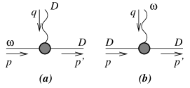
Vertex with $D$ off-shell. We start considering the $\omega DD$ vertex with one of the $D$ mesons off-shell (fig. 1-$a$). The three-point correlator is given by

$\displaystyle\Gamma_{\mu}^{(D)}(p,p^{\prime},Q)=\int d^{4}x\,d^{4}y\,e^{ip^{\prime}x}e^{-iqy}\Gamma_{\mu}^{(D)}(x,y)\,\,,$ (1)

where $\Gamma_{\mu}^{(D)}(x,y)=\langle 0|\mbox{T}\{j_{D}(x)j^{\dagger}_{D}(y)j^{\dagger}_{\mu}(0)\}|0\rangle$; with the currents given by $j_{D}=i\bar{u}\gamma_{5}c$ for $D$ and $j_{\mu}=\bar{u}\gamma_{\mu}u$ for $\omega$.

In the QCD side we perform the operator product expansion (OPE) [17] of the correlator $\Gamma_{\mu}^{(D)}(x,y)$

$\displaystyle\Gamma_{\mu}^{(D)}(x,y)=\bar{A}_{\mu}.1+\bar{B}_{\mu}.\langle\bar{q}q\rangle+...$ (2)

where 1 is the identity operator, $\bar{A}_{\mu}(x,y)$ is the perturbative contribution, $\langle\bar{q}q\rangle$ is the quark condensate and $\bar{B}_{\mu}(x,y)$ is the respective coefficient. Next, we present the calculations of $\bar{A}_{\mu}(x,y)$ and $\bar{B}_{\mu}(x,y)$ with some detail.

$\displaystyle A_{\mu}(x,y)=\mbox{Tr}\left[S_{u,d}(-y)\gamma_{5}S_{c}(y-x)\gamma_{5}S_{u,d}(x-0)\gamma_{\mu}\right]~{},$ (3)

where $S_{u,d}$ is the light quark $u$ (or $d$) propagator and $S_{c}$ is the quark $c$ propagator. After Fourier transforming the propagators, defining the variables: $s=p^{2}$, $u=p^{\prime}\,{}^{2}$, $t=q^{2}$, using Cutkosky rules and some extensive calculation we get the dispersion relation111Notation: $A_{\mu}=\bar{A}_{\mu}\cdot 1$.

$\displaystyle A_{\mu}(p,p^{\prime},q)=-\frac{1}{4\pi^{2}}\,\int_{s_{min}}^{\infty}ds\int_{u_{min}}^{\infty}du\frac{\mathcal{D}_{\mu}^{(D)}}{(s-p^{2})(u-p^{\prime 2})}~{},$ (4)

with the double discontinuity written as

$$\mathcal{D}_{\mu}^{(D)}=\rho\,p_{\mu}+\rho^{\prime}\,p^{\prime}_{\mu}~{},$$ (5)

and the spectral densities given by:

$\displaystyle\rho=-\frac{3}{2}\frac{(u-m_{c}^{2})}{\sqrt{\lambda(s,t,u)}}-\frac{6}{\pi}F\,,\,\,\rho^{\prime}=\,\,\frac{3}{2}\frac{s}{\sqrt{\lambda(s,t,u)}}-\frac{6}{\pi}G~{},$ (6)

with

$\displaystyle F$ $\displaystyle=$ $\displaystyle\frac{\pi}{8}\frac{(s-t-u+2m_{c}^{2})}{\sqrt{\lambda(s,t,u)}}\left[1-\frac{(s-t-u+2m_{c}^{2})(s-t+u)}{\lambda(s,t,u)}\right],$
$\displaystyle G$ $\displaystyle=$ $\displaystyle\frac{\pi}{4}\frac{s(s-t-u+2m_{c}^{2})^{2}}{\lambda^{3/2}(s,t,u)}\,\,,$ (7)

where $\lambda$ is the kinematical function: $\lambda(x,y,z)=(x-y-z)^{2}-4yz$

The integration limits of eq. (4) ($s_{min}$ and $u_{min}$) are determined from the conditions:

$\displaystyle s\geq 0\,,\quad u$ $\displaystyle\geq$ $\displaystyle t$
$\displaystyle(s-t-u+2m_{c}^{2})^{2}$ $\displaystyle\leq$ $\displaystyle\lambda(s,t,u)\,\,.$ (8)

We go to the Euclidean space with the transformations: $p^{2}\rightarrow-P^{2}$, $p^{\prime 2}\rightarrow-P^{\prime 2}$ and $q^{2}=t\rightarrow-Q^{2}$. And after performing the double Borel transform in $P$ and $P^{\prime}$, we obtain:

$\displaystyle\mathcal{B}_{P^{2}}\left[\mathcal{B}_{P^{\prime 2}}[A_{\mu}]\right]=-\frac{1}{4\pi^{2}}\,\int_{s_{min}}^{\infty}ds\int_{u_{min}}^{\infty}du\,\mathcal{D}_{\mu}^{(D)}\,e^{-s/M^{2}}e^{-u/M^{\prime 2}}~{}.$ (9)

Now we consider the non-perturbative contributions. Here we shall concentrate only in the quark condensate contribution. The first contribution is 222Notation: $B_{\mu}=\bar{B}_{\mu}\cdot\langle\bar{q}q\rangle$.:

$\displaystyle B_{\mu}^{(1)}(p,p^{\prime},q)=\int d^{4}xd^{4}ye^{ip^{\prime}x}e^{-iqy}B_{\mu}^{(1)}(x,y)~{},$ (10)

where

$\displaystyle B_{\mu}^{(1)}(x,y)=\mbox{Tr}\left[\left(-\frac{1}{12}\langle\bar{q}q\rangle\right)~{}.\gamma_{5}S_{c}(y-x)\gamma_{5}S_{u,d}(x)\gamma_{\mu}\right]\,,\,\,$ (11)

After some trivial manipulation we get

$$B_{\mu}^{(1)}(p,p^{\prime},q)=\frac{m_{c}\,p_{\mu}}{p^{2}(q^{2}-m_{c}^{2})}\,\langle\bar{q}q\rangle~{}.$$ (12)

It is not difficult to see that after going to the Euclidean space and taking the double Borel transform this contribution vanishes.

The second contribution is

$\displaystyle B_{\mu}^{(2)}(x,y)=\mbox{Tr}\left[S_{u,d}(-y)\gamma_{5}S_{c}(y-x)~{},\gamma_{5}\left(-\frac{1}{12}\langle\bar{q}q\rangle\right)\gamma_{\mu}\right]~{},$ (13)

that results in

$$B_{\mu}^{(2)}(p,p^{\prime},q)=\frac{-m_{c}\,p_{\mu}}{p^{2}(p^{\prime 2}-m_{c}^{2})}\,\langle\bar{q}q\rangle~{}.$$ (14)

Going to the Euclidean space and taking the double Borel transform we get

$\displaystyle\mathcal{B}_{P^{2}}\left[\mathcal{B}_{P^{\prime 2}}[B_{\mu}^{(2)}]\right]=-m_{c}\langle\bar{q}q\rangle e^{-m_{c}^{2}/M^{\prime 2}}p_{\mu}\,.$ (15)

There is also a numerically negligible contribution from the charm condensate, which we will not take into account in this calculation.

After the double Borel transformation the correlator (1), in the phenomenological side, can be written as

$\displaystyle\mathcal{B}_{P^{2}}\left[\mathcal{B}_{P^{\prime 2}}[\Gamma_{\mu}^{(D)}(p,p^{\prime},Q)|_{phen}]\right]=-\left(\frac{m_{D}^{2}f_{D}}{m_{c}}\right)^{2}\,m_{\omega}\,f_{\omega}\,\frac{g_{\omega DD}^{(D)}(Q^{2})}{m_{D}^{2}+Q^{2}}$
$\displaystyle\times e^{-m_{\omega}^{2}/M^{2}}e^{-m_{D}^{2}/M^{\prime 2}}\left(-2p^{\prime}_{\mu}+\frac{m_{D}^{2}+m_{\omega}^{2}+Q^{2}}{m_{\omega}^{2}}p_{\mu}\right)+\mathcal{B}_{P^{2}}\left[\mathcal{B}_{P^{\prime 2}}[\mbox{HR}]\right]~{},$ (16)

where $g_{\omega DD}^{(D)}$ is the $\omega DD$ vertex, $m_{\mbox{M}}$ and $f_{\mbox{M}}$ are, respectively, the mass and the decay constant of meson M ($\omega$ or $D$). HR represents the higher masses (continuum) resonances, whose contribution will be discussed below.

One important thing to be considered is the model to be adopted for the spectral density $\rho_{\mu}^{HR}(s,t,u)$ function (HR term in the phenomenological side). We should remember that the interpolating fields couple not only with the fundamental state but also with all particles with the same quantum numbers. We should also consider the contribution of those states in the phenomenological side. Admitting the quark–hadron duality, one assumes in general

$$\rho_{\mu}^{(HR)}(s,t,u)\approx\rho_{\mu}^{(OPE)}(s,t,u)\,\theta(s-s_{0})\,\theta(u-u_{0})\quad,$$ (17)

where $s_{0}$ and $u_{0}$ are the continuum thresholds.

Proceeding this way, we have after the Borel transformation:

$\displaystyle\mathcal{B}_{P^{2}}\left[\mathcal{B}_{P^{\prime 2}}[HR]\right]=-\frac{1}{4\pi^{2}}\,\int_{s_{0}}^{\infty}ds\int_{u_{0}}^{\infty}du\,\rho_{\mu}^{(OPE)}(s,t,u)\,e^{-s/M^{2}}\,e^{-u/M^{\prime 2}}~{}.$ (18)

In the case under consideration, it is not difficult to see that $\rho_{\mu}^{(OPE)}(s,t,u)\rightarrow\mathcal{D}_{\mu}^{(D)}(s,t,u)$. Now we have all ingredients for computing of $g_{\omega DD}^{(D)}(Q^{2})$ 333The superscript $(D)$ indicates that $D$ is off-shell. from the sum rule: (9) + (15) = (16).

Vertex with $\omega$ off-shell. Now let us consider the case when the $\omega$ meson is off-shell (fig. 1-$b$). We follow a similar procedure of the previous section. The three-point correlator is written as

$$\Gamma_{\mu}^{(\omega)}(x,y)=\langle 0|T{j_{D}(x)\,j^{\dagger}_{\mu}(y)\,j^{\dagger}_{D}(0)}|0\rangle\,\,.$$ (19)

For the perturbative contribution $A_{\mu}^{(\omega)}$, we obtained the double discontinuity $\mathcal{D}_{\mu}^{(\omega)}(s,u,t)=\rho(s,t,u).p_{\mu}+\rho^{\prime}(s,t,u)p^{\prime}_{\mu}$, with the the spectral densities:

$\displaystyle\rho(s,t,u)$ $\displaystyle=$ $\displaystyle+3\,\frac{(s-u-t)}{\lambda^{3/2}(s,u,t)}\,\,.[m_{c}^{2}(m_{c}^{2}-s-u+t)+su]$ (20)
$\displaystyle\rho^{\prime}(s,t,u)$ $\displaystyle=$ $\displaystyle-3\,\frac{(s-u+t)}{\lambda^{3/2}(s,u,t)}\,\,.[m_{c}^{2}(m_{c}^{2}-s-u+t)+su]~{}.$ (21)

The light quark condensate contributions ($B_{\mu}$) vanishes after double Borel transformation.

In the phenomenological side, the correlator (after double Borel transformation) is given by

$\displaystyle\mathcal{B}_{P^{2}}\left[\mathcal{B}_{P^{\prime 2}}[\Gamma_{\mu}^{(\omega)}|_{phen}]\right]=-\left(\frac{m_{D}^{2}f_{D}}{m_{c}}\right)^{2}\,m_{\omega}\,f_{\omega}\,\frac{g_{\omega DD}^{(\omega)}(Q^{2})}{m_{\omega}^{2}+Q^{2}}$
$\displaystyle\times e^{-m_{D}^{2}/M^{2}}e^{-m_{D}^{2}/M^{\prime 2}}\left(p^{\prime}_{\mu}+p_{\mu}\right)+\mathcal{B}_{P^{2}}\left[\mathcal{B}_{P^{\prime 2}}[\mbox{HR}]\right]\,.$ (22)

Now it is straightforward to construct the sum rules and to calculate the value of vertex form factor $g_{\omega DD}$.

Decay constants and thresholds. In the numerical evaluation of sum rules one can take into account the dependence of the decay constants with the Borel mass. In general this procedure improves the stability of the vertex sum rules with respect to the increasing of Borel mass. From the sum rules for the correlators of the mesons we obtained the decay constants as functions of the Borel mass:

$\displaystyle f_{\omega}^{2}(M^{2})$ $\displaystyle=$ $\displaystyle\left[\frac{M^{2}}{4\pi^{2}}(1-e^{-s_{0}/M^{2}})+2\frac{m_{q}\langle\bar{q}q\rangle}{M^{2}}\right]e^{m_{\omega}^{2}/M^{2}}~{},$ (23)
$\displaystyle f_{D}^{2}(M^{2})$ $\displaystyle=$ $\displaystyle\frac{m_{c}^{2}}{m_{D}^{4}}\left[\frac{3}{8\pi^{2}}\int_{m_{c}^{2}}^{s_{0}}ds\frac{(s-m_{c}^{2})^{2}}{s}e^{-s/M^{2}}-m_{c}\langle\bar{q}q\rangle e^{-m_{c}^{2}/M^{2}}\right]e^{m_{D}^{2}/M^{2}}$ (24)

As a common practice one usually assumes for the continuum threshold: $s_{0}=(m_{r}+\Delta_{r})^{2}$, where $m_{r}$ is the mass of the ground state resonance and $\Delta_{r}\sim 0.5-0.6$GeV. For consistency we verified that the value of $\Delta_{r}$ above is suitable, at least for $\omega$ and $D$ mesons. Such verification can be done once $f_{r}(M^{2})$ (actually $f_{r}(M^{2},s_{0})$) stabilizes fast enough with growth of $M^{2}$. Then we assume that $f_{r}(M^{2}\rightarrow\infty,s_{0})=f_{r}(s_{0})$ tends to the phenomenological (experimental) value of $f_{r}$.

For instance, in the case of the $\omega$ meson we can observe from (23):

$$f_{\omega}^{2}(M^{2}\rightarrow\infty,s_{0})\rightarrow\frac{s_{0}}{(2\pi)^{2}}=\frac{(m_{\omega}+\Delta_{\omega})^{2}}{(2\pi)^{2}}\,\,,$$ (25)

assuming $f_{\omega}^{(exp)}\approx 0.20$GeV and $m_{\omega}\approx 0.78$GeV, we obtain $\Delta_{\omega}\approx 0.48$GeV.

Repeating a similar calculation for eq. (24) with: $f_{D}\approx 0.17$GeV, $m_{D}\approx 1.9$GeV, $m_{c}\approx 1.2$GeV and $\langle\bar{q}q\rangle\approx(-0.23$GeV$)^{3}$, we estimate $\Delta_{D}\approx 0.53$GeV. We have seen that $\Delta_{r}\approx 0.6$GeV led to better stability of sum rules for larger values of Borel mass.

3 Numerical results and discussions

As one can observe, in the sum rules above we have two structures: one related to $p_{\mu}$ and other related to $p^{\prime}_{\mu}$. For $D$ off-shell the last structure is more stable (with respect to Borel mass) than the first one 444 On the other hand, for $\omega$ off–shell one can see that both structures are equal.. Therefore we concentrated our efforts in the analysis of $p^{\prime}_{\mu}$ structure.

The first step of the numerical analysis is to consider the behavior of the form factor vertex with respect to the variations of Borel masses. One important point that appears in this step is how to handle with the Borel masses $M$ and $M^{\prime}$. It is more or less intuitive that the Borel mass must be of the same order of magnitude of the mass of the corresponding particle. Then, for $D$ off–shell, we take the ratio $M/M^{\prime}\approx m_{\omega}/m_{D}$, and for $\omega$ off–shell we have $M/M^{\prime}\approx m_{D}/m_{D}$.

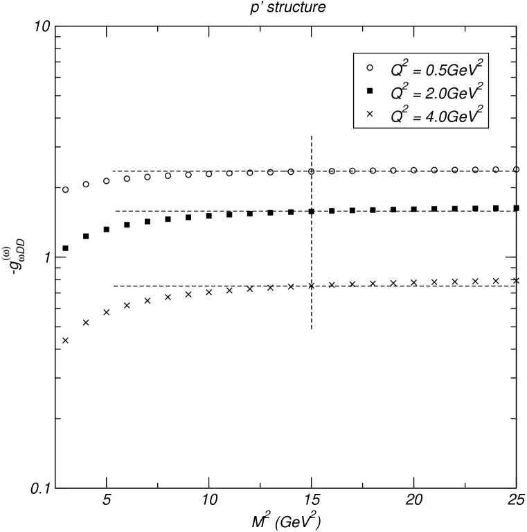
In fig. 2 we show the curves corresponding to $g_{\omega DD}^{(\omega)}$ as function of Borel mass for some fixed values of $Q^{2}$. We can note that $g_{\omega DD}^{(\omega)}$ stabilizes for $M^{2}\gtrsim 15$GeV2. A similar analysis is performed for $D$ off–shell, and we noted that $g_{\omega DD}^{(D)}$ stabilizes for $M^{2}\gtrsim 10$GeV2.

Refer to caption
Figure 2: Behavior of $(-g_{\omega DD}^{(\omega)})$ with $M^{2}$ for some fixed values of $Q^{2}$.

The second step is to fix the Borel mass in values for which the vertex form factor stabilizes, and study its dependence with $Q^{2}$. In figure 3 we plot our results for both situations: $D$ off–shell with $M^{2}=10$GeV2 ($\Box$) and $\omega$ off–shell $M^{2}=15$GeV2 ($\bullet$).

Refer to caption
Figure 3: Behavior of $(-g_{\omega DD}(Q^{2}))$ for $\omega$ and $D$ off–shell ($p^{\prime}$ structure).

We fitted some functions to the curves of figure 3. For $\omega$ off–shell we found:

$$-g_{\omega DD}^{(\omega)}(Q^{2})\approx 2.9\,e^{-Q^{2}/3.2}\,,$$ (26)

and for $D$ off–shell

$$-g_{\omega DD}^{(D)}(Q^{2})\approx\frac{31}{Q^{2}+11}\,.$$ (27)

From these fits we can estimate $g_{\omega DD}\approx-2.9$ at zero momentum transfer, which perfectly agrees with the result of VMD model.

In conclusion, we should say that the use of QCD Sum Rules approach to evaluate the $g_{\omega DD}$ vertex is completely acceptable and demostrates that it is still an open way to investigate other important hadronic quantities related with the formation of the quark-gluon plasma.

Acknowledgements

We thank CAPES (LBH) and FAPESP (AM and RSMC) for financial support. RSMC thanks T. Frederico for useful suggestions and UNESP - Itapeva for hospitality. AM thanks M. Chiapparini for discussions.

References

  • [1] T. Matsui, H. Satz, Phys. Lett. B 187 (1986) 416; R. Vogt, Phys. Rep. 310 (1999) 197.
  • [2] For recent review see B. Müller nucl-th/0508062.
  • [3] See for instance: R. S. Azevedo, F. S. Navarra and M. Nielsen, Acta Phys. Hung. A 24 (2005) 253; R. S. Azevedo, M. Nielsen, Phys. Rev. C 69 (2004) 035201.
  • [4] For experimental dicussion see S. Bianco hep-ex/0512073.
  • [5] S. G. Matinyan and B. Müller, Phys. Rev. C 58 (1998) 2994.
  • [6] K. Haglin, Phys. Rev. C 61 (2000) 031902.
  • [7] Z. Lin, C. M. Ko, Phys. Rev. C 62 (2000) 034903.
  • [8] F. Klingl, N. Kaiser and W. Weise, Z. Phys. A 356 (1996) 193.
  • [9] M. A. Shifman, A. I. Vainshtein, V. I. Zakharov, Nucl. Phys. B 147 (1979) 385; Nucl. Phys. B 147 (1979) 448.
  • [10] K.-C. Yang, W.-Y. P. Hwang, E. M.  Henley, L. S.  Kisslinger, Phys. Rev. D 47 (1993) 3001.
  • [11] H. Rubinstein, S. Yazaki, L. J.  Reinders, Phys. Rep. 127 (1985) 1.
  • [12] B. L. Ioffe and A. V. Smilga, Nucl. Phys. B 216 (1983) 373.
  • [13] B. L. Ioffe and A. V. Smilga Nucl. Phys. B 232 (1984) 109.
  • [14] P. Colangelo, A. Khodjamirian, hep-ph/0010175.
  • [15] R. D. Matheus, F. S. Navarra, M. Nielsen and R. Rodrigues da Silva, Phys. Lett. B 541(2002) 265.
  • [16] M. E. Bracco, M. Chiapparini, A. Lozea, F. S. Navarra and M. Nielsen, Phys. Lett. B 521 (2001) 1.
  • [17] T. Muta, Foundations of Quantum Chromodynamics, World Scientific, Singapore, (1987).