hep-ph/0612119
KA-TP-12-2006

Abstract

Slepton pairs can be produced in vector-boson fusion processes at hadron colliders. The next-to-leading order QCD corrections to the electroweak production cross section for $pp\rightarrow\tilde{\ell}^{+}\tilde{\ell}^{-}+2$ jets at order $\alpha_{s}\alpha^{4}$ have been calculated and implemented in a NLO parton-level Monte Carlo program. Numerical results are presented for the CERN Large Hadron Collider

PACS Nos: 11.10.Gh, 12.60.Jv, 14.80.Ly

Key Words: QCD corrections, Beyond Standard Model, Supersymmetry Phenomenology

Introduction:

Among the primary goals of the CERN Large Hadron Collider (LHC) are the discovery of the Higgs boson, thus shedding light on the yet unexplored mechanism of electroweak (EW) symmetry breaking, and the search for physics beyond the standard model. Within the area of Higgs boson studies, vector-boson fusion (VBF) processes have emerged as being highly promising for revealing information on the symmetry breaking sector [1]. The prototypical process is $qq\to qqH$, which proceeds via $t$-channel $W$ or $Z$ exchange. The two scattered quarks emerge as forward and backward jets (called tagging jets) which provide a characteristic signature for VBF and allow to significantly suppress backgrounds. As a result, VBF searches are expected to lead to quite clean Higgs boson signals.

A natural question is whether vector boson fusion is a useful tool also for the study of other signals of new physics. Some recent work has indicated the effectiveness of VBF channels in the context of new physics searches, particularly for new particles that do not interact strongly. Perhaps the best example [2] is afforded by supersymmetric theories, wherein conventional search strategies for neutralinos and charginos may run into difficulty at the LHC, for a significant part of the parameter space. The possibility of a slepton search has been studied for vector-boson fusion as well [3]. A more recent study [4] on VBF slepton production using Smadgraph arrived at a substantially smaller cross-section, however, which is partly caused by large cancellations among VBF-type diagrams and bremsstrahlung diagrams at the Born level.

The discrepancies between these previous results lead us to a recalculation of the slepton pair-production cross section in VBF. The relevant Feynman graphs for this process are depicted in Fig. 1 for the tree level contributions. In this approximation, we confirm the new results of Ref. [4]. In addition, we also perform a calculation of the NLO QCD corrections to this VBF process. The NLO calculation closely follows previous calculations for $Hjj$ and $Zjj$ production in VBF in Refs. [5, 6]. It uses the Catani-Seymour subtraction scheme [7] for implementing the real and virtual NLO contributions in the form of a fully flexible parton level Monte Carlo program.

1.5 0.7                       

Figure 1: Generic LO parton level diagrams leading to slepton pair-production through electroweak VBF at hadron colliders.

Calculation:

The Feynman graphs contributing to $pp\rightarrow\tilde{\ell}^{+}\tilde{\ell}^{-}+2$ jets at tree level are indicated in Fig. 1. Considering the possible choices of external quarks or anti-quarks, the sub-processes can be grouped into neutral-current (NC) processes, like $uc\rightarrow uc\tilde{\ell}^{+}\tilde{\ell}^{-}$, and charged-current (CC) processes, like $us\rightarrow dc\tilde{\ell}^{+}\tilde{\ell}^{-}$. For the purpose of calculating the virtual QCD corrections, the Feynman graphs are divided into Compton scattering type graphs, as in Fig. 1(a), and the VBF type graphs as in Fig. 1(b-e). The first class (Fig. 1(a) and three additional bremsstrahlung diagrams, with the vector boson radiated at the position of the blobs) corresponds to the emission of the external vector boson from one of the two quark lines. The VBF graphs represent $VV\rightarrow\tilde{\ell}^{+}\tilde{\ell}^{-}$. Here, V stands for a $t$-channel $\gamma$, $Z$ or $W$ boson. For selectron or smuon production one expects a negligible contribution from Fig. 1(b). We do include this Higgs exchange contribution for stau pair production, however, anticipating strong enhancements of the couplings to the Higgs bosons at large $\tan\beta$.

Contributions from anti-quark initiated $t$-channel processes such as $\bar{u}c\rightarrow\bar{u}c\tilde{\ell}^{+}\tilde{\ell}^{-}$, which emerge from crossing the above processes, are fully taken into account. On the other hand, two additional classes of diagrams which can appear in case of identical quark flavors, are simplified in our calculation. The first concern $s$-channel exchange diagrams, where both virtual vector bosons are time-like. These diagrams correspond to vector boson pair production with subsequent decay of one neutral vector boson to $\tilde{\ell}^{+}\tilde{\ell}^{-}$ while the other one decays into a quark-antiquark pair. These contributions can be safely neglected in the phase-space region where VBF can be observed experimentally, with widely-separated quark jets of large invariant mass. The second class corresponds to $u$-channel exchange diagrams which are obtained by the interchange of identical final state (anti)quarks. Their interference with the $t$-channel diagrams is strongly suppressed for typical VBF cuts and therefore neglected in our calculation. Color suppression further reduces any interference terms.

Throughout our calculation, fermion masses are set to zero and external b- and t-quark contributions are neglected. For the Cabibbo-Kobayashi-Maskawa matrix $V_{CKM}$, we use a diagonal form equal to the identity matrix. This yields the same results as a calculation using the exact $V_{CKM}$ when the summation over all quark flavors is performed.

The computation of NLO corrections is performed in complete analogy to Ref. [6]. For the real-emission contributions, we consider the diagrams with a final-state gluon by attaching the gluon to the quark lines in all possible ways. As a result one obtains two distinct, non-interfering color structures which correspond to gluon emission off the upper or off the lower quark line in Fig. 1. Subprocesses with an initial gluon are obtained by crossing the final state gluon on a given quark line with the incident quark or anti-quark of this same quark line. As a result only one color structure exists for initial gluons. The other color structure would correspond to an $s$-channel process of the type $gq\to VVq$, which has been neglected also at Born level.

All amplitudes are evaluated numerically using the amplitude techniques of Ref. [8]. The calculation is simplified by introducing the leptonic tensors $\Gamma^{\alpha}_{V}$ and $L^{\alpha\beta}_{VV}$, which describe the effective polarization vector of the final state decay $V(q)\to\tilde{\ell}^{-}(p_{1})\tilde{\ell}^{+}(p_{2})$,

$$\Gamma^{\alpha}_{V}(p_{1},p_{2})=\frac{g_{\tau}^{V\tilde{\ell}}}{(p_{1}+p_{2})^{2}-m^{2}_{V}+im_{V}\Gamma_{V}}(p_{1}-p_{2})^{\alpha}\;,$$ (1)

and the effective sub-amplitude for the process $V_{1}^{\alpha}V_{2}^{\beta}\to\tilde{\ell}^{+}\tilde{\ell}^{-}$. The leptonic tensor $\Gamma^{\alpha}_{V}$ is common to real emission graphs and Born graphs appearing in the Catani-Seymour subtraction terms and needs to be calculated only once at a given phase space point, independent of the crossing of the colored partons. Similarly, $L^{\alpha\beta}_{VV}$ is only needed for two distinct momentum flows (gluon attached to the upper or to the lower quark line) at any phase space point. It is calculated in the complex-mass scheme [9] which implements the Breit-Wigner propagators of the resonant $Z$-boson in a gauge invariant way.

At NLO, we have to deal with singularities in the soft and collinear regions of phase space which are regularized in the dimensional-reduction scheme [10] with space-time dimension $d=4-2\epsilon$. The cancellation of these divergences with the respective poles from the virtual contributions is performed by introducing the counter terms of the dipole subtraction method [7]. Since these divergences only depend on the color structure of the external partons, the analytical form of subtraction terms and finite collinear pieces encountered for VBF slepton pair production, in terms of the respective Born amplitude, is identical to the ones given in Ref. [5].

The virtual corrections to the amplitudes arise from a virtual gluon emitted and re-absorbed by either the upper fermion line or by the lower fermion line. For both contributions the resulting virtual amplitude, ${\cal M}_{V}$, can be expressed in term of a divergent part, which is fully factorisable in terms of the original Born amplitude, ${\cal M}_{B}$, and a finite part, $\tilde{{\cal M}_{V}}$,

$${\cal M}_{V}={\cal M}_{B}\frac{\alpha_{s}(\mu_{R})}{4\pi}C_{F}\left(\frac{4\pi\mu_{R}^{2}}{Q^{2}}\right)^{\epsilon}\Gamma(1+\epsilon)\left(-\frac{2}{\epsilon^{2}}-\frac{3}{\epsilon}+c_{virt}\right)+\tilde{{\cal M}_{V}}\;.$$ (2)

Here, the first term gets contributions from virtual QCD corrections to all types of Feynman graphs as in Fig. 1 but the finite second part originates from virtual QCD corrections to only those Feynman graphs where two electroweak bosons are attached to the same fermion line, as shown in Fig. 1(a). The full expression of this finite part can be expressed in terms of the finite parts of the Passarino-Veltman [11] $B_{0}$, $C_{0}$ and $D_{ij}$ functions and was given in Eq. (A1) of Ref. [6] for the analogous case of $V\to l^{+}l^{-}$ decay: simply replace one of the two polarization vectors $\epsilon_{i}^{\alpha}$ of Eq. (A1) by the slepton current $\Gamma^{\alpha}_{V}$ of Eq. (1).

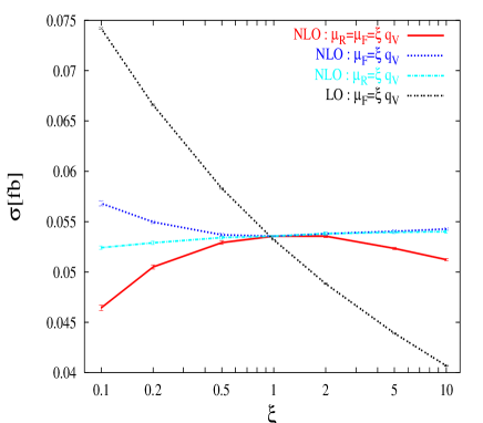
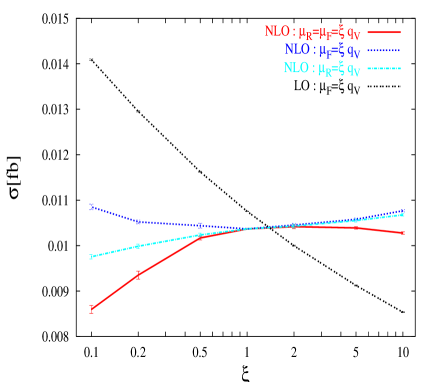
Figure 2: Scale dependence of the $pp\rightarrow\tilde{\ell}^{+}\tilde{\ell}^{-}jjX$ cross section at the LHC for (a) left-type slepton and (b) right-type slepton at NLO and LO with the cuts of Eqns.(3, 4). The slepton masses are $m_{\tilde{\ell}_{L}}=m_{\tilde{\ell}_{R}}=200$ GeV.

The results obtained for the Born amplitude, the real emission and the virtual corrections have been tested extensively. For the tree-level amplitudes (Born and real emission), we have performed a comparison to the fully automatically generated results provided by Smadgraph [4] and confirmed their equality numerically. We also checked the invariance of the Born cross-section under Lorentz transformations. Furthermore, gauge invariance has been confirmed for the external gluon, within the numerical accuracy of the program.

Results and Discussions:

The cross-section contributions discussed in the previous section are implemented in a fully-flexible parton-level Monte Carlo program for EW $\tilde{\ell}^{+}\tilde{\ell}^{-}jj$ production at NLO QCD accuracy. The program is very similar to the ones for Hjj, Vjj and VVjj production in VBF described in Refs. [5], [6] and [12]. We use the CTEQ6M parton distributions with $\alpha_{s}(m_{Z})=0.118$ at NLO, and CTEQ6L1 distributions for all LO cross sections. We chose $m_{Z}=91.188\;{\rm GeV}$, $m_{W}=80.423\;{\rm GeV}$ and $G_{F}=1.166\times 10^{-5}\;{\rm GeV}^{-2}$ as electroweak input parameters. Thereof, $\alpha_{QED}=1/132.54$ and $\sin^{2}{\theta_{W}}=0.22217$ are computed via LO electroweak relations. To reconstruct jets from final-state partons, the kT algorithm is used with resolution parameter D = 0.8 [13]. Throughout, we assume a pure $\ell\tilde{\chi}_{1}^{0}$ decay of the sleptons, whenever decay distributions are being discussed.

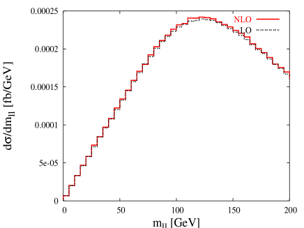
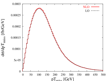
Figure 3: Distributions for (a) daughter lepton invariant mass $M_{ll}$ and (b) missing transverse momentum $pT_{miss}$ at NLO (solid red) and LO (dashed black). Left type slepton production in the SPS 1a scenario ($m_{\tilde{\ell}}=202\;{\rm GeV}$) is considered. Renormalization and factorization scales are taken as $\mu_{R}=\mu_{F}=q_{V}$.

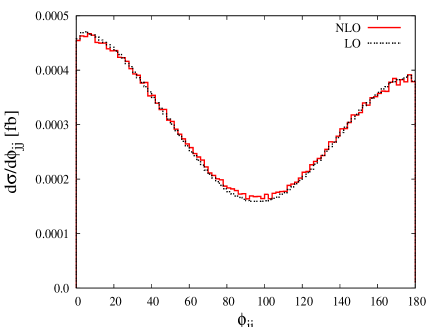
Figure 4: Distributions of the azimuthal angle between the two tagging jets , $\phi_{jj}$, at NLO (solid red) and LO (dashed black). Left type slepton production in SPS 1a scenario ($m_{\tilde{\ell}}=202\;{\rm GeV}$) is considered. Renormalization and factorization scales are taken as $\mu_{R}=\mu_{F}=q_{V}$.

Partonic cross sections are calculated for events with at least two hard jets, which are required to have

$$p_{T_{j}}\geq 20\;{\rm GeV},\qquad|y_{j}|\leq 4.5$$ (3)

Here $y_{j}$ denotes the rapidity of the (massive) jet momentum which is reconstructed as the four-vector sum of massless partons of pseudo-rapidity $|\eta|<5$. These cuts ensure a finite LO differential cross section for $\tilde{\ell}^{+}\tilde{\ell}^{-}jj$ production, since they enforce finite scattering angles for the two quark jets. The two reconstructed jets of highest transverse momentum are called ’tagging jets’. At LO, they are the final-state quarks which are characteristic of vector-boson fusion processes. Backgrounds to VBF are significantly reduced by requiring a large rapidity separation of the two tagging jets. We therefore impose the cut

$$\Delta y_{jj}=|y_{j_{1}}-y_{j_{2}}|>4.2$$ (4)

Within the above cuts we have calculated the $\tilde{\ell}^{+}\tilde{\ell}^{-}jj$ cross sections at LO and at NLO for the SPS 1a parameter point where slepton masses are given by $m_{\tilde{\ell}_{L}}$= 202 GeV, $m_{\tilde{\ell}_{R}}$= 144 GeV. This point can be parameterized by the mSUGRA model with $m_{0}=100$ GeV, $m_{1/2}=250$ GeV, $A_{0}=-100$ GeV, $\tan{\beta}=10$ and positive $\mu$ [14]. We find production cross sections of 0.0536 (0.0532) fb for $\tilde{\ell}_{L}$ production and 0.0242 (0.0249) fb for $\tilde{\ell}_{R}$ production at NLO (LO) when setting renormalization and factorization scales to $\mu_{R}=\mu_{F}=q_{V}$. Unfortunately, expected cross sections at the LHC are quite small in general, not exceeding 0.1 fb for slepton masses above 150 GeV for left-handed sleptons and for slepton masses above 80 GeV for right-handed sleptons. In order to compare $\tilde{\ell}_{L}$ and $\tilde{\ell}_{R}$ cross sections more directly, we have calculated their total production cross sections, within the above cuts, for a mass of 200 GeV in both cases. Fig. 2 illustrates the dependence of these total cross sections on the renormalization and factorization scales, $\mu_{R}$ and $\mu_{F}$, which are taken as multiples of the momentum transfers, $q_{V}$, of the $t$-channel electroweak bosons in Fig. 1, $\mu_{R}=\xi_{R}q_{V}$, $\mu_{F}=\xi_{F}q_{V}$. This choice takes into account that at both LO and NLO the VBF process can be viewed as a double deep inelastic scattering event, for which the momentum transfer carried by the exchanged electroweak boson is a natural scale choice. It leads to K-factors close to unity for both total cross sections and distributions.

The LO cross section, $\sigma_{LO}$, only depend on $\mu_{F}=\xi_{F}q_{V}$. By varying the scale factor $\xi_{F}=\xi$ in the range 0.1 - 10, the value of $\sigma_{LO}$ changes by around a factor of two, indicating a substantial theoretical uncertainty of the LO calculation. The strong scale dependence is reduced at NLO. For $\sigma_{NLO}$, we show three different cases: $\xi_{F}=\xi_{R}=\xi$ (solid red line), $\xi_{F}=\xi$, $\xi_{R}=1$ (dot-dashed blue line), and $\xi_{F}=1$, $\xi_{R}=\xi$ (dashed green line). The latter curve illustrates clearly the weak dependence of $\sigma_{NLO}$ on the renormalization scale, which can be understood from the fact that $\alpha_{s}(\mu_{R})$ enters only at NLO. Also the factorization-scale dependence of the full cross section is low. In our following study we fix the scales at $\mu_{F}=\mu_{R}=q_{V}$, unless noted otherwise.

Two examples for distributions are given in Fig. 3. We show the distributions for (a) the invariant mass, $M_{ll}$, of the two charged daughter leptons in the decay $\tilde{\ell}^{+}\tilde{\ell}^{-}\to l^{+}l^{-}{p_{T}}_{miss}$, and (b) the missing transverse momentum, ${p_{T}}_{miss}$. Results are shown at both LO and NLO and are virtually indistinguishable with the scale choice $\mu_{F}=\mu_{R}=q_{V}$. For the illustration in Fig. 3, left type slepton production ($pp\rightarrow\tilde{\ell}_{L}^{+}\tilde{\ell}_{L}^{-}jjX$) in the SPS 1a scenario ($m_{\tilde{\ell}}=202\;{\rm GeV}$) is considered.

Within the same set of model parameters, the distribution in the azimuthal angle between the two tagging jets, $\phi_{jj}$, is shown in Fig. 4. One finds a characteristic dip at $90^{0}$, a feature which otherwise is only found in $Hjj$ production when the Higgs boson couples to gauge bosons via a $HV_{\mu\nu}V^{\mu\nu}$ operator in the effective Lagrangian [15]. $Hjj$ or $Zjj$ production via VBF in the SM produces a fairly flat $\phi_{jj}$ distribution, while $Hjj$ production via gluon fusion exhibits a structure very similar to the one shown in Fig. 4. Since it has been suggested that the $\phi_{jj}$ distribution in VBF events be used in distinguishing SM Higgs couplings from anomalous couplings, the possibility that a dip at $90^{0}$ might also be produced by the production of two charged scalars should be kept in mind, should such a feature be discovered at the LHC.

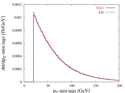
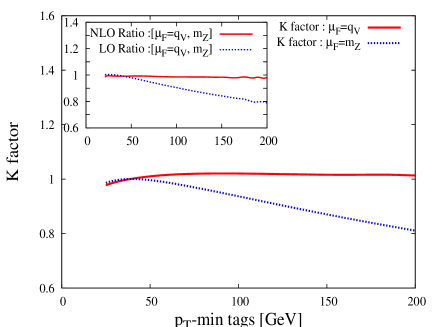
Figure 5: (a) Distribution of the minimum transverse momentum of the two tagging jets, $p_{T,min}(tags)$, at NLO (solid red) and LO (dashed black) for the scale choice $\mu_{R}=\mu_{F}=q_{V}$. (b) K factor as defined in Eq. (5) after fixing the factorization scale at the momentum transfer $\mu_{F}=q_{V}$ (solid red) and at $\mu_{F}=m_{Z}$ (dashed blue). The inset shows the ratio between these two choice of factorization scale at NLO (solid red) and at LO (dashed black). Left type slepton production in the SPS 1a scenario ($m_{\tilde{\ell}}=202\;{\rm GeV}$) is shown.

A distribution which distinguishes slepton pair production from many other VBF processes is the minimum transverse momentum of the two tagging jets, $d\sigma/dp_{T,min}(tags)$, which is depicted in Fig. 5(a). Due to a significant contribution from $t$-channel photon exchange, this distribution falls quite steeply. An even steeper fall-off is found for right type slepton production ($pp\rightarrow\tilde{\ell}_{R}^{+}\tilde{\ell}_{R}^{-}jjX$), which can be understood from the fact that $\tilde{\ell}_{R}$ has no coupling to the $W^{\pm,0}$ eigenstates.

The shape of the above distribution at LO can differ significantly from the respective NLO result when scales other than $\mu_{R}=\mu_{F}=q_{V}$ are used. This is emphasized in Fig. 5(b), where we show the dynamical K factor, defined as

$$K(x)=\frac{d\sigma_{NLO}/dx}{d\sigma_{LO}/dx}$$ (5)

for the two choices $\mu_{F}=q_{V}$ and $\mu_{F}=m_{Z}$ (and $\mu_{R}=q_{V}$ for the NLO curves in both cases). While the NLO cross sections differ very little when switching between the two scale choices (see inset), the effect on the LO cross sections is quite sizable, approaching a 20% effect at $p_{Tj}\approx 200$ GeV. This is to illustrate that the choice $\mu_{F}=q_{V}$ minimizes the NLO corrections in most distributions, by producing a LO prediction which is close to the true NLO result.

Summary and Conclusions:

In this paper we have presented results for EW slepton pair production at NLO QCD accuracy, obtained with a new parton-level Monte Carlo program. The integrated cross sections for this process are consistent with the results of Ref. [4] and show a very moderate K factor. While NLO results are quite stable against scale variations, LO results can change substantially. We find that the higher order QCD corrections are minimized by the scale choice $\mu_{F}=q_{V}$ at LO, where $q_{V}$ is the momentum transfer carried by the $t$-channel electroweak bosons.

A second observation concerns the distribution of the azimuthal angle separation between the two tagging jets in VBF events. The VBF production of two scalars, as considered here, produces the same type of dip at $90^{0}$ as is otherwise observed only for Higgs production with loop induced couplings to the fusing vector bosons.

Acknowledgments

P.K. would like to thank B. Jäger for many helpful discussions in the process of numerical calculation. This research was supported in part by the Deutsche Forschungsgemeinschaft under SFB/TR-9 “Computergestützte Theoretische Teilchenphysik”.

References

- [1] D. L. Rainwater and D. Zeppenfeld, JHEP 9712, 005 (1997) [arXiv:hep-ph/9712271]; D. L. Rainwater and D. Zeppenfeld, Phys. Rev. D 60, 113004 (1999) [Erratum-ibid. D 61, 099901 (2000)] [arXiv:hep-ph/9906218]; T. Plehn, D. L. Rainwater and D. Zeppenfeld, Phys. Rev. D 61, 093005 (2000) [arXiv:hep-ph/9911385]; S. Asai et al., Eur. Phys. J. C 32S2, 19 (2004) [arXiv:hep-ph/0402254].
- [2] A. Datta, P. Konar and B. Mukhopadhyaya, Phys. Rev. Lett. 88, 181802 (2002) [arXiv:hep-ph/0111012]; A. Datta, P. Konar and B. Mukhopadhyaya, Phys. Rev. D 65, 055008 (2002) [arXiv:hep-ph/0109071].
- [3] D. Choudhury, A. Datta, K. Huitu, P. Konar, S. Moretti and B. Mukhopadhyaya, Phys. Rev. D 68, 075007 (2003) [arXiv:hep-ph/0304192]; P. Konar and B. Mukhopadhyaya, Phys. Rev. D 70, 115011 (2004) [arXiv:hep-ph/0311347].
- [4] G. C. Cho, K. Hagiwara, J. Kanzaki, T. Plehn, D. Rainwater and T. Stelzer, Phys. Rev. D 73, 054002 (2006) [URL: http://www.ph.ed.ac.uk/~tplehn/smadgraph/] [arXiv:hep-ph/0601063].
- [5] T. Figy, C. Oleari and D. Zeppenfeld, Phys. Rev. D 68, 073005 (2003) [arXiv:hep-ph/0306109].
- [6] C. Oleari and D. Zeppenfeld, Phys. Rev. D 69, 093004 (2004) [arXiv:hep-ph/0310156].
- [7] S. Catani and M. H. Seymour, Nucl. Phys. B 485, 291 (1997) [Erratum-ibid. B 510, 503 (1997)] [arXiv:hep-ph/9605323].
- [8] K. Hagiwara and D. Zeppenfeld, Nucl. Phys. B 274, 1 (1986); K. Hagiwara and D. Zeppenfeld, Nucl. Phys. B 313, 560 (1989).
- [9] A. Denner, S. Dittmaier, M. Roth and D. Wackeroth, Nucl. Phys. B560, 33 (1999) [arXiv:hep-ph/9904472].
- [10] W. Siegel, Phys. Lett. B 84, 193 (1979); W. Siegel, Phys. Lett. B 94, 37 (1980).
- [11] G. Passarino and M. J. G. Veltman, Nucl. Phys. B 160, 151 (1979).
- [12] B. Jäger, C. Oleari and D. Zeppenfeld, JHEP 0607, 015 (2006) [arXiv:hep-ph/0603177]; B. Jäger, C. Oleari and D. Zeppenfeld, Phys. Rev. D 73, 113006 (2006) [arXiv:hep-ph/0604200].
- [13] S. Catani, Y. L. Dokshitzer and B. R. Webber, Phys. Lett. B 285, 291 (1992); S. Catani, Y. L. Dokshitzer, M. H. Seymour and B. R. Webber, Nucl. Phys. B 406, 187 (1993); S. D. Ellis and D. E. Soper, Phys. Rev. D 48, 3160 (1993) [arXiv:hep-ph/9305266].
- [14] B. C. Allanach et al., Eur. Phys. J. C 25, 113 (2002) [eConf C010630, P125 (2001)].
- [15] V. Del Duca, W. Kilgore, C. Oleari, C. Schmidt and D. Zeppenfeld, Nucl. Phys. B 616, 367 (2001) [arXiv:hep-ph/0108030]; T. Plehn, D. L. Rainwater and D. Zeppenfeld, Phys. Rev. Lett. 88, 051801 (2002) [arXiv:hep-ph/0105325]; V. Hankele, G. Klämke, D. Zeppenfeld, and T. Figy, Phys. Rev. D 74, 095001 (2006) [arXiv:hep-ph/0609075].