Abstract

Recent work in low energy pion physics is reviewed. One of the exciting new developments in this field is that simulations of QCD on a lattice now start providing information about the low energy structure of the continuum theory, for physical values of the quark masses. Although the various sources of systematic error yet need to be explored more thoroughly, the results obtained for the correlation function of the axial current with the quantum numbers of the pion already have important implications for the effective Lagrangian of QCD. The consequences for $\pi\pi$ scattering are discussed in some detail. The second part of the report briefly reviews recent developments in the dispersion theory of the scattering amplitude. One of the important results here is that the position of the lowest resonances of QCD can now be determined in a model independent manner and rather precisely. Beyond any doubt, the partial wave with $I=\ell=0$ contains a pole on the second sheet, not far from the threshold: the lowest resonance of QCD carries the quantum numbers of the vacuum.

Contribution to the proceedings of the workshop Chiral Dynamics,

Theory & Experiment, Durham/Chapel Hill, NC, USA, September 2006

1 Introduction

The pions are the lightest hadrons and we know why they are so light. Since the underlying approximate symmetry also determines their basic properties at low energy, the interaction among the pions is understood very well. In fact, in the threshold region, the $\pi\pi$ scattering amplitude is now known to an amazing degree of accuracy.[1] In particular, we know how to calculate the mass and width of the lowest resonance of QCD in a model independent manner.[2] The actual uncertainty in the pole position is smaller than the estimate given in the 2006 edition of the Review of Particle Physics,[3] by more than an order of magnitude.

The progress made in this field heavily relies on the fact that the dispersion theory of $\pi\pi$ scattering is particularly simple: the $s$-, $t$- and $u$-channels represent the same physical process. As a consequence, the scattering amplitude can be represented as a dispersion integral over the imaginary part and the integral exclusively extends over the physical region.[4] Throughout the following, I work in the isospin limit ($m_{u}=m_{d}=m$ and $e=0$), where the representation involves only two subtraction constants. These may be identified with the $S$-wave scattering lengths $a_{0}^{0},a_{0}^{2}$. The projection of the amplitude on the partial waves leads to a dispersive representation for these, the Roy equations. For a thorough discussion, I refer to ACGL.[5]

The pioneering work on the physics of the Roy equations was carried out more than 30 years ago.[6] The main problem encountered at that time was that the two subtraction constants occurring in these equations were not known: if the values of $a_{0}^{0}$, $a_{0}^{2}$ are contained in the so-called universal band – the region spanned by the two thick lines in figure 1 below – the Roy equations admit a solution. Since the data available at the time were consistent with a very broad range of $S$-wave scattering lengths, the Roy equation analysis was not conclusive.

2 Low energy theorems for the $S$-wave scattering lengths

The insights gained by means of chiral perturbation theory ($\chi$PT ) thoroughly changed the situation.[7] The corrections to Weinberg’s low energy theorems[8] for $a_{0}^{0},a_{0}^{2}$ (left dot in figure 1) have been worked out to first non-leading order[9] (middle dot) and those of next-to-next-to leading order are also known[10] (dot on the right). As demonstrated in CGL,[1] the chiral perturbation series converges particularly rapidly near the center of the Mandelstam triangle, so that very accurate predictions for the scattering lengths are obtained by matching the chiral and dispersive representations there.

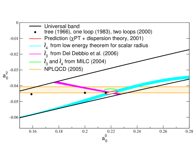
Figure 1: $S$ wave scattering lengths: theoretical results.

Using this method, the low energy theorems for $a_{0}^{0}$, $a_{0}^{2}$ may be brought to the form

$$\rule{14.22636pt}{0.0pt}2a_{0}^{0}+7a_{0}^{2} = -\,6\pi\left(\!\frac{M_{\pi}}{4\pi F_{\pi}}\!\right)^{\!\!4}\!\left(\bar{\ell}_{3}-\frac{193}{210}\right)+M_{\pi}^{4}\alpha_{3}+O(M_{\pi}^{6})\,,\hskip 34.14322pt(1a)$$

$$2a_{0}^{0}-5a_{0}^{2} = \frac{3M_{\pi}^{2}}{4\pi F_{\pi}^{2}}+24\pi\!\left(\!\frac{M_{\pi}}{4\pi F_{\pi}}\!\right)^{\!\!4}\left(\!\bar{\ell}_{4}-\frac{887}{840}\right)+M_{\pi}^{4}\alpha_{4}+O(M_{\pi}^{6})\,.\hskip 5.69046pt(1b)$$

While the chiral expansion of $a_{0}^{0},a_{0}^{2}$ starts at order $M_{\pi}^{2}$, with a term that is fixed by the pion decay constant, the combination $2a_{0}^{0}+7a_{0}^{2}$ vanishes at leading order. Two types of corrections occur at $O(M_{\pi}^{4})$: a contribution from the coupling constants $\bar{\ell}_{3},\bar{\ell}_{4}$ of the effective Lagrangian and one involving dispersion integrals, which I denote by $M_{\pi}^{4}\alpha_{3}$ and $M_{\pi}^{4}\alpha_{4}$, respectively (these also contain higher order contributions).

A representation similar to (1) was given earlier,[9] but there, the dispersion integrals $M_{\pi}^{4}\alpha_{3},M_{\pi}^{4}\alpha_{4}$ were evaluated at leading order, where they can be expressed in terms of the $D$-wave scattering lengths. The virtue of the above form of the low energy theorems is that (a) the neglected terms of order $M_{\pi}^{6}$ are much smaller than in the straightforward chiral perturbation series and (b) the dispersion integrals can be evaluated quite accurately, on the basis of the Roy equations. Since the integrals converge very rapidly, they depend almost exclusively on the scattering lengths $a_{0}^{0},a_{0}^{2}$. In the vicinity of the physical values, the linear representations

$$\rule{14.22636pt}{0.0pt}M_{\pi}^{4}\alpha_{3} = 0.135+0.77\,(a^{0}_{0}-0.220)-1.50\,(a^{2}_{0}+0.0444)\,,\hskip 47.51604pt(2a)$$

$$M_{\pi}^{4}\alpha_{4} = 0.061+0.48\,(a^{0}_{0}-0.220)-0.26\,(a^{2}_{0}+0.0444)\,,\hskip 48.36958pt(2b)$$

provide an excellent approximation. For a detailed discussion, in particular also of the uncertainties, I refer to CGL. The estimates given there show that the contributions of order $M_{\pi}^{6}$ in (1a) generate a correction of order 0.002, while those in equation (1b) are of order 0.003.

The low energy theorems (1) show that the $S$-wave scattering lengths are related to the coupling constants $\bar{\ell}_{3}$ and $\bar{\ell}_{4}$. Indeed, these play a central role in the effective theory, because they determine the dependence of $M_{\pi}$ and $F_{\pi}$ on the quark mass at first non-leading order: the expansion of $M_{\pi}^{2}$ and $F_{\pi}$ in powers of the quark mass starts with

$$M_{\pi}^{2}=M^{2}\{1+\mbox{$\frac{1}{2}$}\,x\,\bar{\ell}_{3}+O(x^{2})\}\,,\hskip 14.22636ptF_{\pi}=F\{1+x\,\bar{\ell}_{4}+O(x^{2})\}\,,$$ (3)

where $M^{2}=2Bm$ is proportional to the quark mass, $F$ is the value of the pion decay constant in the chiral limit, and $x\equiv M^{2}\!/(16\pi^{2}F^{2})$. A crude estimate for $\bar{\ell}_{3}$ can be obtained from the mass spectrum of the pseudoscalar octet: $\bar{\ell}_{3}=2.9\pm 2.4$.[9] For $\bar{\ell}_{4}$, an analogous estimate ($\bar{\ell}_{4}=4.3\pm 0.9$) follows from the experimental value of the ratio $F_{K}/F_{\pi}$. The low energy theorem for the radius of the scalar pion form factor yields a more accurate result: $\bar{\ell}_{4}=4.4\pm 0.2$.[11] The error is smaller here, because the theorem holds within SU(2)$\times$SU(2), so that an expansion in the mass of the strange quark is not necessary. The small ellipse in figure 1 shows the prediction for the scattering lengths obtained in CGL with these values of $\bar{\ell}_{3}$ and $\bar{\ell}_{4}$ (since the residual errors are small, the corrections of order $M_{\pi}^{6}$ are not entirely negligible – the curve shown includes an estimate for these).

The narrow strip that runs near the lower edge of the universal band indicates the region allowed if the coupling constant $\bar{\ell}_{3}$ is treated as a free parameter, while $\bar{\ell}_{4}$ is fixed with the scalar radius, like for the ellipse. By construction, the upper and lower edges of the strip are tangent to the ellipse. As implied by equations (1b) and (2b), the strip imposes an approximately linear correlation between the two scattering lengths – a curvature becomes visible only in the region where the theoretical prediction would be totally wrong.

3 Lattice results

On the lattice, dynamical quarks can now be made sufficiently light to establish contact with the effective low energy theory of QCD. In particular, the MILC collaboration obtained an estimate for the coupling constants $L_{4},L_{5},L_{6},L_{8}$ of the effective chiral SU(3)$\times$SU(3) Lagrangian.[12] Using standard one loop formulae,[13] these results lead to $\bar{\ell}_{3}=0.8\pm 2.3$ and $\bar{\ell}_{4}=4.0\pm 0.6$. In the plane of the two $S$-wave scattering lengths, the MILC results select the region indicated by the second ellipse shown in figure 1, which is slightly larger. It would be worthwhile to analyze these data within SU(2)$\times$SU(2), in order to extract the constants $\bar{\ell}_{3}$ and $\bar{\ell}_{4}$ more directly. The one loop formulae of SU(3)$\times$SU(3) are subject to inherently larger corrections from higher orders, so that the results necessarily come with a larger error (note that, at the present state of the art, the analysis of the lattice data relies on the one loop formulae).

The second narrow strip shown in the figure is obtained by treating $\bar{\ell}_{4}$ as an unknown. Instead of showing the region that belongs to the value of $\bar{\ell}_{3}$ used for the ellipse, I am taking $\bar{\ell}_{3}$ from a lattice study, which appeared very recently.[14] In that work, the dependence of $M_{\pi}^{2}$ and $F_{\pi}$ on the quark mass is investigated for two flavours of light Wilson quarks. The results for $M_{\pi}^{2}$ are consistent with one loop $\chi$PT . With $M_{K\mbox{\tiny ref}}=495$ MeV, the result $\hat{\ell}_{3}=0.5(5)(1)$ implies $\bar{\ell}_{3}=3.0\pm 0.5\pm 0.1$. Since this is close to the center of the estimated range, the strip runs through the middle of the ellipse. Taken at face value, the uncertainty in the lattice result for $\bar{\ell}_{3}$ is four times smaller than the one in the estimate $\bar{\ell}_{3}=2.9\pm 2.4$, obtained from the SU(3) mass formulae for the pseudoscalars, more than 20 years ago.[9] While the width of the ellipse is dominated by the uncertainty in the value used for $\bar{\ell}_{3}$, those associated with the higher order contributions and with the phenomenological uncertainties in the dispersion integrals do affect the width of the strip belonging to the value of Del Debbio et al. – this is why the higher precision for $\bar{\ell}_{3}$ reduces the width by less than a factor of four.

The coupling constants depend logarithmically on the pion mass:

$$\bar{\ell}_{3}=\ln\frac{\Lambda_{3}^{2}}{M_{\pi}^{2}}\,,\hskip 14.22636pt\bar{\ell}_{4}=\ln\frac{\Lambda_{4}^{2}}{M_{\pi}^{2}}\,,$$ (4)

so that their value changes if the quark mass is varied. The quoted value for $\bar{\ell}_{3}$ corresponds to $\Lambda_{3}\simeq 560$ MeV. For $M_{\pi}<\Lambda_{3}$, the curvature term is positive and reaches a maximum at $M_{\pi}=\Lambda_{3}/\sqrt{e}\simeq 340$ MeV. Even there, $\frac{1}{2}x\,\bar{\ell}_{3}$ is less than 0.05, so that $M_{\pi}^{2}/m$ is indeed nearly a constant. Although more work is needed to clarify all sources of uncertainty, the calculation beautifully confirms that, to a very good approximation, $M_{\pi}^{2}$ is linear in the quark mass. Hence the quark condensate indeed represents the leading order parameter of the spontaneously broken symmetry.[15] The same lattice data also yield information about the dependence of $F_{\pi}$ on the quark mass, but the comparison with the one loop formula of $\chi$PT is not conclusive in this case: the result for $\bar{\ell}_{4}$ depends on how the data are analyzed.[14]

The quark mass dependence of $M_{\pi}$ and $F_{\pi}$ is also being studied by the European Twisted Mass Collaboration. The preliminary results for the relevant effective coupling constants read $\bar{\ell}_{3}=3.5$ and $\bar{\ell}_{4}=4.4$. A thorough analysis of the uncertainties is under way.[16]

Finally, I mention that the scattering length of the exotic $S$-wave, $a_{0}^{2}$, can be determined directly, from the volume dependence of the energy levels occurring on the lattice. The horizontal band shown in figure 1 indicates the result obtained in this way by NPLQCD.[17] It is also consistent with the other pieces of information shown in the figure. Although possible in principle, it is difficult to extend this method to the isoscalar channel.

4 Experiment

Since the pions are not stable, they first need to be produced before they can be studied, so that the experimental information is of limited accuracy. Moreover, there are inconsistencies among the various data sets. One of the problems is that, in most production experiments, the two pions in the final state are accompanied by other hadrons. I know of three exceptions: production via photons in $e^{+}e^{-}$ collisions or via $W$-bosons in the decays $\tau^{\pm}\rightarrow\nu\,\pi^{\pm}\pi^{0}$ and $K\rightarrow e\nu\pi\pi$. The first two yield excellent information about the electromagnetic and weak vector form factors of the pion and hence also about the $P$-wave $\pi\pi$ phase shift.

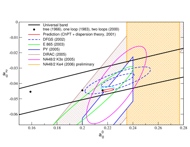
Figure 2: $S$ wave scattering lengths. Experimental results

The electromagnetic form factor is of particular interest in view of the Standard Model prediction for the magnetic moment of the muon. In this connection, the theoretical understanding of the final state interaction among the pions achieved in recent years can be used to reduce the experimental uncertainties, in particular in the region below 600 MeV, where the data are meager.[18] The $K$ to $\pi\pi$ transition form factors relevant for the third process allow a measurement of the phase difference between the $S$- and $P$-waves, $\delta_{0}^{0}-\delta_{1}^{1}$. The ellipse labeled E865[19] in figure 2 shows the constraint imposed on $a_{0}^{0}$ and $a_{0}^{2}$ by the $K_{e4}$ data collected at Brookhaven. The two ellipses denoted DFGS[20] represent the 1$\hskip 0.56917pt\sigma$ and 2$\hskip 0.56917pt\sigma$ contours obtained by combining these with other $\pi\pi$ data. The region labeled PY[21] has roughly the same experimental basis.

A very interesting proposal due to Cabibbo[22] has recently been explored in the NA48/2 experiment at CERN: the cusp seen near threshold in the decay $K^{\pm}\rightarrow\pi^{\pm}\pi^{0}\pi^{0}$ allows a measurement of the difference $a_{0}^{0}-a_{0}^{2}$ of scattering lengths.[23] In this case, the final state involves three pions, so that the analysis of the data is not a trivial matter.[24, 25, 26] As seen in the figure, the result is in good agreement with the Brookhaven data, as well as with the theoretical predictions. The same group has also investigated a very large sample of $K_{e4}$ decays.[27] The result for the scattering length $a_{0}^{0}$ is indicated by the broad vertical band. It is not in good agreement with E865, nor with their $K\rightarrow 3\pi$ result. The discrepancy calls for clarification.

An ideal laboratory for exploring the low energy properties of the pions is the atom consisting of a pair of charged pions, also referred to as pionium. The DIRAC collaboration at CERN has demonstrated that it is possible to generate such atoms and to measure their lifetime.[28] Since the physics of the bound state is well understood,[29] there is a sharp theoretical prediction for the lifetime.[1] The band labeled DIRAC in the figure shows that the observed lifetime confirms this prediction. Pionium level splittings would offer a clean and direct measurement of the second subtraction constant. Data on $\pi K$ atoms would also be very valuable, as they would allow to explore the role played by the strange quarks in the QCD vacuum.[29, 30]

5 Dispersion relations

After the above extensive discussion of our current knowledge of the two subtraction constants, I now wish to discuss their role in the low energy analysis of the $\pi\pi$ scattering amplitude, avoiding technical machinery as much as possible. Although the Roy equations represent an optimal and comprehensive framework for that analysis, the main points can be seen in a simpler context: forward dispersion relations.[31] More specifically, I consider the component of the scattering amplitude with $s$-channel isospin $I=0$, which I denote by $T^{0}(s,t)$. It satisfies a twice subtracted fixed-$t$ dispersion relation in the variable $s$. In the forward direction, $t=0$, this relation reads

$$\mbox{Re}\,T^{0}(s,0) = c_{0}+c_{1}\,s+\frac{s(s-4M_{\pi}^{2})}{\pi}\,P\int_{4M_{\pi}^{2}}^{\infty}\frac{dx\;\mbox{Im}\,T^{0}(x,0)}{x\,(x-4M_{\pi}^{2})\,(x-s)}+\rule{14.22636pt}{0.0pt}$$

$$+\,\frac{s(s-4M_{\pi}^{2})}{\pi}\int_{4M_{\pi}^{2}}^{\infty}\frac{dx\;\{\mbox{Im}\,T^{0}(x,0)-3\,\mbox{Im}\,T^{1}(x,0)+5\,\mbox{Im}\,T^{2}(x,0)\}}{3\,x\,(x-4M_{\pi}^{2})\,(x+s-4M_{\pi}^{2})}\,.$$

The symbol $P$ indicates that the principal value must be taken. The first integral accounts for the discontinuity across the right hand cut, while the second represents the analogous contribution from the left hand cut, where the components of the scattering amplitude with $I=1,2$ also show up. According to the optical theorem, the imaginary part of the forward scattering amplitude represents the total cross section: in the normalization of ACGL,[5] we have $\mbox{Im}\,T^{I}(s,0)=\sqrt{s(s-4M_{\pi}^{2})}\;\sigma^{I}_{tot}(s)$. In this notation, the physical total cross sections are given by

$$\sigma^{\pi^{\pm}\pi^{\pm}}_{tot} = \sigma^{2}_{tot}\,,\hskip 105.2751pt\sigma^{\pi^{\pm}\pi^{0}}_{tot}=\mbox{$\frac{1}{2}$}\sigma^{1}_{tot}+\mbox{$\frac{1}{2}$}\sigma^{2}_{tot}\,,\rule{28.45274pt}{0.0pt}$$ (6)

$$\sigma^{\pi^{\mp}\pi^{\pm}}_{tot} = \mbox{$\frac{1}{3}$}\sigma^{0}_{tot}+\mbox{$\frac{1}{2}$}\sigma^{1}_{tot}+\mbox{$\frac{1}{6}$}\sigma^{2}_{tot}\,,\hskip 31.2982pt\sigma^{\pi^{0}\pi^{0}}_{tot}=\mbox{$\frac{1}{3}$}\sigma^{0}_{tot}+\mbox{$\frac{2}{3}$}\sigma^{2}_{tot}\,.$$

As mentioned already, the subtraction term is determined by $a_{0}^{0},a_{0}^{2}$:

$$c_{0}+c_{1}\,s=32\,\pi\left\{a_{0}^{0}+(2a_{0}^{0}-5a_{0}^{2})\,\frac{s-4M_{\pi}^{2}}{12M_{\pi}^{2}}\right\}\,.$$ (7)

A dispersion relation of the above type also holds for other processes. What is special about $\pi\pi$ is that the contribution from the crossed channels can be expressed in terms of observable quantities – total cross sections in the case of forward scattering. The contribution from the left hand cut is dominated by the $\rho$-meson, which generates a pronounced peak in the total cross section with $I=1$. This contribution is known very accurately from the process $e^{+}e^{-}\rightarrow\pi^{+}\pi^{-}$. In the physical region, $s>4M_{\pi}^{2}$, the entire contribution from the crossed channels is a smooth function that varies only slowly with the energy. Note, however, that this contribution is by no means small.[32]

The angular momentum barrier suppresses the higher partial waves: at low energies, the first term in the partial wave decomposition

$$\mbox{Re}\,T^{0}(s,t) = 32\pi\left\{\mbox{Re}\,t^{0}_{0}(s)+5\,P_{2}(z)\,\mbox{Re}\,t^{0}_{2}(s)+\ldots\right\}$$ (8)

$$t = \mbox{$\frac{1}{2}$}(4M_{\pi}^{2}-s)(1-z)$$

represents the most important contribution. In the vicinity of the threshold, where the contribution from the higher angular momenta is negligibly small, the dispersion relation (5) thus amounts to an expression for the real part of the isoscalar $S$-wave. For brevity, I refer to this partial wave as $S^{0}$.

Equation (5) imposes a very strong constraint on $S^{0}$, for the following reason. Suppose that all partial waves except this one are known. The relation then determines Re$\,t^{0}_{0}(s)$ as an integral over Im$\,t^{0}_{0}(x)$. In the elastic region, unitarity already fixes the real part in terms of the imaginary part – we thus have two equations for the two unknowns Re$\,t^{0}_{0}(s)$ and Im$\,t^{0}_{0}(s)$. Accordingly, we may expect that, in the elastic region, the f.d.r. unambiguously fixes the $S^{0}$-wave. Indeed, this is borne out by the calculation, which is described in some detail elsewhere.[33]

One of the main results established in CGL is that the Roy equations fix the behaviour of the $S^{0}$-wave below 800 MeV almost entirely in terms of three parameters: the two subtraction constants $a_{0}^{0},a_{0}^{2}$ and the value of the phase at 800 MeV. In particular, the behaviour of the scattering amplitude at high energies is not important. This can also be seen on the basis of equation (5): replacing our representation of the scattering amplitude above $K\bar{K}$ threshold by the one proposed in KPY,[31] for instance, the solution of the f.d.r. very closely follows the solution of the Roy equations that belongs to the same value of the phase at 800 MeV.[33]

6 The lowest resonances of QCD

The positions of the poles in the S-matrix represent universal properties of the strong interaction, which are unambiguous even if the width of the corresponding resonance turns out to be large,[34] but they concern the non-perturbative domain, where an analysis in terms of the local degrees of freedom of QCD – quarks and gluons – is not in sight. First quenched lattice explorations of the pole from the $\sigma$ have appeared,[35] but in view of the strong final state interaction in this channel, it will take some time before this state can reliably be reached on the lattice.

One of the reasons why the values for the pole position of the $\sigma$ quoted by the Particle Data Group cover a very broad range is that all of these rely on the extrapolation of hand made parametrizations: the data are represented in terms of suitable functions on the real axis and the position of the pole is determined by continuing this representation into the complex plane. If the width of the resonance is small, the ambiguities inherent in the choice of the parametrization do not significantly affect the result, but the width of the $\sigma$ is not small.

A popular approach to the problem is based on the so-called inverse amplitude method. Applying it to the $\chi$PT representation of the scattering amplitude[36] invariably produces a pole in the right ball park. The procedure definitely improves the quality of the two-loop approximation of $\chi$PT on the real axis, because it respects unitarity in the elastic region. The extrapolation into the complex plane, however, also contains a number of fake singularities. Like all other parametrizations, this approach relies on a model. I do not know of a way to estimate the systematic uncertainties generated if QCD is replaced by one model or the other – if error estimates are given at all, these necessarily rely on guesswork. A thorough discussion of the problems inherent in the IAM approach appeared several years ago.[37]

We have found a method that does not require a parametrization of the data at all. It relies on the fact that (a) the $S$-matrix has a pole on the second sheet if and only if it has a zero on the first sheet, (b) the Roy equations are valid not only on the real axis, but in a limited domain of the first sheet, (c) the poles from the lowest resonances, $\sigma$, $\rho$, $f_{0}(980)$, all occur in that domain. The numerical evaluation of the pole position is straightforward. The one closest to the origin occurs at[2]

$$M_{\sigma}-\frac{i}{2}\,\Gamma_{\sigma}=\sqrt{s_{\sigma}}=441\,\rule[-1.99997pt]{0.0pt}{10.00002pt}^{+16}_{-\,8}-\,i\;272\,\rule[-1.99997pt]{0.0pt}{10.00002pt}^{+\,9}_{-12.5}\;\mbox{MeV}\,,$$ (9)

where the error accounts for all sources of uncertainty. We may, for instance, replace our representation for $S^{0}$ by the one proposed by Bugg[38] or replace the entire scattering amplitude by the parametrization in KPY.[31] In either case, the outcome for the pole position is in the above range. For more details, I refer to CCL[2] and to a recent conference report.[39]

In the meantime, the method described above was applied to the case of $\pi K$ scattering, with the result that the lowest resonance in that channel occurs at $m_{\kappa}=(658\pm 13)-i\,(278.5\pm 12)$ MeV.[40] Evidently, the physics of the $\kappa$ is very similar to the one of the $\sigma$.

7 On the working bench

We are currently extending the work described in CGL to higher energies. The price to pay is that the contributions from the high energy region then become more important. Since the first few terms of the partial wave expansion do not represent a decent approximation there, one instead uses a Regge representation for the asymptotic domain. In CGL, we borrowed that from Pennington.[41] In the meantime, we have performed a new Regge analysis, invoking experimental information as well as sum rules to pin down the residue functions.

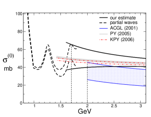
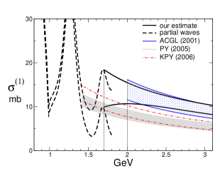
Figure 3: Asymptotic behaviour of the total cross sections with $I_{t}=0$ and $I_{t}=1$.

Brief accounts of this work were given elsewhere.[42] Figure 3 shows the preliminary results obtained for the total cross sections with $t$-channel isospin 0 and 1:

$$\sigma_{tot}^{(0)}=\mbox{$\frac{1}{3}$}\sigma_{tot}^{0}+\sigma_{tot}^{1}+\mbox{$\frac{5}{3}$}\sigma^{2}_{tot}\,,\hskip 5.69046pt\sigma_{tot}^{(1)}=\mbox{$\frac{1}{3}$}\sigma_{tot}^{0}+\mbox{$\frac{1}{2}$}\sigma_{tot}^{1}-\mbox{$\frac{5}{6}$}\sigma^{2}_{tot}\,.$$ (10)

We include pre-asymptotic contributions and assume that the Regge parametrization yields a decent approximation above 1.7 GeV. At lower energies, the uncertainties in that representation become larger than those in the sum over the partial waves, which is also shown. The comparison with the representation used in ACGL confirms the cross section with $I_{t}=1$, while the one for $I_{t}=0$ comes out larger by 1 or $2\hskip 1.42271pt\sigma$. In the solutions of the Roy equations, the effects generated by such a shift are barely visible below 800 MeV. We hope to complete the analysis soon, as well as the application to the electromagnetic form factor of the pion, for which an accurate representation is needed in connection with the Standard Model prediction for the magnetic moment of the muon.

It is a pleasure to thank the organizers of the meeting for their kind hospitality during a very pleasant stay at Chapel Hill and Claude Bernard, Leonardo Giusti and Steve Sharpe for useful comments about the text. Also, I acknowledge Balasubramanian Ananthanarayan, Irinel Caprini, Gilberto Colangelo and Jürg Gasser for a most enjoyable and fruitful collaboration – the present report is based on our common work.

References

- [1] G. Colangelo, J. Gasser and H. Leutwyler, Nucl. Phys. B 603 (2001) 125.
- [2] I. Caprini, G. Colangelo and H. Leutwyler, Phys. Rev. Lett. 96 (2006) 132001.
- [3] W.-M. Yao et al. [Particle Data Group], Journal of Physics G 33 (2006) 1.
- [4] S. M. Roy, Phys. Lett. B 36 (1971) 353.
- [5] B. Ananthanarayan, G. Colangelo, J. Gasser and H. Leutwyler, Phys. Rept. 353 (2001) 207.
- [6] J. L. Basdevant, C. D. Froggatt and J. L. Petersen, Nucl. Phys. B 72 (1974) 413.
- [7] V. Bernard and U. G. Meissner, hep-ph/0611231, give an excellent overview of recent developments in PT , with many references to ongoing work.
- [8] S. Weinberg, Phys. Rev. Lett. 17 (1966) 616.
- [9] J. Gasser and H. Leutwyler, Phys. Lett. B 125 (1983) 325; Annals Phys. 158 (1984) 142.
- [10] J. Bijnens, G. Colangelo, G. Ecker, J. Gasser and M. E. Sainio, Phys. Lett. B 374 (1996) 210; Nucl. Phys. B 508 (1997) 263; ibid. B 517 (1998) 639 (E).
- [11] For a detailed discussion of the scalar form factor and references to related work, see B. Ananthanarayan et al., Phys. Lett. B602, 218 (2004).
- [12] C. Aubin et al., [MILC Collaboration], Phys. Rev. D 70 (2004) 114501.
- [13] J. Gasser and H. Leutwyler, Nucl. Phys. B 250 (1985) 465, section 11.
- [14] L. Del Debbio, L. Giusti, M. Lüscher, R. Petronzio and N. Tantalo, hep-lat/0610059.
- [15] G. Colangelo, J. Gasser and H. Leutwyler, Phys. Rev. Lett. 86 (2001) 5008.
- [16] I thank Karl Jansen and Andrea Shindler for this information. The method used is described in K. Jansen and C. Urbach [ETM Collaboration], hep-lat/0610015; A. Shindler [ETM Collaboration], hep-ph/0611264.
- [17] S. R. Beane, P. F. Bedaque, K. Orginos and M. J. Savage [NPLQCD Collaboration], Phys. Rev. D 73 (2006) 054503.
- [18] G. Colangelo, AIP Conf. Proc. 756 (2005) 60.
- [19] S. Pislak et al. [BNL-E865 Collaboration], Phys. Rev. Lett. 87 (2001) 221801; Phys. Rev. D 67 (2003) 072004.
- [20] S. Descotes-Genon, N. H. Fuchs, L. Girlanda and J. Stern, Eur. Phys. J. C 24 (2002) 469.
- [21] J. R. Pelaez and F. J. Yndurain, Phys. Rev. D 71 (2005) 074016.
- [22] N. Cabibbo, Phys. Rev. Lett. 93 (2004) 121801.
- [23] J. R. Batley et al. [NA48/2 Collaboration], Phys. Lett. B 633, 173 (2006).
- [24] N. Cabibbo and G. Isidori, JHEP 0503 (2005) 021.
- [25] G. Colangelo, J. Gasser, B. Kubis and A. Rusetsky, Phys. Lett. B 638 (2006) 187.
- [26] E. Gamiz, J. Prades and I. Scimemi, hep-ph/0602023.
- [27] L. Masetti, Proc. ICHEP06, hep-ex/0610071.
- [28] B. Adeva et al. [DIRAC Collaboration], Phys. Lett. B 619 (2005) 50.
- [29] A thorough review is contained in Proc. Workshop on Hadronic Atoms 2005, eds. L. Afanasyev, G. Colangelo and J. Schacher, hep-ph/0508193.
- [30] J. Schweizer, Eur. Phys. J. C 36 (2004) 483; Phys. Lett. B 587 (2004) 33.
- [31] R. Kaminski, J. R. Pelaez and F. J. Yndurain, Phys. Rev. D 74 (2006) 014001 [Erratum-ibid. D 74 (2006) 079903].
- [32] The significance of the contributions from the left hand cut is thoroughly discussed in Z. Y. Zhou, G. Y. Qin, P. Zhang, Z. G. Xiao, H. Q. Zheng and N. Wu, JHEP 0502 (2005) 043.
- [33] H. Leutwyler, in Proc. Quark Confinement and the Hadron Spectrum VII, Ponta Delgada, Azores islands, Portugal (2006), hep-ph/0612111.
- [34] See for example R.J. Eden, P.V. Landshoff, D.I. Olive, J.C. Polkinghorne, The analytic S-matrix, Cambridge University Press (1966) or D. Zwanziger, Phys. Rev. 131 (1963) 888.
- [35] H. Y. Cheng, C. K. Chua and K. F. Liu, Phys. Rev. D 74 (2006) 094005.
- [36] T. N. Truong, Phys. Rev. Lett. 61, 2526 (1988); A. Dobado, M. J. Herrero and T. N. Truong, Phys. Lett. B 235, 134 (1990); A. Dobado and J. R. Pelaez Phys. Rev. D 56 (1997) 3057; J. A. Oller, E. Oset and J. R. Pelaez, Phys. Rev. D 59 (1999) 074001, D 60 (1999) 099906 (E); T. Hannah, Phys. Rev. D 60 (1999) 017502.
- [37] G. Y. Qin, W. Z. Deng, Z. G. Xiao and H. Q. Zheng, Phys. Lett. B 542 (2002) 89.
- [38] D. V. Bugg, hep-ph/0608081.
- [39] H. Leutwyler, in Proc. MESON 2006, Krakow, Poland, hep-ph/0608218.
- [40] S. Descotes-Genon and B. Moussallam, arXiv:hep-ph/0607133.
- [41] M. R. Pennington, Annals Phys. 92 (1975) 164.
- [42] I. Caprini, in these proceedings; I. Caprini, G. Colangelo and H. Leutwyler, Int. J. Mod. Phys. A 21 (2006) 954.