Effect of charged partons on black hole production at the Large Hadron Collider

Abstract:

The cross section for black hole production in hadron colliders is calculated using a factorization hypothesis in which the parton-level process is integrated over the parton density functions of the protons. The mass, spin, charge, colour, and finite size of the partons are usually ignored. We examine the effects of parton electric charge on black hole production using the trapped-surface approach of general relativity. Accounting for electric charge of the partons could reduce the black hole cross section by one to four orders of magnitude at the Large Hadron Collider. The cross section results are sensitive to the Standard Model brane thickness. Lower limits on the amount of energy trapped behind the event horizon in the collision of charged particles are also calculated.

1 Introduction

Models of large [1, 2, 3] or warped [4, 5] extra dimensions allow the fundamental scale of gravity to be as low as the electroweak scale. For energies above the gravity scale, black holes can be produced in particle collisions. This opens up the possibility to produce black holes at the Large Hadron Collider (LHC). Once formed, the black hole will decay by emitting Hawking radiation [6]. The final fate of the black hole is unknown since quantum gravity will become important as the black hole mass approaches the Planck scale. If black holes are produced at the LHC, detecting them will not only test general relativity and probe extra dimensions, but will also teach us about quantum gravity.

Early discussions of black hole production in colliders postulated a $\pi r_{\mathrm{h}}^{2}$ form for the cross section, where $r_{\mathrm{h}}$ is the horizon radius of the black hole formed in the parton scattering process [7, 8, 9]. Calculations based on classical general relativity have had limited success in improving the cross section estimates [10, 11]. The effects of mass, spin, charge, colour, and finite size of the incoming particles are usually neglected in these calculations. The effects of finite size have been examined [12, 13] and only recently have angular momentum [14] or charge been discussed [15]. Although these results are far from complete, they do indicated that the simple geometric cross section is correct if multiplied by a formation factor of order unity [16].

General relativistic calculations of the cross section have usually been performed using the trapped-surface approach. The two incoming partons are modeled as Aichelburg-Sexl shock waves [17]. Spacetime is flat in all regions of space except at the shocks. The union of these shock waves defines a closed trapped surface. Black hole formation can be predicted by identifying a future trapped surface, with no need to calculate the gravitational field.

The trapped-surface approach was first applied to TeV-scale gravity calculations by Eardley and Giddings [10] in four dimensions. Thier work was extended to the $D$-dimensional case numerically by Yoshino and Nambu [11]. The numerical studies were improved by Yoshino and Rychkov [14] by analyzing the closed trapped surface on a different slice of spacetime. These general relativistic calculations have enabled lower limits to be obtained for the black hole production cross section of colliding particles in TeV-scale gravity scenarios.

Since black holes are highly massive objects, the momentum fraction of the partons in the protons that form them must be high. Thus typically valence quarks will be involved in black hole formation. This means the most probable charge of the black hole in proton collisions will be $+4/3$. Since the gravitational field of each particle is determined by its energy-momentum tensor, charge should affect the black hole formation. First exploratory work by Yoshino and Mann [15] obtained a condition on the electric charges of the colliding particles for a closed trapped surface to form. The results depend on the Standard Model brane thickness. Since the LHC is about to start up, it is useful to investigate ideas, such as these, that modify black hole production.

In this paper, we use the Yoshino and Mann charge condition in its general form and build on their work by examining the effect of charge on black hole production at the LHC. The cross section is obtained by summing over all possible parton pairs in the protons. By using the parton density functions of the proton and applying the charge condition, we obtain the black hole cross section. The amount of available energy that goes into the black hole formation is also examined.

An outline of this paper is as follows. We first review the trapped-surface approach in section 2. Then in section 3, we examine the Reissner-Nordström spacetime of charged particles in higher dimensions. Following Yoshino and Mann [15], we obtain the condition for an apparent horizon in section 4. Since electric charge is confined to the three-brane, we relate the higher-dimensional charge in the Reissner-Nordström metric to the Standard Model electric charge as the second step in our approach. We then translate the condition for apparent horizon formation into a condition for charged partons to form a black hole at the LHC. Lower limits on the amount of energy trapped behind the apparent horizon are shown in section 5. In section 6, we apply the charge condition to the calculation of the black hole cross section for different values of the Planck scale, number of dimensions, and Standard Model brane thickness. We conclude with a discussion in section 7.

2 Trapped surfaces and apparent horizon

In this section, we review the concepts of Aichelburg-Sexl shock waves, trapped surfaces, and the apparent horizon. A charged particle can be modelled using the Reissner-Nortsröm metric. By boosting the Reissner-Nortström spacetime and taking the lightlike limit, we obtain an approximation of a charged ultrarelativistic particle. The gravitational field of the point massless particle is thus infinitely Lorentz contracted and forms a longitudinal plane-fronted Aichelburg-Sexl gravitational shock wave. Except at the shock wave, spacetime is flat before the collision. By combining two Aichelburg-Sexl shock waves, we set up a head-on collision of ultrelativistic particles. At the instance of collision, the two shock waves pass through one another, and interact nonlinearly by shearing and focusing. After the collision, the two shocks continue to interact nonlinearly with each other and spacetime within the future lightcone of the collision becomes highly curved.

To describe this nontrivial collision process, we choose the lightcone coordinates $u=t-z$ and $v=t+z$. Four regions of spacetime can be identified.

Region I:

$u<0,v<0$, before the collision,

Region  II:

$u>0,v<0$, after the wave at $u=0$ has passed,

Region III:

$v>0,u<0$, after the wave at $v=0$ has passed,

Region IV:

$u>0,v>0$, interaction region after the waves have passed.

Except at the shock waves, spacetime is flat in regions I, II, and III before the collision. No one has been able to calculate the metric in the future of the collision (non-linear region IV) except perturbatively in the distance far from the interaction $u=v=0$ [18, 19, 20]. It is possible to investigate the collision on the slice $u\leq 0,v=0$ and $v\leq 0,u=0$. It is also possible to proceed with the analysis on the slice of the future lightcone of the shock collision plane, given by the union of the outgoing shocks $u=0,v\geq 0$ and $v=0,u\geq 0$. This is the future most slice that can be used without knowledge of region IV.

The different regions of spacetime can be examined for trapped surfaces. We search for marginally trapped-surface formation on a slice of spacetime $u=0$, $v\geq 0$ and $v=0$, $u\geq 0$. A marginally trapped surface is define as a closed spacelike ($D-2$)-surface, the outer null normals of which have zero convergence [21]. Moving a small distance inside the marginally trapped surface one can find a true closed trapped surface with negative convergence. In physical terms this means that there is a closed surface whose normal null geodesics do not diverge, and so are trapped by gravity. For a Schwarzschild black hole, the marginally trapped surface is a sphere around the singularity, which happens to coincide with the event horizon [22].

An apparent horizon is the outermost marginally trapped surface. The existence of a marginally trapped surface means either that the marginally trapped surface is the apparent horizon, or that an apparent horizon exits in the exterior of the marginally trapped surface. Existence of an apparent horizon implies the presence of a singularity in the future. Assuming cosmic censorship [23], this singularity must be hidden behind an event horizon, and we may conclude that a black hole will form. Moreover, the black hole horizon must lie outside the closed trapped surface. Formation of the apparent horizon is then a sufficient condition for formation of a black hole for which the event horizon is outside the apparent horizon [24]. Thus if one can prove the existence of a trapped surface, then one knows that in the future the solution will involve a black hole.

The area of a marginally trapped surface is a lower bound on the area of the apparent horizon. Using this information, one can estimate the event horizon area and, via the area theorem [25], the mass of the formed black hole. Since the black hole horizon is always in the exterior region, the trapped surface method gives only a lower bound on the final black hole mass. The black hole mass can have any value between this bound and the centre of mass energy of the collision.

3 $D$-Dimensional Reissner-Nordström spacetime

The Reissner-Nordström solution describing the gravitation field of a point particle of mass $m$ and electric charge $q$ in $D$ dimensions in spherical coordinates ($T,R,\Phi_{1},\ldots,\Phi_{D-2}$) is

$$ds^{2}=-g(R)dT+g(R)^{-1}dR^{2}+R^{2}d\Omega^{2}_{D-2}\,,$$ (1)

where

$$g(R) = 1-\frac{2M}{R^{D-3}}+\frac{Q^{2}}{R^{2(D-3)}}\,,$$ (2)

$$M = \frac{8\pi G_{D}m}{(D-2)\Omega_{D-2}}\,,$$ (3)

$$Q^{2} = \frac{8\pi G_{D}q^{2}}{(D-2)(D-3)}\,,$$ (4)

$G_{D}$ is the $D$-dimensional gravitational constant, and $d\Omega_{D-2}$ and $\Omega_{D-2}$ are the line element and volume of a ($D-2$)-dimensional unit sphere, given by

$$\Omega_{D-2}=\frac{2\pi^{(D-1)/2}}{\Gamma[(D-1)/2]}\,,$$ (5)

where $\Gamma$ is Euler’s Gamma function. The energy-momentum tensor used in Einstein’s equation is that of the electromagnetic field in the spacetime that results from the charge on the particle. The metric is a unique spherically symmetric asymptotically flat solution of the Einstein-Maxwell equations and is locally similar to the Schwarzschild solution. The Reissner-Nordström solution does not describe the spin, magnetic moment, or colour charge of a particle.

The condition for the existence of an event horizon in $D$-dimensional Reissner-Nordström spacetime ($Q^{2}\leq M^{2}$) is

$$|q|\leq\frac{m}{\Omega_{D-2}}\sqrt{\frac{8\pi G_{D}(D-3)}{D-2}}\,.$$ (6)

We will return to this condition after we have related the electric charge in higher-dimensional Maxwell theory to the electric charge in four dimensions. For the moment, we are ignoring that the electric charge of the particle is confined to the Standard Model three-brane. We will consider the black hole production process as happening in flat $D$-dimensional spacetime since the horizon radius is much small than the compactification radius.

Before Lorentz boosting the Reissner-Nordström metric, it is convenient to convert the metric to isotropic coordinates ($\bar{T},\bar{Z},\bar{R},\bar{\Phi}_{1},\ldots,\bar{\Phi}_{D-3}$), where $\bar{T}=T$, $\bar{Z}=Z$, $\bar{R}=\sqrt{\bar{Z}^{2}+\bar{r}^{2}}$, $R^{2}d\Omega_{D-2}^{2}=d\bar{Z}^{2}+d\bar{r}^{2}+\bar{r}^{2}d\bar{\Omega}_{D-3}^{2}$, and

$$R=\bar{R}\left(1+\frac{M}{\bar{R}^{D-3}}+\frac{M^{2}-Q^{2}}{4\bar{R}^{2(D-3)}}\right)^{\frac{1}{D-3}}.$$ (7)

When the Reissner-Nordström metric is boosted, the rest mass $m$ and charge $q$ are fixed and boosted to a finite value of $\gamma$. In the ultrarelativistic limit ($\gamma\to\infty$) both terms in eq. (2) diverge unless we take both $m$ and $q$ to vanish in this limit. Thus, we boost the Reissner-Nordström solution by taking the limit of large boost and small $m$ with fixed total energy

$$E=\gamma m\,,$$ (8)

and small $q^{2}$ with fixed quantity

$$p_{e}^{2}=\gamma q^{2}\,.$$ (9)

This is consistent with the lightlike limit of a particle with mass and electric charge. Choosing the particle to move in the $+Z$ direction in $D$-dimensional spacetime, the boosted coordinates are ($t,z,r,\phi_{1},\ldots,\phi_{D-3}$), where $\bar{T}=\gamma(t-\beta z)$, $\bar{Z}=\gamma(z-\beta t)$, $r=\bar{R}$, and $\phi_{i}=\bar{\Phi}_{i}$. After the transformation, we take the lightlike limit.

Next we define the retarded and advanced times ($\bar{u}=t-z$ and $\bar{v}=t+z$, also $\bar{r}=r$ and $\bar{\phi}_{i}=\phi_{i}$) to obtain the coordinates ($\bar{u},\bar{v},\bar{r},\bar{\phi}_{1},\ldots,\bar{\phi}_{D-3}$). This yields a finite result that is the charged version of the $D$-dimensional Achelburg-Sexl metric [15, 26, 27]:

$$ds^{2}=-d\bar{u}d\bar{v}+d\bar{r}^{2}+\bar{r}^{2}d\bar{\Omega}_{D-3}+\Phi(\bar{r})\delta(\bar{u})d\bar{u}^{2}\,,$$ (10)

where

$$\Phi(\bar{r})=\left\{\begin{array}[]{ll}-8G_{D}E\ln\bar{r}-\frac{2a}{\bar{r}}&(D=4)\,,\\ \frac{16\pi G_{D}E}{(D-4)\Omega_{D-3}\bar{r}^{D-4}}-\frac{2a}{(2D-7)\bar{r}^{2D-7}}&(D\geq 5)\,,\end{array}\right.$$

and

$$a=\frac{2\pi(4\pi G_{D}p_{e}^{2})}{D-3}\frac{(2D-5)!!}{(2D-4)!!}\,.$$ (11)

The charge dependence is entirely contained in the general charge parameter $a$. The function $\Phi$ depends only on the transverse radius $\bar{r}=\sqrt{\bar{x}^{i}\bar{x}_{i}}$. The Aichelburg-Sexl metric is a solution for a point particle (delta function source) moving at the speed of light. The metric eq. (10)-(11) reduces to the usual Aichelbrg-Sexl metric in the limit $q\to 0$. For the particles we will consider in this study, $\gamma\gtrsim 5\times 10^{3}$ and the mean value of $\gamma$ is about $7\times 10^{5}$. The charged version of the Aichelberg-Sexl metric is thus a good approximation to an ultrarelativistic massive charged particle with finite, but large, $\gamma$.

The delta function in eq. (10) indicates that the $(\bar{u},\bar{v},\bar{r},\bar{\phi}_{i})$ coordinates are discontinuous at $\bar{u}=0$. These coordinates are unsuitable for analysing the behaviour of geodesics crossing the shock at $\bar{u}<0$, which is necessary for understanding the causal structure. In the following, we define

$$r_{0}=\left(\frac{8\pi G_{D}E}{\Omega_{D-3}}\right)^{\frac{1}{D-3}}\equiv 1$$ (12)

as the unit of length. We introduce new coordinates ($u,v,r,\phi_{i}$), which are continuous and smooth across the shock using the transformations

$$\bar{u} = u\,,$$ (13)

$$\bar{v} = v+F(u,r)\,,$$ (14)

$$\bar{r} = G(u,r)\,,$$ (15)

$$\bar{\phi}_{i} = \phi_{i}\,,$$ (16)

where $F(u,r)=0$ and $G(u,r)=r$ for $u<0$. In these coordinates, we require $v$, $r$, and $\phi_{i}$ equal a constant to be a null geodesic with affine parameter $u$. The metric in these coordinates becomes

$$ds^{2}=-dudv+G_{,r}^{2}dr^{2}+G^{2}d\Omega_{D-3}^{2}\,,$$ (17)

where $G$ and $G_{,r}$ are explicitly given by [15]

$$G = r+\frac{u\theta(u)}{r^{D-3}}\left(1-\frac{a}{r^{D-3}}\right),$$ (18)

$$G_{,r} = 1+(D-3)\frac{u\theta(u)}{r^{D-2}}\left(1-\frac{2a}{r^{D-3}}\right),$$ (19)

where $\theta(u)$ is the Heaviside step function. Both geodesics and their tangents are now continuous across the shock, and two coordinate singularities appear in the region $u>0$. These singularities have been analyzed in Ref. [15].

4 Condition for apparent horizon formation

To setup the two-particle head-on collision, we consider a second identical shock wave traveling along $\bar{v}=0$ in the $-Z$ direction. By causality, the two shock waves will not be able to influence each other until the shocks collide. This means that we can superimpose two of the above solutions to give the exact geometry outside the future lightcone of the collision of the two shocks. We assume without loss of generality that the two particles have the same energy $E$ but different charge parameters $p_{e}^{(1)}$ and $p_{e}^{(2)}$.

In the remainder of this section, we follow Yoshino and Mann [15] directly in studying the apparent horizon on the slice $u>0$, $v=0$ and $v>0$, $u=0$. The closed trapped surfaces are symmetric under rotation of the transverse directions and the reflection $z\to-z$. Because the system is axisymmetric, the location on the apparent horizon surface on each side of $z$ is given by a function of $r$. We assume the apparent horizon is given by the union of two surfaces $S_{1}$ and $S_{2}$, where

$$S_{1}:u=h^{(1)}(r) (r_{\mathrm{min}}\leq r\leq r_{\mathrm{max}}^{(1)})\quad\mathrm{on}\quad u\geq 0\ \mathrm{and}\ v=0,$$ (20)

$$S_{2}:v=h^{(2)}(r) (r_{\mathrm{min}}\leq r\leq r_{\mathrm{max}}^{(2)})\quad\mathrm{on}\quad v\geq 0\ \mathrm{and}\ u=0,$$ (21)

where $h^{(1)}$ and $h^{(2)}$ are monotonically increasing functions of $r$. When $S_{1}$ and $S_{2}$ cross $u=v=0$, $r=r_{\mathrm{min}}$. Continuity of the metric at the apparent horizon requires $S_{1}$ and $S_{2}$ to coincide with each other at $u=v=0$. At $r_{\mathrm{max}}^{(1)}$ and $r_{\mathrm{max}}^{(2)}$, we require $h^{(1)}(r)$ and $h^{(2)}(r)$ to cross the coordinate singularity. The surface becomes a closed trapped surface by the above arguments.

Following Yoshino and Mann [15], one derives the equations for $h^{(1)}(r)$ and $h^{(2)}(r)$, and the differential equation for the apparent horizon is then obtained. The boundary condition that must be imposed at $r=r_{\mathrm{min}}$ is

$$h_{,r}^{(1)}(r_{\mathrm{min}})h_{,r}^{(2)}(r_{\mathrm{min}})=4\,,$$ (22)

where both $h_{,r}^{(1)}(r_{\mathrm{min}})$ and $h_{,r}^{(2)}(r_{\mathrm{min}})$ are positive. Using this boundary condition, the apparent horizon equation is solved and the boundary condition become

$$x^{4}=(x-a_{1})(x-a_{2})\,,$$ (23)

where $x\equiv r_{\mathrm{min}}^{D-3}$. This equation determines the value of $r_{\mathrm{min}}$. The apparent horizon exists if, and only if, there is a solution to eq. (23) with $x>a_{1}$ and $x>a_{2}$.

4.1 Condition on general charges

The special cases of collisions of particles with the same charge, and collisions of a charged and a neutral particle have been previously examined [15]. We examine the case of general charge parameters and note the simplifying cases.

Equation (23) has four roots. For $a_{1}>0$ and $a_{2}>0$ two solutions will have $x<a_{1}$ and $x<a_{2}$, and not correspond to an apparent horizon. We investigate the other two solutions. Figure 1 shows two representative cases of eq. (23). We see that an apparent horizon exists if, and only if, the local minimum in the $x>0$ region is less than or equal to zero. The location of the minium is given by differentiating the quartic equation, eq. (23), and solving the resulting cubic equation for the positive root. The solution is

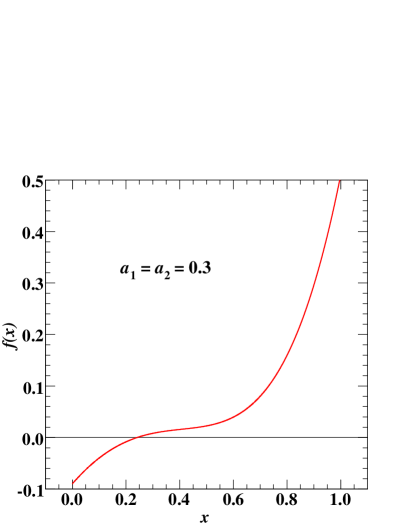
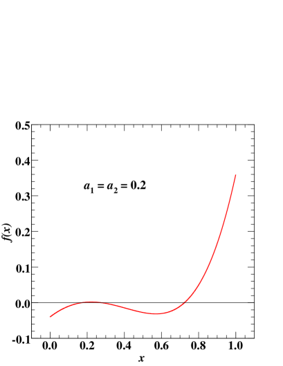
Figure 1: Representative cases for the quartic equation $f(x)=x^{4}-(x-a_{1})(x-a_{2})$.

$$x=\sqrt{\frac{2}{3}}\cos\left(\frac{\pi-\theta}{3}\right)\,,$$ (24)

where

$$\tan\theta=\sqrt{\left(\frac{2}{3}\right)^{3}\frac{1}{(a_{1}+a_{2})^{2}}-1}\,.$$ (25)

Substituting this value into eq. (23) and drawing the contour, we find the region for apparent horizon formation in the $(a_{1},a_{2})$-plane, as shown in fig. 2. We see that both $a_{1}$ and $a_{2}$ must be sufficiently small for apparent horizon formation. For two particles of equal charge: $a_{1}=a_{2}=1/4$ gives $x=1/2$, which is a solution of eq. (23). For one charged particle and one neutral particle: $a_{1}=a=2/(3\sqrt{3})$ and $a_{2}=0$ gives $x=1/\sqrt{3}$, which is also a solution of eq. (23).

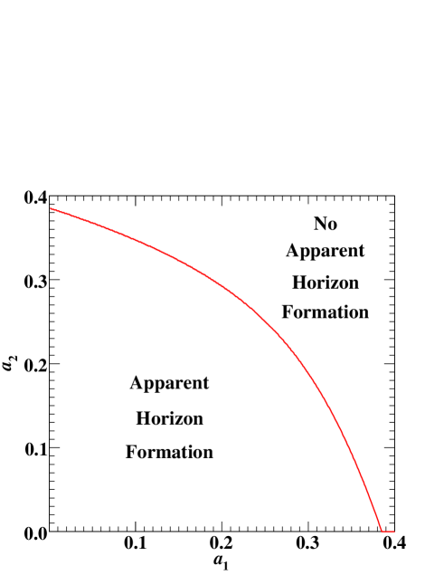
Figure 2: Region of the apparent horizon formation in the $(a_{1},a_{2})$-plane.

We can understand the requirement on $a_{1}$ and $a_{2}$ physically as follows. Since $a_{1}$ and $a_{2}$ are proportional to $(p_{e}^{(1)})^{2}$ and $(p_{e}^{(2)})^{2}$, the condition derived in eq. (23) does not depend on the sign of the charge of either particle. This is because the gravitational field due to each charge is generated by an electromagnetic energy-momentum tensor $T_{\mu\nu}^{(\mathrm{em})}\sim p_{e}^{2}\delta(\bar{u})/\bar{r}^{2D-5}$ that depends on the square of the charge. The gravitational field induced by $T_{\mu\nu}^{(\mathrm{em})}$ of the incoming particles is repulsive, and its affect becomes dominant around the centre. As the value of $a$ increases, the repulsive region becomes larger, preventing formation of the apparent horizon. The critical value of $a$ for apparent horizon formation occurs when the repulsive gravitational force due to the electric field becomes equivalent to the self-attractive force due to the energy of the system.

4.2 Condition on parton electric charges

The approach for handling the confinement of the electric field to the Standard Model three-brane is far from clear. So far, we have ignored this effect by using the $D$–dimensional Einstein-Maxwell theory. Assuming the boosted Reissner-Nordström metric represents the gravitational field of an elementary particle with electric charge moving at high speed, we develop the relationship between the electric charge in four dimensions $q_{4}$ and the charge in higher-dimensional Maxwell theory $q$. For two particles in $D$ dimensions with the same charge at rest, for example, the force between them is

$$F=\frac{q^{2}}{r^{D-2}}\,.$$ (26)

Since we have been using Gaussian units, the factor of $1/\Omega_{D-2}$ ($1/4\pi$ in the case of four dimensions) is absorbed into the definition of the charge. If the gauge fields are confined to the Standard Model brane, the only characteristic length scale is the width of the brane, which should be of the order of the Planck length. We introduce the constant $C_{\mathrm{brane}}$:

$$\frac{1}{M_{D}}\to\frac{C_{\mathrm{brane}}}{M_{D}}\,,$$ (27)

where $C_{\mathrm{brane}}$ is a dimensionless quantity of order unity. For sufficiently large $r$,

$$F\to\frac{q^{2}}{r^{2}}\left(\frac{M_{D}}{C_{\mathrm{brane}}}\right)^{D-4}=\frac{q_{4}^{2}}{r^{2}}\,.$$ (28)

This condition is reasonable since the Compton wavelength $1/M_{D}$ of the black hole is much smaller than its horizon radius $r_{\mathrm{h}}$. Thus

$$q^{2}=q_{4}^{2}\left(\frac{C_{\mathrm{brane}}}{M_{D}}\right)^{D-4}\,.$$ (29)

The brane thickness is a measure of how confined the Standard Model electric charge is to the brane. If the brane is thick, the Maxwell theory would be higher dimensional in the neighbourhood of the particle. We let

$$q_{4}^{2}=C_{q}^{2}\alpha\,,$$ (30)

where $C_{q}$ is the charge in units of elementary charge $e$ ($-1/3$ or $+2/3$ for quarks and 0 for gluons) and $\alpha$ is the fine structure constant. Our treatment of the electric charge has not fully taken into account the effects of confinement of the electric field on the brane. We have also ignored the brane tension and the structure of the extra dimensions.

Using eq. (29), eq. (30),

$$G_{D}^{-1}=\frac{8\pi}{(2\pi)^{D-4}}M_{D}^{D-2}\,,$$ (31)

and recalling the definition of the volume of the ($D-2$)-dimensional unit sphere given by eq. (5), we obtain for eq. (11)

$$\frac{a}{r_{0}^{2(D-3)}}=C_{q}^{2}\alpha\left(\frac{M_{D}}{m}\right)\left(\frac{M_{D}}{E}\right)\pi\frac{\Omega_{D-3}^{2}}{D-3}\frac{(2D-5)!!}{(2D-4)!!}\left(\frac{C_{\mathrm{brane}}}{2\pi}\right)^{D-4}\,,$$ (32)

where we have reintroduced the unit length $r_{0}$. Choosing values for $\alpha$ and $m$, we can use eq. (32) to study the condition for apparent horizon formation as a function of $D$, $M_{D}$, and $C_{\mathrm{brane}}$. An apparent horizon will not occur at the instance of collision if the brane is thick or if the spacetime dimensionality is low. Charge effects will not be significant at high energies.

5 Trapped energy

We now consider how much energy is trapped behind the horizon in black hole formation from charged-particle collisions. From section 2, we saw that the event horizon must be outside the apparent horizon. The area theorem [25] states that the event horizon area can never decreases. Hence, we naturally expect the apparent horizon mass to be defined by

$$M_{\mathrm{AH}}=\frac{(D-2)\Omega_{D-2}}{16\pi G_{D}}\left(\frac{A_{D-2}}{\Omega_{D-2}}\right)^{\frac{D-3}{D-2}}\,,$$ (33)

where $A_{D-2}$ is the ($D-2$)-dimensional area of the apparent horizon give by

$$A_{D-2}=\frac{2}{D-2}\Omega_{D-3}r_{0}^{D-2}x^{\frac{D-2}{D-3}}\,.$$ (34)

This mass provides a lower bound on the mass of the final black hole, and thus $M_{\mathrm{AH}}$ is an indicator of the energy trapped behind the event horizon. The parameter $x$ can be considered to be a function of $a_{1}$ and $a_{2}$, with $x=1$ for $a_{1}=a_{2}=0$. The results of Eardley and Giddings [10] are reproduced for the case of two neutral particles.

Figure 3 shows the behaviour of $M_{\mathrm{AH}}/\sqrt{\hat{s}}$ as a function of $a_{1}$ and $a_{2}$ for $D=4$, where $\sqrt{\hat{s}}$ is the centre of mass energy of the collision. We find that $M_{\mathrm{AH}}/\sqrt{\hat{s}}$ decreases slowly with increasing $a$, but drops rapidly near the maximum value of $a$. Figure 4 (particles of same charge) and fig. 5 (one neutral particle) show the behaviour of $M_{\mathrm{AH}}/\sqrt{\hat{s}}$ as a function of $a$ for different values of the number of dimensions. The horizon mass decreases with increasing number of dimensions. In the higher-dimensional spacetime, the amount of energy trapped behind the horizon decreases because the gravitational field distributes in the space of the extra dimensions and only a small portion of the total energy of the system can contribute to the horizon formation. The non-trapped energy will be radiated away quickly after the formation of the black hole.

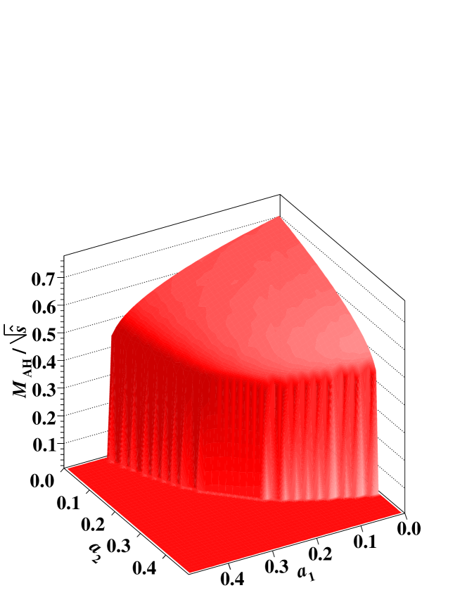
Figure 3: Relation between the horizon mass $M_{\mathrm{AH}}/\sqrt{\hat{s}}$ and the charge parameters $a_{1}$ and $a_{2}$ for $D=4$.

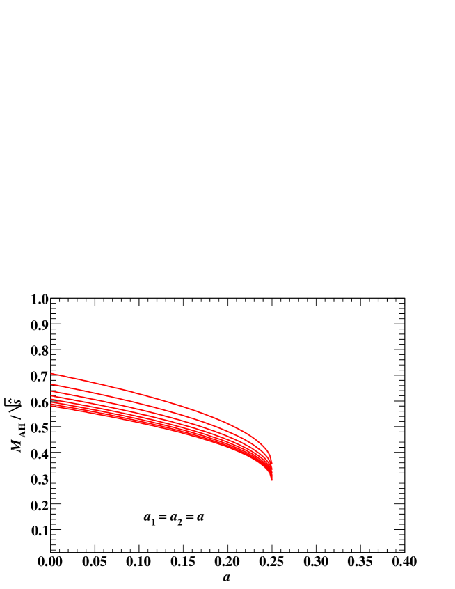
Figure 4: Relation between the horizon mass $M_{\mathrm{AH}}/\sqrt{\hat{s}}$ and the charge parameters $a_{1}=a_{2}=a$ (particles of equal charge) for $D=4,\ldots,11$.

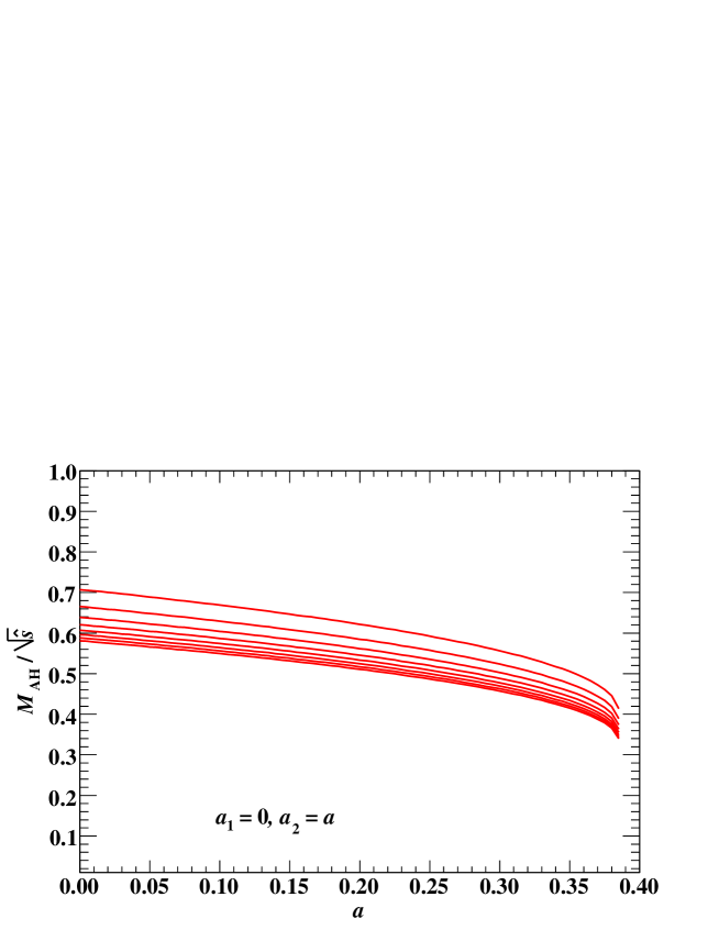
Figure 5: Relation between the horizon mass $M_{\mathrm{AH}}/\sqrt{\hat{s}}$ and the charge parameters $a_{1}=a$ and $a_{2}=0$ (one neutral particle) for $D=4,\ldots,11$.

6 Effect of charged partons on the cross section

The classical black hole cross section at the parton level is

$$\hat{\sigma}_{ab\to\mathrm{BH}}=\pi r_{\mathrm{h}}^{2}\,,$$ (35)

where $r_{\mathrm{h}}$ depends on the mass of the black hole $M_{\mathrm{BH}}$, the spacetime parameters $D$ and $M_{D}$, and $a$ and $b$ are the parton types.

Only a fraction of the total centre of mass energy $\sqrt{s}$ in a proton-proton collision is available in the parton scattering process. We define

$$sx_{a}x_{b}\equiv s\tau\equiv\hat{s}\,,$$ (36)

where $x_{a}$ and $x_{b}$ are the fractional energies of the two partons relative to the proton energies. The total cross section can be obtained by convoluting the parton-level cross section with the parton distribution functions (PDFs), integrating over the phase space, and summing over the parton types. Assuming all the available parton energy $\sqrt{\hat{s}}$ goes into forming the black hole, the full particle-level cross section is

$$\sigma_{pp\to\mathrm{BH+X}}(M_{\mathrm{BH}})=\sum_{a,b}\int_{M_{\mathrm{BH}}^{2}/s}^{1}dx_{a}\int_{M_{\mathrm{BH}}^{2}/(x_{a}s)}^{1}dx_{b}f_{a}(x_{a})f_{b}(x_{b})\hat{\sigma}_{ab\to\mathrm{BH}}(\hat{s}=M_{\mathrm{BH}})\,,$$ (37)

where $f_{a}$ and $f_{b}$ are PDFs for the proton. The sum is over all possible quark and gluon pairings.

Throughout this paper we use the CTEQ6L1 (leading order with leading order $\alpha_{s}$) parton distribution functions [28] within the LHAPDF framework [29]. The momentum scale for the PDFs is set equal to the black hole mass for convenience.

In terms of the parton luminosity (or parton flux), we write the differential form of eq. (37) as

$$\frac{d\sigma_{pp\to\mathrm{BH+X}}}{dM_{\mathrm{BH}}}=\frac{dL}{dM_{\mathrm{BH}}}\hat{\sigma}_{ab\to\mathrm{BH}}\,,$$ (38)

where

$$\frac{dL}{dM_{\mathrm{BH}}}=\frac{2M_{\mathrm{BH}}}{s}\sum_{a,b}\int_{M_{\mathrm{BH}}^{2}/s}^{1}\frac{dx}{x}f_{a}\left(\frac{\tau}{x}\right)f_{b}(x)\,.$$ (39)

The differential cross section thus factorizes. It can be written as the product of the parton cross section times a luminosity function. The parton cross section $\hat{\sigma}_{ab\to\mathrm{BH}}$ is independent of the parton types and depends only on the black hole mass, Planck scale, and number of dimensions. The parton luminosity function contains all the information about the partons. Besides a dependence on the black hole mass, it is independent of the characteristics of the higher-dimensional space, i.e. the Planck scale and number of dimensions. The dependence of the black hole mass occurs only in the proportionality and the limit of integration.

The transition from the parton-level to the hadron-level cross section is based on a factorization formula. The validity of this formula for the energy region above the Planck scale is unclear. Even if factorization is valid, the extrapolation of the parton distribution functions into this transplanckian region based on Standard Model evolution from present energies is questionable, since the evolution equations neglect gravity.

For a fixed proton-proton centre of mass energy, the parton luminosity function can be pre-calculated to obtain a function depending only on a single mass parameter. Figure 6 shows the parton luminosity function versus black hole mass for $\sqrt{s}=14$ TeV for different partons in the sum of eq. (39). The solid line is for all partons, include sea quarks and gluons. The dashed line shows the luminosity with the sea quarks removed. The doted line shows the luminosity with the sea quarks and gluons removed, and the dash-dotted line is for only gluons. Figure 6 indicates that to a good approximation, we can ignore the contribution from the sea quarks at high black hole masses. The gluon-only contribution is the lower bound on the luminosity function when the charged quarks do not contribute to the cross section.

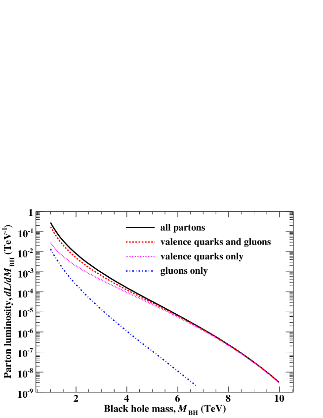
Figure 6: Different contributions to the parton luminosity function versus black hole mass.

Throughout the remainder of this analysis, we ignore the contribution to the cross section from the sea quarks. We work with parton luminosity, which is independent of $D$ and $M_{D}$. Only the condition on which quarks to include in the sum of eq. (39) depends on $D$ and $M_{D}$. Thus the upper and lower bounds on the parton luminosity do not change for different parameters. We take the running of the coupling constant into account; $\alpha$ ranges from about 1/126 to 1/122 over a black hole mass range of 1 TeV to 10 TeV. We choose $\alpha$ equal to 1/124 in the following calculations. Because of the large momentum transfer in black hole production, we use current quark masses. Quark masses of $m_{\mathrm{d}}=8$ MeV and $m_{\mathrm{u}}=4$ MeV are chosen for the valence quarks in the proton. To study eq. (39), we must first boost the partons to the equal-energy frame to calculate eq. (32), and then determine if the condition in fig. 2 is satisfied. If it is, the parton pair is included in the sum in eq. (39).

Figure 7 shows the distribution of values of the charges $a_{1}$ and $a_{2}$ for 11 dimensions, a Planck scale of 1.75 TeV, and a brane thickness of 1. Distributions for same charges, different charges, and one neutral parton combinations are clearly visible. The distributions fall off with increasing values of $a$. The maximum values of $a_{1}$ and $a_{2}$ depend on the higher-dimensional spacetime parameters $D$, $M_{D}$, and $C_{\mathrm{brane}}$. The bin representing gluon-gluon collisions $(a_{1}=a_{2}=0)$ is surrounded by a region (not visible) of no events. This vacated region increases with increasing Planck scale.

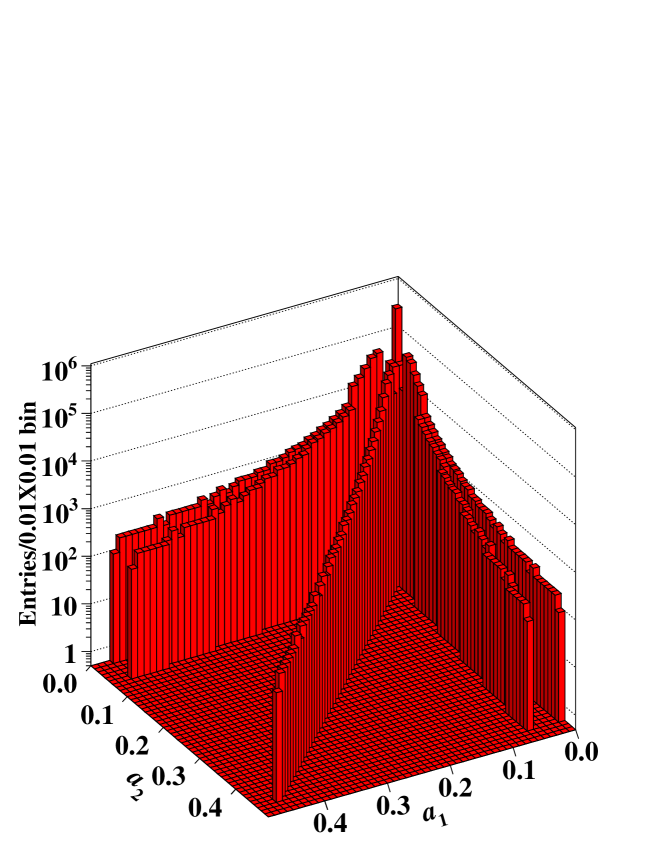
Figure 7: Histrogram of values of the particle charges $a_{1}$ and $a_{2}$ in proton-proton collisions with $D=11$, $M_{D}=1.75$ TeV, and $C_{\mathrm{brane}}=1$.

Figure 8 shows the parton luminosity for different brane thicknesses for 11 dimensions and a Planck scale of 1 TeV. The top curve is the case when all the partons contribute to the cross section, while the lower curve is the case when only the neutral gluons contribute to the cross section. The contributions of the different quarks in the intermediate region depends on $M_{\mathrm{BH}}$, $D$, $M_{D}$, and $C_{\mathrm{brane}}$. The thresholds for different quarks to contribute occur as a function of $M_{\mathrm{BH}}$ for fixed $D$, $M_{D}$, and $C_{\mathrm{brane}}$. The location of the thresholds may or may not occur in the mass region of our plot. From fig. 8, we see that charge can affect any black hole mass and the effect is very sensitive to the brane thickness. The decrease in parton luminosity, and thus cross section, can range from about one to four orders of magnitude over a black hole mass range of $1-10$ TeV due to charge effects. The cross section is nontrivial only over a range of brane thicknesses from 1.1 to 2.2. Plots with different number of dimensions are similar to fig. 8; they are always bounded above and below by the same values, but for different values of the brane thickness.

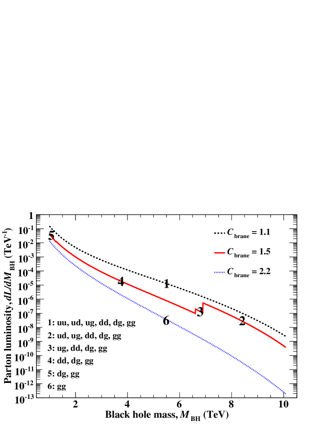
Figure 8: Parton luminosity function versus black hole mass with the charge condition applied for different brane thicknesses for $D=11$ and $M_{D}=1$ TeV. The numbers on the plot show the different parton contributions to the parton luminosity function.

For each number of dimensions, we determine the maximum brane thickness for all partons to be included in the parton luminosity and the minimum brane thickness for only gluons to be included in the parton luminosity. The results are shown in fig. 9. For a thin brane, the cross section is not affected for high dimensions. For a thick brane, the cross section is reduced for most number of dimensions. For a Planck scale of 1 TeV and a brane thickness of 1 TeV^-1, the cross section is minimal for $D\lesssim 8$, not affected for $D\gtrsim 11$, and has a range of values in the region $9\lesssim D\lesssim 10$.

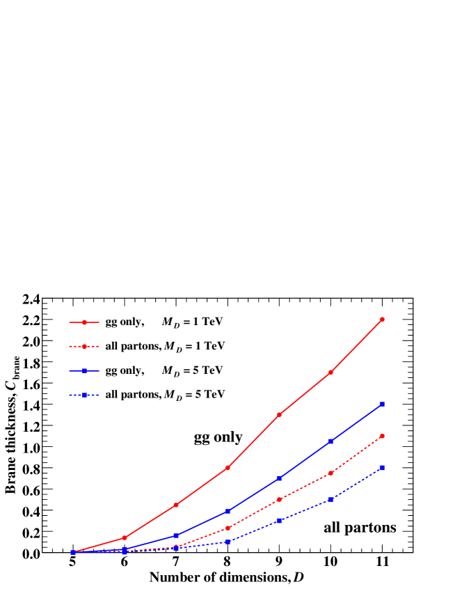
Figure 9: Brane thickness versus number of dimensions for which all quarks (dashed lines) and no quarks (solid lines) contribute to the cross section. The circles are for $M_{D}=1$ TeV and the squares are for $M_{D}=5$ TeV. No quarks contribute to the cross section in the region above the solid curves. The cross section is not affect by the charge condition below the region of the dashed curves. Some quarks contribute to the cross section in the region between the different curve types.

Using the definition of the Planck scale and electric charge, we find that the condition for a Reissner-Nordström horizon, eq. (6), becomes

$$\left|C_{q_{1}}+C_{q_{2}}\right|\leq\frac{M_{\mathrm{BH}}}{M_{D}}\frac{1}{\sqrt{\alpha}\Omega_{D-2}}\sqrt{\frac{D-3}{D-2}}\left(\frac{2\pi}{C_{\mathrm{brane}}}\right)^{\frac{D-4}{2}}\,.$$ (40)

This inequality is satisfied for $D>4$ provided the brane is not too thick. This result is contradictory to Ref. [30], where the effect of the Standard Model confinement to the three-brane seems to have been ignored. Table 1 shows upper bounds on the brane thickness for the inequality in eq. (40) to be satisfied. However, the natural thickness of the brane in models with low-scale quantum gravity can not be much larger than $C_{\mathrm{brane}}=1$, and thus it appears that the condition will always be satisfied for most natural values of the brane thickness. Our previous results indicated that a collision of two partons may not form a black hole even though the condition for a Reissner-Nordström horizon is satisfied. This is because eq. (40) is a necessary, but not sufficient, condition for black hole formation.

$D$	4	5	6	7	8	9	10	11
$C_{\mathrm{brane}}$	NA	0.8	1.8	2.5	3.1	3.5	4.1	4.4

Table 1: Maximum brane thicknesses for a Reissner-Nordström black hole to form.

The uncertainties in our analysis are large and particular values for the brane thicknesses obtained in this section should be taken with caution. However, the trends in values of brane thicknesses should be indicative of a more accurate formulation of the effects of charge on the black hole cross section.

7 Discussion

The electromagnetic interaction between the quarks could enhance or degrade black hole formation depending on the sign of the charges involved. Collisions between like-signed charged quarks will degrade black hole formation, while collisions between opposite-signed charged quarks will enhance black hole formation. It is not possible to know how effective the electromagnetic interaction is without directly computing the subsequent temporal evolution of the system.

The apparent horizon analysis was carried out in a regime where QED effects may be important and could restrict the reliability of the metric. QED effects become important when the exterior electrostatic energy of a point charge is equal to its rest mass. This condition can be written as

$$\frac{a}{r_{0}^{2(D-3)}}\ \lesssim\ \frac{\pi\Omega_{D-3}(2D-5)!!}{\Omega_{D-2}(2D-4)!!}\,.$$ (41)

The values of the right hand side range from 0.56 to 0.68 for $4\leq D\leq 11$. Since the apparent horizon occurs below $a=2/(3\sqrt{3})=0.38$, the condition given by eq. (41) is always satisfied. However, the condition for the importance of QED effects is a sufficient condition, not a necessary condition. It is possible that QED effects are important in the neighbourhood of the equality in eq. (41). We can not be sure if QED effects suppress or enhance the repulsive charge effect we have obtained.

Taking the boosted Reissner-Nordström metric as a reasonable description of ultarelativistic quarks, we have shown that charge effects will significantly decrease the rate of black hole formation at the LHC, if the brane is somewhat thick or if the dimensionality $D$ is not too large. The charge effects can be quite large because the electromagnetic energy-momentum tensor is proportional to $p_{e}^{2}\sim\gamma\alpha$ and the Lorentz factor $\gamma$ is much larger than $1/\alpha$ for ultrarelativistic quarks.

By using parton luminosity we have not had to specify the parton-level black hole cross section. As long as the cross section depends only on $M_{\mathrm{BH}}$, $D$, and $M_{D}$, our results should be applicable for any form of the parton-level cross section.

There remains a possibility that a black hole will form under collision even if there is no apparent horizon on the slice we considered, because apparent horizon formation is only a sufficient condition for black hole formation. In order to specify more detailed criteria for black hole formation, it will be necessary to study the temporal evolution of spacetime after the collision. The inclusion of the spin of the incoming particles is also required. Inclusion of QED effects and brane effects on gauge-field confinement may also be necessary.

References

- [1] N. Arkani-Hamed, S. Dimopoulos and G. Dvali, The hierarchy problem and new dimensions at a millimeter, Phys. Lett. B 429 (1998) 429 [hep-ph/9803315].
- [2] I. Antoniadis, N. Arkani-Hamed, S. Dimopoulos and G. Dvali, New dimensions at a millimeter to a fermi and superstings at a TeV, Phys. Lett. B 436 (1998) 257 [hep-ph/9804398].
- [3] N. Arkani-Hamed, S. Dimopoulos and G. Dvali, Phenomenology, astrophysics, and cosmology of theories with submillimeter dimensions and TeV scale quantum gravity, Phys. Rev. D 59 (1999) 086004 [hep-ph/9807344].
- [4] L. Randall and R. Sundrum, Large Mass Hierarchy from a Small Extra Dimension, Phys. Rev. Lett. 83 (1999) 3370 [hep-ph/9905221].
- [5] L. Randall and R. Sundrum, An Alternative to Compactification, Phys. Rev. Lett. 83 (1999) 4690 [hep-th/9906064].
- [6] S.W. Hawking, Particle Creation by Black Holes, Commun. Math. Phys. 43 (1975) 199.
- [7] T. Banks and W. Fischler, A Model for High Energy Scattering in Quantum Gravity, hep-th/9906038.
- [8] S.B. Giddings and S. Thomas, High energy colliders as black hole factories: The end of short distance physics, Phys. Rev. D 65 (2002) 056010 [hep-ph/0106219].
- [9] S. Dimopoulos and G. Landsberg, Black Holes at the Large Hadron Collider, Phys. Rev. Lett. 87 (2001) 161602 [hep-ph/0106295].
- [10] D.M. Eardley and S.B. Giddings, Classical black hole production in high-energy collisions, Phys. Rev. D 66 (2002) 044011 [gr-qc/0201034].
- [11] H. Yoshino and Y. Nambu, Black hole formation in the grazing collision of high-energy particles, Phys. Rev. D 67 (2003) 024009 [gr-qc/0209003].
- [12] E. Kohlprath and G. Veneziano, Black holes from high-energy beam-beam collisions, J. High Energy Phys. 06 (2002) 057 [gr-qc/0203093].
- [13] S.B. Giddings and V.S. Rychkov, Black holes from colliding wavepackets, Phys. Rev. D 70 (2004) 104026 [hep-th/0409131].
- [14] H. Yoshino and V.S. Rychkov, Improved analysis of black hole formation in high-energy particle collisions, Phys. Rev. D 71 (2005) 104028 [hep-th/0503171].
- [15] H. Yoshino and R.B. Mann, Black hole formation in the head-on collision of ultarelativistic charges, Phys. Rev. D 74 (2006) 044003 [gr-qc/0605131].
- [16] D.M. Gingrich, Black Hole Cross Section at the LHC, Int. J. Mod. Phys. A 21 (2006) 6653 [hep-ph/0609055].
- [17] P.C. Aichelburg and R.U. Sexl, On the Gravitational Field of a Massless Particle, Gen. Rel. Grav. 2 (1971) 303.
- [18] P.D. D’Eath and P.N. Payne, Gravitational radiation in black-hole collisions at the speed of light. I. Perturbation treatment of the axisymmetric collision, Phys. Rev. D 46 (1992) 658.
- [19] P.D. D’Eath and P.N. Payne, Gravitational radiation in black-hole collisions at the speed of light. II. Reduction to two independent variables and calculation of the second-order news function, Phys. Rev. D 46 (1992) 675.
- [20] P.D. D’Eath and P.N. Payne, Gravitational radiation in black-hole collisions at the speed of light. III. Results and conclusions, Phys. Rev. D 46 (1992) 694.
- [21] S.W. Hawking and G.F.R. Ellis, The Large Scale Structure of Space-Time, Cambridge University Press, Cambridge, England, 1973, ISBN: 0521099064.
- [22] K. Kang and H. Nastase, Planckian scattering effects and black hole production in low scenarios, Phys. Rev. D 71 (2005) 124035 [hep-th/0409099].
- [23] R. Penrose, Gravitational Collapse: the Role of General Relativity, Rivista del Nuovo Cimento 1 (1969) 252.
- [24] R. Wald, General Relativity, University of Chicago Press, Chicago, 1984, ISBN: 0226870332.
- [25] S.W. Hawking, Gravitational Radiation from Colliding Black Holes, Phys. Rev. Lett. 26 (1971) 1344.
- [26] C.O. Lousto and N. Sanchea, The curved shock wave space-time of ultrarelativistic charged particles and their scattering, Int. J. Mod. Phys. A 5 (1990) 915.
- [27] M. Ortaggio, Ultrarelativistic boost of spinning and charged black rings, J. Phys.: Conf. Ser. 33 (2006) 386.
- [28] J. Pumplin, D.R. Stump, J. Huston, H.L. Lai, P. Nadolsky and W.K. Tung, New Generation of Parton Distributions with Uncertainties from Global QCD Analysis, J. High Energy Phys. 07 (2002) 012 [hep-ph/0201195].
- [29] LHAPDF the Les Houches Accord PDF Interface, Version 5.2.2, maintained by M. Whalley; http://hepforge.cedar.ac.uk/lhapdf/
- [30] R. Casadio and B. Harms, Can black holes and naked singularities be detected in accelerators?, Int. J. Mod. Phys. A 17 (2002) 4635 [hep-th/0110255].