On the Particle Interpretation of the PVLAS Data:
Neutral versus Charged Particles

Abstract

Recently the PVLAS collaboration reported the observation of a rotation of linearly polarized laser light induced by a transverse magnetic field - a signal being unexpected within standard QED. Two mechanisms have been proposed to explain this result: production of a single (pseudo-)scalar particle coupled to two photons or pair production of light millicharged particles. In this work, we study how the different scenarios can be distinguished. We summarize the expected signals for vacuum magnetic dichroism (rotation) and birefringence (ellipticity) for the different types of particles - including new results for the case of millicharged scalars. The sign of the rotation and ellipticity signals as well as their dependencies on experimental parameters, such as the strength of the magnetic field and the wavelength of the laser, can be used to obtain information about the quantum numbers of the particle candidates and to discriminate between the different scenarios. We perform a statistical analysis of all available data resulting in strongly restricted regions in the parameter space of all scenarios. These regions suggest clear target regions for upcoming experimental tests. As an illustration, we use preliminary PVLAS data to demonstrate that near future data may already rule out some of these scenarios.

I Introduction

The absorption probability and the propagation speed of polarized light propagating in a magnetic field depends on the relative orientation between the polarization and the magnetic field. These effects are known as vacuum magnetic dichroism and birefringence, respectively, resulting from fluctuation-induced vacuum polarization.

In a pioneering experiment, the BFRT collaboration searched for these effects by shining linearly polarized laser photons through a superconducting dipole magnet. No significant signal was found, and a corresponding upper limit was placed on the rotation (dichroism) and ellipticity (birefringence) of the photon beam developed after passage through the magnetic field Semertzidis:1990qc ; Cameron:1993mr .

Recently, however, a follow-up experiment done by the PVLAS collaboration reported the observation of a rotation of the polarization plane of light after its passage through a transverse magnetic field in vacuum Zavattini:2005tm . Moreover, preliminary results presented by the PVLAS collaboration at various seminars and conferences hint also at the observation of an ellipticity (birefringence) PVLASICHEP ; Cantatore:IDM2006 .

These findings have initiated a number of theoretical and experimental activities, since the magnitude of the reported signals exceeds the standard-model expectations by far. If the observed effects are indeed true signals of vacuum magnetic dichroism and birefringence and not due to a subtle, yet unidentified systematic effect, they signal new physics beyond the standard model of particle physics.

One obvious possible explanation, and indeed the one which was also a motivation for the BFRT and PVLAS experiments, may be offered by the existence of a new light neutral spin-$0$ boson $\phi$ Maiani:1986md . In fact, this possibility has been studied in Ref. Zavattini:2005tm , with the conclusion that the rotation observed by PVLAS can be reconciled with the non-observation of a rotation and ellipticity by BFRT, if the hypothetical neutral boson has a mass in the range $m_{\phi}\sim(1-1.5)$ meV and a coupling to two photons in the range $g\sim(1.7-5.0)\times 10^{-6}$ GeV^-1.

Clearly, these values almost certainly exclude the possibility that $\phi$ is a genuine QCD axion $A$ Weinberg:1977ma ; Wilczek:1977pj . For the latter, a mass $m_{A}\sim 1$ meV implies a Peccei-Quinn symmetry Peccei:1977hh ; Peccei:1977ur breaking scale $f_{A}\sim 6\times 10^{9}$ GeV. Since, for an axion, $g\sim\alpha|E/N|/(2\pi f_{A})$ Bardeen:1977bd ; Kaplan:1985dv ; Srednicki:1985xd , one would need an extremely large ratio $|E/N|\sim 3\times 10^{7}$ of electromagnetic and color anomalies in order to arrive at an axion-photon coupling in the range suggested by PVLAS. This is far away from the predictions of any model conceived so far. Moreover, such a new, axion-like particle (ALP) must have very peculiar properties Masso:2005ym ; Jain:2005nh ; Jaeckel:2006id ; Masso:2006gc ; Mohapatra:2006pv ; Jain:2006ki in order to evade the strong constraints on its two photon coupling from stellar energy loss considerations Raffelt:1996 and from its non-observation in helioscopes such as the CERN Axion Solar Telescope (CAST) Zioutas:2004hi . A light scalar boson is furthermore constrained by upper limits on non-Newtonian forces Dupays:2006dp .

Recently, an alternative to the ALP interpretation of the PVLAS results was proposed Gies:2006ca . It is based on the observation that the photon-initiated real and virtual pair production of millicharged particles (MCPs) $\epsilon^{\pm}$ in an external magnetic field would also manifest itself as a vacuum magnetic dichroism and ellipticity. In particular, it was pointed out that the dichroism observed by PVLAS may be compatible with the non-observation of a dichroism and ellipticity by BFRT, if the millicharged particles have a small mass $m_{\epsilon}\sim 0.1$ eV and a tiny fractional electric charge $\epsilon\equiv Q_{\epsilon}/e\sim 10^{-6}$. As has been shown recently Masso:2006gc , such particles may be consistent with astrophysical and cosmological bounds (for a review, see Ref. Davidson:2000hf ), if their tiny charge arises from gauge kinetic mixing of the standard model hypercharge U(1) with additional U(1) gauge factors from physics beyond the standard model Holdom:1985ag . This appears to occur quite naturally in string theory Abel:2006qt .

It is very comforting that a number of laboratory-based low-energy tests of the ALP and MCP interpretation of the PVLAS anomaly are currently set up and expected to yield decisive results within the upcoming year. For instance, the Q&A experiment has very recently released first rotation data Chen:2006cd . Whereas the Q&A experimental setup is qualitatively similar to PVLAS, the experiment operates in a slightly different parameter region; here, no anomalous signal has been detected so far.

The interpretation of the PVLAS signal involving an ALP that interacts weakly with matter will crucially be tested by photon regeneration (sometimes called “light shining through walls”) experiments Sikivie:1983ip ; Anselm:1986gz ; Gasperini:1987da ; VanBibber:1987rq ; Ruoso:1992nx ; Ringwald:2003ns ; Gastaldi:2006fh presently under construction or serious consideration Pugnat:2005nk ; Rabadan:2005dm ; Cantatore:Patras ; Kotz:2006bw ; Baker:Patras ; Rizzo:Patras ; ALPS . In these experiments (cf. Fig. 1), a photon beam is shone across a magnetic field, where a fraction of them turns into ALPs. The ALP beam can then propagate freely through a wall or another obstruction without being absorbed, and finally another magnetic field located on the other side of the wall can transform some of these ALPs into photons — seemingly regenerating these photons out of nothing. Another probe could be provided by direct astrophysical observations of light rays traversing a pulsar magnetosphere in binary pulsar systems Dupays:2005xs .

Figure 1: Schematic view of a “light shining through a wall” experiment. (Pseudo-)scalar production through photon conversion in a magnetic field (left), subsequent travel through a wall, and final detection through photon regeneration (right).

Clearly, photon regeneration will be negligible for MCPs. Their existence, however, can be tested by improving the sensitivity of instruments for the detection of vacuum magnetic birefringence and dichroism Cameron:1993mr ; Zavattini:2005tm ; Chen:2006cd ; Rizzo:Patras ; Pugnat:2005nk ; Heinzl:2006xc . Another sensitive tool is Schwinger pair production in strong electric fields, as they are available, for example, in accelerator cavities Gies:2006hv . A classical probe for MCPs is the search for invisible orthopositronium decays Dobroliubov:1989mr ; Mitsui:1993ha , for which new experiments are currently running Badertscher:2006fm or being developed Rubbia:2004ix ; Vetter:2004fs .

From a theoretical perspective, the two scenarios are substantially different: the ALP scenario is parameterized by an effective non-renormalizable dimension-5 operator, the stabilization of which almost inevitably requires an underlying theory at a comparatively low scale, say in between the electroweak and the GUT scale. By contrast, the MCP scenario in its simplest version is reminiscent to QED; it is perturbatively renormalizable and can remain a stable microscopic theory over a wide range of scales.

The present paper is devoted to an investigation of the characteristic properties of the different scenarios in the light of all available data collected so far. A careful study of the optical properties of the magnetized vacuum can indeed reveal important information about masses, couplings and other quantum numbers of the potentially involved hypothetical particles. This is quantitatively demonstrated by global fits to all published data. For further illustrative purposes, we also present global fits which include the preliminary data made available by the PVLAS collaboration at workshops and conferences. We stress that this data is only used here to qualitatively demonstrate how the optical measurements can be associated with particle-physics properties. Definite quantitative predictions have to await the outcome of a currently performed detailed data analysis of the PVLAS collaboration. Still, the resulting fit regions can be viewed as a preliminary estimate of “target regions” for the various laboratory tests mentioned above. Moreover, the statistical analysis is also meant to help the theorists in deciding whether they should care at all about the PVLAS anomaly, and, if yes, whether there is a pre-selection of phenomenological models or model building blocks that deserve to be studied in more detail.

The paper is organized as follows. In the next section II we summarize the signals for vacuum magnetic dichroism and birefringence in presence of axion-like and millicharged particles. We use these results in Sec. III to show how the different scenarios can be distinguished from each other and how information about the quantum numbers of the potential particle candidates can be collected. In Sec. IV we then perform a statistical analysis including all current data. We also use preliminary PVLAS data to show the prospects for the near future. We summarize our conclusions in Sec. V.

II Vacuum Magnetic Dichroism, Birefringence, and Photon Regeneration

We start here with some general kinematic considerations relevant to dichroism and birefringence, which are equally valid for the case of ALP and the case of MCP production.

Let $\vec{k}$ be the momentum of the incoming photon, with $|\vec{k}|=\omega$, and let $\vec{B}$ be a static homogeneous magnetic field, which is perpendicular to $\vec{k}$, as it is the case in all of the afore-mentioned polarization experiments.

The photon-initiated production of an ALP with mass $m_{\phi}$ or an MCP with mass $m_{\epsilon}$, leads, for $\omega>m_{\phi}$ or $\omega>2m_{\epsilon}$, respectively, to a non-trivial ratio of the survival probabilities $\exp(-\pi_{\parallel,\perp}(\ell))$ of a photon after it has traveled a distance $\ell$, for photons polarized parallel $\parallel$ or perpendicular $\perp$ to $\vec{B}$. This non-trivial ratio manifests itself directly in a dichroism: for a linearly polarized photon beam, the angle $\theta$ between the initial polarization vector and the magnetic field will change to $\theta+\Delta\theta$ after passing a distance $\ell$ through the magnetic field, with

$$\cot(\theta+\Delta\theta)=\frac{E_{\parallel}}{E_{\perp}}=\frac{E^{0}_{\parallel}}{E^{0}_{\perp}}\exp\left(-\frac{1}{2}(\pi_{\parallel}(\ell)-\pi_{\perp}(\ell))\right).$$ (1)

Here, $E_{\parallel,\perp}$ are the electric field components of the laser parallel and perpendicular to the external magnetic field, and the superscript “0” denotes initial values. For small rotation angle $\Delta\theta$, we have

$$\Delta\theta\simeq\frac{1}{4}(\pi_{\parallel}-\pi_{\perp})\,\sin(2\theta).$$ (2)

We will present the results for the probability exponents $\pi_{\parallel}-\pi_{\perp}$ for ALPs and MCPs in the following subsections.

Let us now turn to birefringence. The propagation speed of the laser photons is slightly changed in the magnetic field owing to the coupling to virtual ALPs or MCPs. Accordingly, the time $\tau_{\parallel,\perp}(\ell)$ it takes for a photon to traverse a distance $\ell$ differs for the two polarization modes, causing a phase difference between the two modes,

$$\Delta\phi=\omega(\tau_{\parallel}(\ell)-\tau_{\perp}(\ell)).$$ (3)

This induces an ellipticity $\psi$ of the outgoing beam,

$$\psi=\frac{\omega}{2}(\tau_{\parallel}(\ell)-\tau_{\perp}(\ell))\sin(2\theta),\quad\quad\rm{for}\,\,\psi\ll 1.$$ (4)

Again, we will present the results for $\tau_{\parallel}-\tau_{\perp}$ for ALPs and MCPs in the following subsections.

II.1 Production of Neutral Spin-0 Bosons

A neutral spin-0 particle can interact with two photons via

$${\mathcal{L}}^{(+)}_{\rm{int}}=-\frac{1}{4}g\phi^{(+)}F_{\mu\nu}F^{\mu\nu}=\frac{1}{2}g\phi^{(+)}(\vec{E}^{2}-\vec{B}^{2}),$$ (5)

if it is a scalar, or

$${\mathcal{L}}^{(-)}_{\rm{int}}=-\frac{1}{4}g\phi^{(-)}F_{\mu\nu}\widetilde{F}^{\mu\nu}=g\phi^{(-)}(\vec{E}\cdot\vec{B}),$$ (6)

if it is a pseudoscalar. In a homogeneous magnetic background $\vec{B}$, the leading order contribution to the conversion (left half of Fig. 1) of (pseudo-)scalars into photons comes from the terms $\sim\vec{B}^{2}$ and $\sim\vec{E}\cdot\vec{B}$, respectively. The polarization of a photon is now given by the direction of the electric field of the photon, $\vec{E}_{\gamma}$, whereas its magnetic field, $\vec{B}_{\gamma}$ is perpedicular to the polarization. Therefore, only those fields polarized perpendicular (parallel) to the background magnetic field will have nonvanishing $\vec{B}_{\gamma}\cdot\vec{B}\neq 0$ ($\vec{E}_{\gamma}\cdot\vec{B}\neq 0$) and interact with the (pseudo-)scalar particles. Accordingly, for scalars we have,

$$\pi^{(+)}_{\perp}\neq 0,\quad\pi^{(+)}_{\parallel}=0,\quad\tau^{(+)}_{\perp}\neq 0,\quad\tau^{(+)}_{\parallel}=0$$ (7)

whereas for pseudoscalars we find

$$\pi^{(-)}_{\perp}=0,\quad\pi^{(-)}_{\parallel}\neq 0,\quad\tau^{(-)}_{\perp}=0,\quad\tau^{(-)}_{\parallel}\neq 0.$$ (8)

Apart from this, the interaction is identical in lowest order,

$$\pi^{(+)}_{\perp}=\pi^{(-)}_{\parallel}\,\,{\rm{and}}\,\,\tau^{(+)}_{\perp}=\tau^{(-)}_{\parallel}.$$ (9)

Using Eqs. (1)-(4) we deduce

$${{\Delta\theta}}^{(+)}=-{{\Delta\theta}}^{(-)},\,\,{\rm{and}}\,\,\psi^{(+)}=-\psi^{(-)}.$$ (10)

We can now summarize the predictions on the rotation ${{\Delta\theta}}$ and the ellipticity $\psi$ in (pseudo-)scalar ALP models with coupling $g$ and mass $m_{\phi}$ Maiani:1986md ; Raffelt:1987im . We assume a setup as in the BFRT experiment with a dipole magnet of length $L$ and homogeneous magnetic field $B$. The polarization of the laser beam with photon energy $\omega$ has an angle $\theta$ relative to the magnetic field. The effective number of passes of photons in the dipole is $N_{\text{pass}}$. Due to coherence, the rotation ${{\Delta\theta}}$ and ellipticity $\psi$ depend non-linearly on the length of the apparatus $L$ and linearly on the number of passes $N_{\rm{pass}}$, instead of simply being proportional to $\ell=N_{\rm pass}L$; whereas the photon component is reflected at the cavity mirrors, the ALP component is not and leaves the cavity after each pass:

$$-{{\Delta\theta}}^{(+)}={{\Delta\theta}}^{(-)}=N_{\text{pass}}\left(\frac{gB\omega}{m_{\phi}^{2}}\right)^{2}\sin^{2}\left(\frac{Lm_{\phi}^{2}}{4\omega}\right)\sin 2\theta,$$ (11)

$$-\psi^{(+)}\!\! = \!\!\psi^{(-)}$$

$$= \!\!\frac{N_{\text{pass}}}{2}\left(\frac{gB\omega}{m_{\phi}^{2}}\right)^{2}\left(\frac{Lm_{\phi}^{2}}{2\omega}-\sin\left(\frac{Lm_{\phi}^{2}}{2\omega}\right)\right)\sin 2\theta.$$

For completeness, we present here also the flux of regenerated photons in a “light-shining through a wall” experiment (cf. Fig. 1). In the case of a pseudoscalar, it reads

$$\dot{N}_{\gamma\ {\rm reg}}^{(-)}=\dot{N_{0}}\left\lfloor\frac{N_{\text{pass}}+1}{2}\right\rfloor\frac{1}{16}\left(gBL\cos\theta\right)^{4}\left(\frac{\sin(\frac{Lm_{\phi}^{2}}{4\omega})}{\frac{Lm_{\phi}^{2}}{4\omega}}\right)^{4},$$ (13)

where $\dot{N}_{0}$ is the original photon flux. For a scalar, the $\cos\theta$ is replaced by a $\sin\theta$. Equation (13) is for the special situation in which a dipole of length $L$ and field $\vec{B}$ is used for generation as well as for regeneration of the ALPs as it is the case for the BFRT experiment. Note that only passes towards the wall count.

II.2 Optical Vacuum Properties from Charged-Particle Fluctuations

Let us now consider the interactions between the laser beam and the magnetic field mediated by fluctuations of particles with charge $\epsilon e$ and mass $m_{\epsilon}$. For laser frequencies above threshold, $\omega>2m_{\epsilon}$, pair production becomes possible in the magnetic field, resulting in a depletion of the incoming photon amplitude. The corresponding photon attenuation coefficients $\kappa_{\|,\bot}$ for the two polarization modes are related to the probability exponents $\pi_{\|,\bot}$ by

$$\pi_{\|,\bot}=\kappa_{\|,\bot}\,\ell,$$ (14)

depending linearly on the optical path length $\ell$. Also the time $\tau_{\|,\bot}$ it takes for the photon to traverse the interaction region with the magnetic field exhibits the same dependence,

$$\tau_{\|,\bot}=n_{\|,\bot}\,\ell,$$ (15)

where $n_{\|,\bot}$ denotes the refractive indices of the magnetized vacuum.

II.2.1 Dirac Fermions

We begin with vacuum polarization and pair production of charged Dirac fermions Gies:2006ca , arising from an interaction Lagrangian

$${\mathcal{L}}_{\rm int}^{\rm Dsp}=\epsilon\,e\,\overline{\psi}_{\epsilon}\gamma_{\mu}\psi_{\epsilon}A^{\mu},$$ (16)

with $\psi_{\epsilon}$ being a Dirac spinor (“Dsp”).

Explicit expressions for the photon absorption coefficients $\kappa_{\parallel,\perp}$ can be inferred from the polarization tensor which is obtained by integrating over the fluctuations of the $\psi_{\epsilon}$ field. This process $\gamma\to\epsilon^{+}\epsilon^{-}$ has been studied frequently in the literature for the case of a homogeneous magnetic field Toll:1952 ; Klepikov:1954 ; Erber:1966vv ; Baier:1967 ; Klein:1968 ; Adler:1971wn ; Tsai:1974fa ; Daugherty:1984tr ; Dittrich:2000zu :

$$\pi_{\|,\bot}^{\rm Dsp} \equiv\kappa_{\parallel,\perp}^{\rm Dsp}\ell=\frac{1}{2}\epsilon^{3}e\alpha\frac{B\ell}{m_{\epsilon}}\,T_{\parallel,\perp}^{\rm Dsp}(\chi)$$ (17)

$$=1.09\times 10^{6}\ \epsilon^{3}\left(\frac{\rm eV}{m_{\epsilon}}\right)\left(\frac{B}{\rm T}\right)\left(\frac{\ell}{\rm m}\right)\,T_{\parallel,\perp}^{\rm Dsp}(\chi),$$

where $\alpha=e^{2}/4\pi$ is the fine-structure constant. Here, $T_{\parallel,\perp}^{\rm Dsp}(\chi)$ has the form of a parametric integral Tsai:1974fa ,

$$T_{\parallel,\perp}^{\rm Dsp}=\frac{4\sqrt{3}}{\pi\chi}\int\limits_{0}^{1}{\rm d}v\ K_{2/3}\left(\frac{4}{\chi}\frac{1}{1-v^{2}}\right)\\ \times\frac{\left[\left(1-\frac{1}{3}v^{2}\right)_{\parallel},\left(\frac{1}{2}+\frac{1}{6}v^{2}\right)_{\perp}\right]}{(1-v^{2})}$$ (18)

$\displaystyle=\begin{cases}\sqrt{\frac{3}{2}}\ {\rm e}^{-4/\chi}\ \left[(\frac{1}{2})_{\parallel},(\frac{1}{4})_{\perp}\right]&\text{for}\,\,\chi\ll 1\,\,\text{,}\\ \frac{2\pi}{\Gamma\left(\frac{1}{6}\right)\Gamma\left(\frac{13}{6}\right)}\chi^{-1/3}\left[(1)_{\parallel},(\frac{2}{3})_{\perp}\right]&\text{for}\,\,\chi\gg 1\,\,\text{,}\end{cases}$

the dimensionless parameter $\chi$ being defined as

$$\chi\equiv\frac{3}{2}\frac{\omega}{m_{\epsilon}}\frac{\epsilon eB}{m_{\epsilon}^{2}}=88.6\ \epsilon\ \frac{\omega}{m_{\epsilon}}\ \left(\frac{\rm eV}{m_{\epsilon}}\right)^{2}\left(\frac{B}{\rm T}\right)\,.$$ (19)

The above expression has been derived in leading order in an expansion for high frequency Toll:1952 ; Klepikov:1954 ; Erber:1966vv ; Baier:1967 ; Klein:1968 ; Heinzl:2006pn ,

$$\frac{\omega}{2m_{\epsilon}}\gg 1,$$ (20)

and of high number of allowed Landau levels of the millicharged particles Daugherty:1984tr ,

$$\Delta N_{\rm{p}}\!\! = \!\!\frac{\Delta N_{\rm{Landau}}}{2}=\frac{1}{12}\left(\frac{\omega^{2}}{\epsilon\,eB}\right)^{2}\left(\frac{\Delta\omega}{\omega}+\frac{\Delta B}{2B}\right)\gg 1$$

$$\Leftrightarrow\epsilon\!\! \ll \!\!4.9\times 10^{-3}\left(\frac{\omega}{\rm{eV}}\right)^{2}\left(\frac{\rm{T}}{B}\right)\left(\frac{\Delta\omega}{\omega}+\frac{\Delta B}{2B}\right)^{\frac{1}{2}}.$$ (21)

In the above-mentioned laser polarization experiments, the variation $\Delta\omega/\omega$ is typically small compared to $\Delta B/B\gtrsim 10^{-4}$.

Virtual production can occur even below threshold, $\omega<2m_{\epsilon}$. Therefore, we consider both high and low frequencies. As long as Eq. (21) is satisfied, one has Tsai:1975iz

$$n_{\parallel,\perp}^{\rm Dsp}=1-\frac{\epsilon^{2}\alpha}{4\pi}\left(\frac{\epsilon\,eB}{m^{2}_{\epsilon}}\right)^{2}I_{\parallel,\perp}^{\rm Dsp}(\chi),$$ (22)

with

$$I_{\parallel,\perp}^{\rm Dsp}(\chi)\!\!=\!\!2^{\frac{1}{3}}\left(\frac{3}{\chi}\right)^{\frac{4}{3}}\int^{1}_{0}{\rm d}v\,\frac{\left[\left(1-\frac{v^{2}}{3}\right)_{\parallel},\left(\frac{1}{2}+\frac{v^{2}}{6}\right)_{\perp}\right]}{(1-v^{2})^{\frac{1}{3}}}\\ \times\tilde{e}^{\prime}_{0}\left[\scriptstyle-\left(\frac{6}{\chi}\frac{1}{1-v^{2}}\right)^{\frac{2}{3}}\right]$$ (23)

$\displaystyle=\begin{cases}-\frac{1}{45}\left[(14)_{\parallel},(8)_{\perp}\right]&\text{for}\,\,\chi\ll 1\text{,}\\ \frac{9}{7}\frac{\pi^{\frac{1}{2}}2^{\frac{1}{3}}\left(\Gamma(\left(\frac{2}{3}\right)\right)^{2}}{\Gamma\left(\frac{1}{6}\right)}\chi^{-4/3}\left[(3)_{\parallel},(2)_{\perp}\right]&\text{for}\,\,\chi\gg 1\text{.}\end{cases}$

Here, $\tilde{e}_{0}$ is the generalized Airy function,

$$\tilde{e}_{0}(t)=\int^{\infty}_{0}{\rm d}x\,\sin\left(tx-\frac{x^{3}}{3}\right),$$ (24)

and $\tilde{e}^{\prime}_{0}(t)={\rm{d}}\tilde{e}_{0}(t)/{\rm{d}}t$.

II.2.2 Spin-0 Bosons

The optical properties of a magnetized vacuum can also be influenced by fluctuations of charged spin-0 bosons. The corresponding interaction Lagrangian is that of scalar QED (index “sc”),

$${\mathcal{L}}^{\rm sc}=-|D_{\mu}(\epsilon eA)\varphi_{\epsilon}|^{2}-m_{\epsilon}^{2}|\varphi_{\epsilon}|^{2},\quad D_{\mu}=\partial_{\mu}-\text{i}\epsilon eA_{\mu},$$ (25)

with $\varphi_{\epsilon}$ being a complex scalar field. The induced optical properties have not been explicitly computed before in the literature, but can be inferred straightforwardly from the polarization tensor found in Schubert:2000yt . As derived in more detail in appendices A and B, the corresponding results for dichroism and birefringence are similar to the familiar Dirac fermion case,

$$\pi_{\|,\bot}^{\rm sc}\equiv\kappa_{\parallel,\perp}^{\rm sc}\ell=\frac{1}{2}\epsilon^{3}e\alpha\frac{B\ell}{m_{\epsilon}}\,T_{\parallel,\perp}^{\rm sc}(\chi),$$ (26)

where

$$T_{\parallel,\perp}^{\text{sc}}=\frac{2\sqrt{3}}{\pi\chi}\int\limits_{0}^{1}{\rm d}v\ K_{2/3}\left(\frac{4}{\chi}\frac{1}{1-v^{2}}\right)\\ \times\frac{\left[\left(\frac{1}{3}v^{2}\right)_{\parallel},\left(\frac{1}{2}-\frac{1}{6}v^{2}\right)_{\perp}\right]}{(1-v^{2})}$$ (27)

$\displaystyle=\begin{cases}\frac{1}{2}\sqrt{\frac{3}{2}}\ {\rm e}^{-4/\chi}\ \left[(0)_{\parallel},(\frac{1}{4})_{\perp}\right]&\text{for}\,\,\chi\ll 1\,\,\text{,}\\ \frac{\pi}{\Gamma\left(\frac{1}{6}\right)\Gamma\left(\frac{13}{6}\right)}\chi^{-1/3}\left[(\frac{1}{6})_{\parallel},(\frac{1}{2})_{\perp}\right]&\text{for}\,\,\chi\gg 1\,\,\text{.}\end{cases}$

The zero coefficient in Eq. (27) holds, of course, only to leading order in this calculation. We observe that the $\bot$ mode dominates absorption in the scalar case in contrast to the spinor case. Hence, the induced rotation of the laser probe goes into opposite directions in the two cases, bosons and fermions.

The refractive indices induced by scalar fluctuations read

$$n_{\parallel,\perp}^{\rm sc}=1-\frac{\epsilon^{2}\alpha}{4\pi}\left(\frac{\epsilon\,eB}{m^{2}_{\epsilon}}\right)^{2}I_{\parallel,\perp}^{\rm sc}(\chi),$$ (28)

with

$$I_{\parallel,\perp}^{\text{sc}}(\chi)\!\!=\frac{2^{\frac{1}{3}}}{2}\left(\frac{3}{\chi}\right)^{\frac{4}{3}}\int^{1}_{0}{\rm d}v\,\frac{\left[\left(\frac{v^{2}}{3}\right)_{\parallel},\left(\frac{1}{2}-\frac{v^{2}}{6}\right)_{\perp}\right]}{(1-v^{2})^{\frac{1}{3}}}\\[6.45831pt] {\times\tilde{e}^{\prime}_{0}\left[\scriptstyle-\left(\frac{6}{\chi}\frac{1}{1-v^{2}}\right)^{\frac{2}{3}}\right]}$$ (29)

$\displaystyle=\begin{cases}-\frac{1}{90}\left[(1)_{\parallel},(7)_{\perp}\right]&\text{for}\,\,\chi\ll 1\,\,\text{,}\\ \frac{9}{14}\frac{\pi^{\frac{1}{2}}2^{\frac{1}{3}}\left(\Gamma\left(\frac{2}{3}\right)\right)^{2}}{\Gamma\left(\frac{1}{6}\right)}\chi^{-4/3}\left[(\frac{1}{2})_{\parallel},(\frac{3}{2})_{\perp}\right]&\text{for}\,\,\chi\gg 1\,\,\text{.}\end{cases}$

Again, the polarization dependence of the refractive indices renders the magnetized vacuum birefringent. We observe that the induced ellipticities for the scalar and the spinor case go into opposite directions. In particular, for small $\chi$, the $\bot$ mode is slower for the scalar case, supporting an ellipticity signal which has the same sign as that of Nitrogen. For the spinor case, it is the other way round. As a nontrivial cross-check of our results for the scalar case, note that the refractive indices for $\chi\ll 1$ precisely agree with the (inverse) velocities computed in Eqs. (50) and (51) from the Heisenberg-Euler effective action of scalar QED.

We conclude that a careful determination of the signs of ellipticity and rotation in the case of a positive signal can distinguish between spinor and scalar fluctuating particles.

Finally, let us briefly comment on the case of having both fermions and bosons. If there is an identical number of bosonic and fermionic degrees of freedom with exactly the same masses and millicharges, i.e. if the millicharged particles appear in a supersymmetric fashion in complete supersymmetric chiral multiplets, one can check that the signals cancel. An exactly supersymmetric set of millicharged particles would cause neither an ellipticity signal nor a rotation of the polarization and one would have to rely on other detection principles as, for example, Schwinger pair production in accelerator cavities Gies:2006hv . However, in nature supersymmetry is broken resulting in different masses for bosons and fermions. Now, the signal typically decreases rather rapidly for large masses (more precisely when $\chi\sim 1/m^{3}_{\epsilon}$ becomes smaller than one) and the lighter particle species will give a much bigger contribution. Accordingly, for a sufficiently large mass splitting the signal would look more or less as if we had only the lighter particle species, be it a fermion or a boson.

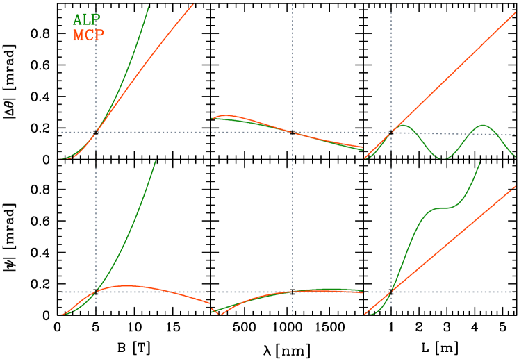
Figure 2: Dependence of the rotation and ellipticity signals on the strength of the magnetic field $B$, the wavelength $\lambda$ of the laser, and the length $L$ of the magnetic region inside the cavity. For ALPs (dark green) and MCPs (light red). The crossing of the blue dotted lines corresponds to the PVLAS published rotation and preliminary ellipticity signal for $B=5$ T, $\lambda=1064$ nm, and $L=1$ m.

III Distinguishing between different Scenarios

In principle, one can set up a series of different experiments distinguishing between the different scenarios, ALPs or MCPs. For example, a positive signal in a light-shining-through-wall experiment Sikivie:1983ip ; Anselm:1986gz ; Gasperini:1987da ; VanBibber:1987rq ; Ruoso:1992nx ; Ringwald:2003ns ; Gastaldi:2006fh ; Pugnat:2005nk ; Rabadan:2005dm ; Cantatore:Patras ; Kotz:2006bw ; Baker:Patras ; Rizzo:Patras ; ALPS would be a clear signal for the ALP interpretation, whereas detection of a dark current that is able to pass through walls would be a clear signal for the MCP hypothesis Gies:2006hv . But even with a PVLAS-type experiment that measures only the rotation and ellipticity signals, one can collect strong evidence favoring one and disfavoring other scenarios.

	$n_{\|}>n_{\bot}$	$n_{\|}<n_{\bot}$
$\pi_{\|}>\pi_{\bot}$	ALP 0- or MCP $\frac{1}{2}$ (small $\chi$)	MCP $\frac{1}{2}$ (large $\chi$)
$\pi_{\|}<\pi_{\bot}$	MCP $0$ (large $\chi$)	ALP 0+ or MCP $0$ (small $\chi$)

Table 1: Summary of the allowed particle-physics interpretation arising from a sign analysis of birefringence induced by different refractive indices $n_{\|,\bot}$ and dichroism induced by different probability exponents $\pi_{\|,\bot}$.

Performing one measurement of the absolute values of rotation and ellipticity, one can typically find values for the masses and couplings in all scenarios, such that the predicted rotation and ellipticity is in agreement with the experiment.

One clear distinction can already be made by measuring the sign of the ellipticity and rotation signals. In the ALP scenario, a measurement of the sign of either the rotation or the ellipticity is sufficient to decide between a scalar or pseudoscalar. Measuring the sign of both signals already is a consistency check; if the signal signs turn out to be inconsistent, the ALP scenarios for both the scalar and the pseudoscalar would be ruled out. In the MCP scenario, a measurement of the sign of rotation decides between scalars and fermions. If only the sign of the ellipticity signal is measured, both options still remain, since the sign of the ellipticity changes when one moves from large to small masses: the hierarchy of the refractive indices is inverted in the region of anomalous dispersion. But at least the sign tells us if we are in the region of large or small masses, corresponding to a small or large $\chi$ parameter, cf. Eq. (19). This sign analysis is summarized in Table 1.

More information can be obtained by varying the parameters of the experiment. In principle, we can vary all experimental parameters appearing in Eqs. (11), (II.1), (17) and (22): the strength of the magnetic field $B$, the frequency of the laser $\omega$, and the length of the magnetic field inside the cavity ${L}$.

Let us start with the magnetic field dependence. For the ALP scenario both rotation and ellipticity signals are proportional to $B^{2}$,

$$\Delta\theta^{\text{ALP}}\sim B^{2},\quad\psi^{\text{ALP}}\sim B^{2}$$ (30)

whereas for MCP’s we have

$$\Delta\theta^{\text{MCP}}\!\! \sim \!\!\bigg{\{}\begin{array}[]{ll}\exp\left(-\frac{\text{const}}{B}\right)&\quad B\,\,\text{small}\\ B^{\frac{2}{3}}&\quad B\,\,\text{large}\end{array}$$ (33)

$$\psi^{\text{MCP}}\!\! \sim \!\!\bigg{\{}\begin{array}[]{ll}B^{2}&\quad B\,\,\text{small}\\ B^{\frac{2}{3}}&\quad B\,\,\text{large}.\\ \end{array}$$ (36)

In the left panels of Fig. 2 we demonstrate the different behavior (for the ellipticity signal the $B^{\frac{2}{3}}$-dependence is not yet visible as it appears only at much stronger fields). The model parameters for ALPs and MCPs are chosen such that the absolute value of $\Delta\theta$ and $\psi$ matches the PVLAS results ($\lambda=1064$ nm, $B=5$ T, and $L=1$ m) shown as the crossing of the dotted lines together with their statistical errors. In a similar manner, the signals also depend on the wavelength of the laser light, which is shown in the center panels of Fig. 2.

Finally, there is one more crucial difference between the ALP and the MCP scenario. Production of a single particle can occur coherently. This leads to a faster growth of the signal

$$\Delta\theta^{\text{ALP}}\sim{L}^{2},\quad\psi^{\text{ALP}}\sim{L}^{2}\quad\,\,{L}\,\,\text{small}.$$ (37)

In the MCP scenario, however, the produced particles are essentially lost and we have only a linear dependence on the length of the interaction region,

$$\Delta\theta^{\text{MCP}}\sim{L},\quad\psi^{\text{MCP}}\sim{L}.$$ (38)

This is shown in the right panels of Fig. 2.

We conclude that studying the dependence of the signal on the parameters of the experiment can give crucial information to decide between the ALP and MCP scenarios, as we will also see in the following section.

BFRT experiment
Rotation ($L=8.8$ m, $\lambda=514.5$ nm, $\theta=\nicefrac{{\pi}}{{4}}$)
$N_{\text{pass}}$	$\left|{\Delta\theta}\right|\,[\text{nrad}]$	${\Delta\theta}_{\text{noise}}\,[\text{nrad}]$
$254$	$0.35$	$0.30$
$34$	$0.26$	$0.11$
Ellipticity ($L=8.8$ m, $\lambda=514.5$ nm, $\theta=\nicefrac{{\pi}}{{4}}$)
$N_{\text{pass}}$	$\left|\psi\right|\,[\text{nrad}]$	$\psi_{\text{noise}}\,[\text{nrad}]$
$578$	$40.0$	$11.0$
$34$	$1.60$	$0.44$
Regeneration ($L=4.4$ m, $\langle\lambda\rangle=500$ nm, $N_{\text{pass}}=200$)
$\theta\,[\text{rad}]$	rate $[\text{Hz}]$
$0$	$-0.012\pm 0.009$
$\nicefrac{{\pi}}{{2}}$	$0.013\pm 0.007$

Table 2: The vacuum rotation ${\Delta\theta}$, ellipticity $\psi$ and photon regeneration rate from the BFRT Cameron:1993mr experiment. For simplicity we take the noise level ${\Delta\theta}_{\text{noise}}$ and $\psi_{\text{noise}}$ quoted in Ref. Cameron:1993mr as the standard deviation $\sigma_{\Delta\theta}$ and $\sigma_{\psi}$. For the polarization data, BFRT used a magnetic field with time-varying amplitude $B=B_{0}+\Delta B\cos(\omega_{m}t+\phi_{m})$, where $B_{0}=3.25$ T and $\Delta B=0.62$ T (cf. Appendix C). For photon regeneration, they employed $B=3.7$ T.

IV Confrontation with Data

In this Section, we want to confront the prediction of the ALP and MCP scenarios for vacuum magnetic dichroism, birefringence, and photon regeneration with the corresponding data from the BFRT Cameron:1993mr and PVLAS Zavattini:2005tm ; PVLASICHEP ; Cantatore:IDM2006 collaborations, as well as from the Q&A experiment Chen:2006cd . The corresponding experimental findings are summarized in Tables 2, 3, and 4, respectively.

PVLAS experiment
Rotation ($L=1$ m, $N_{\text{pass}}=44000$, $\theta=\nicefrac{{\pi}}{{4}}$)
$\lambda\,\,[\text{nm}]$	$\left|{\Delta\theta}\right|\,[10^{-12}\,\text{rad}/\text{pass}]$
$1064$	$3.9\pm 0.2$
$532$	$6.3\pm 1.0$ (preliminary)
Ellipticity ($L=1$ m, $N_{\text{pass}}=44000$, $\theta=\nicefrac{{\pi}}{{4}}$)
$\lambda\,\,[\text{nm}]$	$\psi\,[10^{-12}\,\text{rad}/\text{pass}]$
$1064$	$-3.4\pm 0.3$ (preliminary)
$532$	$-6.0\pm 0.6$ (preliminary)

Table 3: The vacuum rotation ${\Delta\theta}$ and ellipticity $\psi$ per pass measured by PVLAS, for $B=5$ T. The rotation of polarized laser light with $\lambda=1064$ nm is published in Ref. Zavattini:2005tm . Preliminary results are taken from Refs. PVLASICHEP ; Cantatore:IDM2006 and are used here for illustrative purposes only.

Q&A experiment
Rotation ($L=1$ m, $\lambda=1064$ nm, $\theta=\nicefrac{{\pi}}{{4}}$)
$N_{\text{pass}}$	$\Delta\theta\,[\text{nrad}]$
$18700$	$-0.4\pm 5.3$

Table 4: The vacuum rotation ${\Delta\theta}$ from the Q&A experiment Chen:2006cd experiment ($B=2.3$ T).

In the following we combine these results in a simple statistical analysis. For simplicity, we assume that the likelihood function $L_{i}$ of the rotation, the ellipticity and the photon regeneration rate follows a Gaussian distribution in each measurement $i$ with mean value and standard deviation as indicated in Tables 2-4. In the case of the BFRT upper limits, we approximate the likelihood functions by $L\propto\exp((\psi-\psi_{\text{hypo}})^{2}/(2\psi_{\text{noise}}^{2}))$. Taking these inputs as statistically independent values we can estimate the combined log-likelihood function as $\ln L\approx\sum_{i}\ln L_{i}$ Yao:2006px . With these assumptions the method of maximum likelihood is equivalent to the method of least squares with $\chi^{2}=\text{const}-2\sum_{i}\ln L_{i}$. A more sophisticated statistical analysis is beyond the scope of this work and requires detailed knowledge of the data analysis.

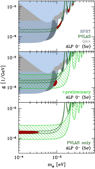
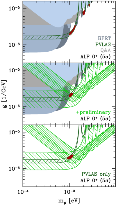
Figure 3: ALP: The $5\sigma$ confidence level of the model parameters (red). The blue shaded regions arise from the BFRT upper limits for regeneration (darkblue), rotation (blue) and ellipticity (lightblue). The gray shaded region is the Q&A upper limit for rotation. The bands show the PVLAS $5\sigma$ C.L.s for rotation (coarse-hatched) and ellipticity (fine-hatched) with $\lambda=532$ nm (left-hatched) and $\lambda=1064$ nm (right-hatched), respectively. The darkgreen band shows the published result for rotation with $\lambda=1064$ nm. The lightgreen bands result from an inclusion of preliminary data from PVLAS. The upper panels show the fit to the published data; the center panels include also the preliminary data from PVLAS, and the lower panels depict the fit using only PVLAS data. The preliminary data is only used to demonstrate the potential to distinguish between the different scenarios.

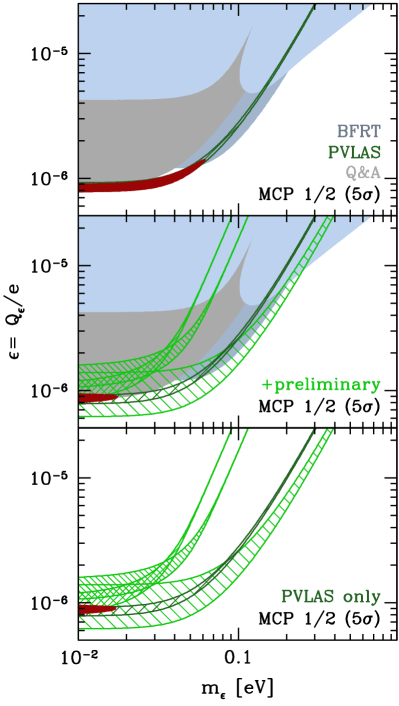
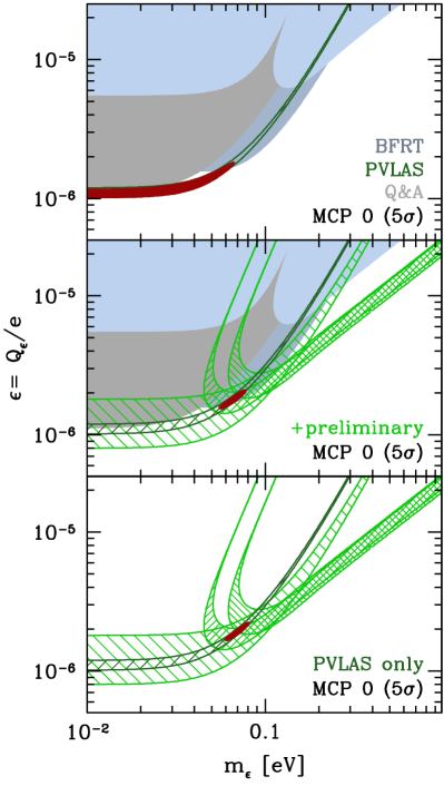
Figure 4: MCP: The $5\sigma$ confidence level of the model parameters (red). The blue shaded regions arise from the BFRT upper limits for rotation (blue) and ellipticity (lightblue). The gray shaded region is the Q&A upper limit for rotation. The bands show the PVLAS $5\sigma$ C.L.s for rotation (coarse-hatched) and ellipticity (fine-hatched) with $\lambda=532$ nm (left-hatched) and $\lambda=1064$ nm (right-hatched), respectively. The darkgreen band shows the published result for rotation with $\lambda=1064$ nm. The lightgreen bands result from an inclusion of preliminary data from PVLAS. The upper panels show the fit to the published data; the center panels include also the preliminary data from PVLAS, and the lower panels depict the fit using only PVLAS data. The preliminary data is only used to demonstrate the potential to distinguish between the different scenarios. The preliminary PVLAS value for the sign of the ellipticity singles out the large-$\chi$ (small-mass) branch of the fermionic MCP $\frac{1}{2}$ and the small-$\chi$ (large-mass) branch of the scalar MCP 0, cf. Table 1, as is visible in the center and lower panels.

IV.1 ALP hypothesis

$\chi^{2}/$d.o.f.	ALP 0-	ALP 0+	MCP $\frac{1}{2}$	MCP 0
BFRT, PVLAS, Q&A published data (d.o.f.$=6$)	1.3	0.8	7.4	7.3
+ PVLAS preliminary data (d.o.f.$=9$)	62.0	6.3	15.7	12.0
only PVLAS pub. + prelim. data (d.o.f.$=2$)	118.4	18.9	40.0	15.7

Table 5: Summary of the $\chi^{2}$/d.o.f. analysis for the different scenarios and based on different data sets. Rows and columns correspond to the rows and columns of panels in Figs. 3 and 4.

Figure 3 shows the results of a fit based on the pseudoscalar (left panels) or scalar (right panels) ALP hypothesis. The BFRT upper limits are shown by blue-shaded regions. The Q&A upper rotation limit is depicted as a gray-shaded region, but this limit exerts little influence on the global fit in the ALP scenario. The PVLAS results are displayed as green bands according to the $5\sigma$ confidence level (C.L.) with dark green corresponding to published data and light green corresponding to preliminary results. The resulting allowed parameter regions at 5$\sigma$ CL are depicted as red-filled islands or bands.

Both upper panels show the result from all published data of all three experiments. Here, the results for scalar or pseudoscalar ALPs are very similar: in addition to the allowed 5$\sigma$ region at $m_{\phi}\simeq 1\dots 2\times 10^{-3}$ eV also reported by PVLAS Zavattini:2005tm , we observe further allowed islands for larger mass values. The $\chi^{2}$/d.o.f. (degrees of freedom) values for the fits are both acceptable with a slight preference for the scalar ALP ($\chi^{2}$/d.o.f.=0.8) in comparison with the pseudoscalar ALP ($\chi^{2}$/d.o.f.=1.3), cf. Table 5.

This degeneracy between the scalar and the pseudo-scalar ALP scenario is lifted upon the inclusion of the preliminary PVLAS data (center panels), since the negative sign of the birefringence signal with $n_{\|}<n_{\bot}$ strongly prefers the scalar ALP scenario. In addition, the size of the preliminary ellipticity result is such that the higher mass islands are ruled out, and the low mass island settles around $m_{\phi}\simeq 10^{-3}$ eV and $g\simeq 2\times 10^{-6}$ GeV^-1. The results from a fit to PVLAS data only (published and preliminary) as displayed in the lower panels of Fig. 3 remain similar.

IV.2 MCP hypothesis

Figure 4 shows the results of a fit based on the fermionic (left panels) or scalar (right panels) MCP hypothesis. The MCP hypothesis gives similar results for scalars and fermions if only the published data is included in the fit (upper panels). MCP masses $m_{\epsilon}$ larger than 0.1 eV are ruled out by the upper limits of BFRT. But the 5$\sigma$ CL region shows a degeneracy towards smaller masses. It is interesting to observe that the available Q&A data already approaches the ballpark of the PVLAS rotation signal in the light of the MCP hypothesis, whereas it is much less relevant for the ALP hypothesis.

Including the PVLAS preliminary data, the fit for fermionic MCPs becomes different from the scalar MCP case: because of the negative sign of the birefringence signal, only the large-$\chi$/small-$m_{\epsilon}$ branch remains acceptable for the fermionic MCP, whereas the small-$\chi$/large-$m_{\epsilon}$ branch is preferred by the scalar MCP, cf. Table 1. A $\chi^{2}/$d.o.f. comparison between the fermionic MCP ($\chi^{2}/$d.o.f.$=15.7$) and the scalar MCP ($\chi^{2}/$d.o.f.$=12.0$) points to a slight preference for the scalar MCP scenario.

This preference is much more pronounced in the fit to the PVLAS data (published + preliminary) only, cf. Table 5. The best MCP candidate would therefore be a scalar particle with mass $m_{\epsilon}\simeq 0.07$ eV and charge parameter $\epsilon\simeq 2\times 10^{-6}$.

IV.3 ALP vs. MCP

Let us first stress that the partly preliminary status of the data used for our analysis does not yet allow for a clear preference of either of the two scenarios, ALP or MCP. Based on the published data only, the ALP scenarios give a better fit, since the upper limits by BFRT and Q&A leave an unconstrained parameter space open to the PVLAS rotation data. By contrast, the BFRT and Q&A upper limits already begin to restrict the MCP parameter space of the PVLAS rotation signal in a sizable manner, which explains the better $\chi^{2}$/d.o.f. for the ALP scenario.

Based on the (in part preliminary) PVLAS data alone, the MCP scenario would be slightly preferred in comparison with the ALP scenario, see Table 5, bottom row. The reason is that the PVLAS measurements of birefringence and rotation for the different laser wavelengths show a better internal compatibility in the scalar MCP case than in the scalar ALP scenario.

V Conclusions

The signal observed by PVLAS – a rotation of linearly polarized laser light induced by a transverse magnetic field – has generated a great deal of interest over the recent months. Since the signal has found no explanation within standard QED or from other standard-model sectors, it could be the first direct evidence of physics beyond the standard model.

The proposed attempts to explain this result fall into two categories:
1. conversion of laser photons into a single neutral spin-0 particle (scalar or pseudoscalar) coupled to two photons (called axion-like particle or ALP) and
2. pair production of fermions or bosons with a small electric charge (millicharged particles or MCPs).
The corresponding actions associated with these two proposals should be viewed as pure low-energy effective field theories which are valid at laboratory scales at which the experiments operate. A naive extrapolation of these theories to higher scales generically becomes incompatible with astrophysical bounds. In this paper, we have compared the different low-energy effective theories in light of the presently available data from optical experiments.

We have summarized the formulas for rotation and ellipticity in the different scenarios and contributed new results for millicharged scalars. We have then studied how optical experiments can provide for decisive information to discriminate between the different scenarios: this information can be obtained in the form of size and sign of rotation and ellipticity and their dependence on experimental parameters like the strength of the magnetic field, the wavelength of the laser and the length of the magnetic region.

Our main results are depicted in Figs. 3 and 4 which show the allowed parameter regions for the different scenarios. On the basis of the published data, none of the scenarios can currently be excluded. The remaining open parameter regions should be regarded as good candidates for the target regions of future experiments. As the preliminary PVLAS data illustrates, near future optical measurements can further constrain the parameter space and even decide between the different scenarios. For instance, a negative ellipticity $n_{\|}<n_{\bot}$ together with a rotation corresponding to probability exponents $\pi_{\|}>\pi_{\bot}$ would rule out the scalar or pseudo-scalar ALP interpretation altogether.

Be it from optical experiments like PVLAS or from the proposed “light/dark current shining through a wall” experiments, we will soon know more about the particle interpretation of PVLAS.

VI Acknowledgments

The authors would like to thank Stephen L. Adler, Giovanni Cantatore, Walter Dittrich, Angela Lepidi, Axel Lindner, Eduard Masso, and Giuseppe Ruoso for insightful discussions. H.G. acknowledges support by the DFG under contract Gi 328/1-3 (Emmy-Noether program).

Appendix A Birefringence in the small-$\omega$ limit: effective action approach

Since the sign of the ellipticity signaling birefringence can be a decisive piece of information, distinguishing between the spin properties of the new hypothetical particles, let us check our results with the effective-action approach Dittrich:2000zu . Since the formulas in this appendix are equally valid for the MCP scenario as well as standard QED, we denote the coupling and mass of the fluctuating particle with $\tilde{\alpha}$, or $\tilde{e}$, and $\tilde{m}$ with the dictionary:

MCP: $$\quad\tilde{e}=\epsilon e,\quad\tilde{\alpha}=\epsilon^{2}\alpha,\quad\tilde{m}=m_{\epsilon},$$

QED: $$\quad\tilde{e}=e,\quad\tilde{\alpha}=\alpha,\quad\tilde{m}=m_{e}.$$ (39)

The effective action in one-loop approximation can be written as

$$\Gamma[A]=S_{\text{cl}}[A]+\Gamma^{1}[A]=-\int_{x}\mathcal{F}+\Gamma^{1}[A],$$ (40)

where we have introduced the field-strength invariant $\mathcal{F}$ corresponding to the Maxwell action. The two possible invariants are

$$\mathcal{F}=\frac{1}{4}F_{\mu\nu}F^{\mu\nu}=\frac{1}{2}(\vec{B}^{2}-\vec{E}^{2}),\quad\mathcal{G}=\frac{1}{4}F_{\mu\nu}\widetilde{F}^{\mu\nu}=-\vec{E}\cdot\vec{B}.$$ (41)

with $\widetilde{F}_{\mu\nu}=\frac{1}{2}\epsilon_{\mu\nu\kappa\lambda}F^{\kappa\lambda}$. Also useful are the two secular invariants $a,b$, corresponding to the eigenvalues of the field strength tensor,

$$a=\sqrt{\sqrt{\mathcal{F}^{2}+\mathcal{G}^{2}}+\mathcal{F}},\quad b=\sqrt{\sqrt{\mathcal{F}^{2}+\mathcal{G}^{2}}-\mathcal{F}},$$ (42)

with the inverse relations

$$|\mathcal{G}|=ab,\quad\mathcal{F}=\frac{1}{2}(a^{2}-b^{2}).$$ (43)

Let us start with the fermion-induced effective action, i.e., the classic Heisenberg-Euler effective action. The one-loop contribution reads

$$\Gamma^{1}_{\text{Dsp}}=\frac{1}{8\pi^{2}}\int_{x}\int_{0}^{\infty}\frac{ds}{s^{3}}\,\text{e}^{-\text{i}\tilde{m}^{2}s}\\ \times\!\left(\tilde{e}as\cot(\tilde{e}as)\,\tilde{e}bs\coth(\tilde{e}bs)+\frac{2}{3}(\tilde{e}s)^{2}\mathcal{F}-1\right).$$ (44)

Expanding this action to quartic order in the field strength results in

$$\Gamma^{1}_{\text{Dsp}}=\int_{x}\left(c^{\text{Dsp}}_{\bot}\,\mathcal{F}^{2}+c^{\text{Dsp}}_{\|}\mathcal{G}^{2}\right),$$ (45)

where the constant prefactors read

$$c^{\text{Dsp}}_{\bot}=\frac{8}{45}\frac{\tilde{\alpha}^{2}}{\tilde{m}^{4}},\quad c^{\text{Dsp}}_{\|}=\frac{14}{45}\frac{\tilde{\alpha}^{2}}{\tilde{m}^{4}}.$$ (46)

It is straightforward to derive the modified Maxwell equations from Eq. (45). From these, the dispersion relations for the two polarization eigenmodes of a plane-wave field in an external magnetic field can be determined Dittrich:2000zu , yielding the phase velocities in the low-frequency limit,

$$v_{\bot}=1-c^{\text{Dsp}}_{\bot}B^{2}\sin^{2}\theta_{B},\quad v_{\|}=1-c^{\text{Dsp}}_{\|}B^{2}\sin^{2}\theta_{B}.$$ (47)

Obviously, the $\bot$ mode is slightly faster than the $\|$ mode, since the coefficient $c^{\text{Dsp}}_{\bot}<c^{\text{Dsp}}_{\|}$.

Next we turn to the effective action which is induced by charged scalar fluctuations, i.e., the Heisenberg-Euler effective action for scalar QED. The one-loop contribution now reads

$$\Gamma^{1}_{\text{sc}}=-\frac{1}{16\pi^{2}}\int_{x}\int_{0}^{\infty}\frac{ds}{s^{3}}\,\text{e}^{-\text{i}\tilde{m}^{2}s}\\ \times\!\left(\frac{\tilde{e}as}{\sin(\tilde{e}as)}\,\frac{\tilde{e}bs}{\sinh(\tilde{e}bs)}-\frac{1}{3}(\tilde{e}s)^{2}\mathcal{F}-1\right).$$ (48)

There are three differences to the fermion-induced action: the minus sign arises from Grassmann integration in the fermionic case. The factor of 1/2 comes from the difference between a trace over a complex scalar and that over a Dirac spinor. The replacement of $\cot$ and $\coth$ by inverse $\sin$ and $\sinh$ is due to the Pauli spin-field coupling in the fermionic case.

Expanding the scalar-induced action to quartic order in the field strength results in

$$\Gamma^{1}_{\text{sc}}=\int_{x}\left(c^{\text{sc}}_{\bot}\,\mathcal{F}^{2}+c^{\text{sc}}_{\|}\mathcal{G}^{2}\right),$$ (49)

where the constant prefactors this time read

$$c^{\text{sc}}_{\bot}=\frac{7}{90}\frac{\tilde{\alpha}^{2}}{\tilde{m}^{4}},\quad c^{\text{sc}}_{\|}=\frac{1}{90}\frac{\tilde{\alpha}^{2}}{\tilde{m}^{4}}.$$ (50)

The velocities of the two polarization modes then results in

$$v_{\bot}=1-c^{\text{sc}}_{\bot}B^{2}\sin^{2}\theta_{B},\quad v_{\|}=1-c^{\text{sc}}_{\|}B^{2}\sin^{2}\theta_{B}.$$ (51)

This time, the $\bot$ mode is significantly slower than the $\|$ mode, since the order of the coefficients is now reversed $c^{\text{sc}}_{\bot}>c^{\text{sc}}_{\|}$.

In a birefringence experiment, the induced ellipticity in the two cases is different in magnitude as well as in sign. Already at this stage, we can expect that the same difference will also be visible in the dichroism. At higher frequencies, the slower mode necessarily has to exhibit a stronger anomalous dispersion. By virtue of dispersion relations, we can expect that this goes along with a larger attenuation coefficient. As a result, the direction of the induced rotation will be opposite for the two cases, as is confirmed by the explicit result in Sect. II.2.2.

Appendix B Polarization tensors

The polarization tensor in an external constant magnetic field can be decomposed into

$$\Pi^{\mu\nu}(k|B)=\Pi_{0}\,P_{0}^{\mu\nu}+\Pi_{\|}\,P_{\|}^{\mu\nu}+\Pi_{\bot}\,P_{\bot}^{\mu\nu},$$ (52)

where the $P_{i}$ denote orthogonal projectors, and only the $\|,\bot$ components are relevant for the dichroism and birefringence experiments; the corresponding projectors $P_{\|,\bot}$ refer to the polarization eigenmodes discussed in the main text Dittrich:2000zu ; Gies:1999vb . Dropping terms of higher order in the light cone deformation $k^{2}\simeq 0$ as a self-consistent approximation, the coefficient functions can be written as

$$\Pi_{\|,\bot}=-\omega^{2}\sin^{2}\theta_{B}\frac{\alpha}{4\pi}\left(\begin{array}[]{c}-2\\ 1\end{array}\right)\int\limits_{0}^{\infty}\frac{ds}{s}\int\limits_{-1}^{1}\frac{d\nu}{2}\text{e}^{-\text{i}s\phi_{0}}\,N_{\|,\bot},$$ (53)

where the upper component holds for the spinor case and the lower for the scalar case. The phase reads in both cases

$$\phi_{0} =\tilde{m}^{2}-\omega^{2}\sin^{2}\theta_{B}\left(\frac{1-\nu^{2}}{4}-\frac{1}{2}\frac{\cos\nu\tilde{e}Bs-\cos\tilde{e}Bs}{\tilde{e}Bs\sin\tilde{e}Bs}\right)$$

$$\simeq\tilde{m}^{2}+\omega\sin^{2}\theta_{B}\frac{(1-\nu^{2})^{2}}{48}\,(\tilde{e}Bs)^{2}.$$ (54)

For completeness, let us list the integrand functions of the spinor case first,

$$N_{\|}^{\text{Dsp}} =\frac{\tilde{e}Bs\cos\nu\tilde{e}Bs}{\sin\tilde{e}Bs}$$

$$-\tilde{e}Bs\cot\tilde{e}Bs\left(1-\nu^{2}+\nu\frac{\sin\nu\tilde{e}Bs}{\sin\tilde{e}Bs}\right),$$

$$N_{\bot}^{\text{Dsp}} =-\frac{\tilde{e}Bs\cos\nu\tilde{e}Bs}{\sin\tilde{e}Bs}+\frac{\nu\tilde{e}Bs\,\sin\nu\tilde{e}Bs\,\cot\tilde{e}Bs}{\sin\tilde{e}Bs}$$

$$+\frac{2\tilde{e}Bs(\cos\nu\tilde{e}Bs-\cos\tilde{e}Bs)}{\sin^{3}\tilde{e}Bs}.$$ (55)

The corresponding lowest-order expansions in $\tilde{e}Bs$ which are relevant for the desired approximation are

$$N_{\|}^{\text{Dsp}} =\frac{1}{2}(1-\nu^{2})\left(1-\frac{1}{3}\nu^{2}\right)\,(\tilde{e}Bs)^{2},$$

$$N_{\bot}^{\text{Dsp}} =\frac{1}{2}(1-\nu^{2})\left(\frac{1}{2}+\frac{1}{6}\nu^{2}\right)\,(\tilde{e}Bs)^{2}.$$ (56)

Inserting these expansions into Eq. (53), the parameter integrations can be performed, resulting in the expressions listed in Sect. II.2.1. Note that the expansion coefficients in Eq. (56) also pop up in the final result for the absorption coefficients and the refractive indices, see below.

The corresponding integrand functions for the scalar case read Schubert:2000yt

$$N_{\|}^{\text{sc}}= -\frac{\tilde{e}Bs}{\sin\tilde{e}Bs}\left(-\nu^{2}+\nu\frac{\sin\nu\tilde{e}Bs}{\sin\tilde{e}Bs}\right),$$ (57)

$$N_{\bot}^{\text{sc}}= +\frac{\nu\tilde{e}Bs\,\sin\nu\tilde{e}Bs}{\sin^{2}\tilde{e}Bs}$$

$$-\frac{\tilde{e}Bs}{\sin^{3}\tilde{e}Bs}\left(1+\cos^{2}eBs-2\cos\tilde{e}Bs\cos\nu\tilde{e}Bs\right).$$

The corresponding expansions are

$$N_{\|}^{\text{sc}} = -\frac{1}{2}(1-\nu^{2})\,\left(\frac{1}{3}\nu^{2}\right)\,(\tilde{e}Bs)^{2},$$ (58)

$$N_{\bot}^{\text{sc}} = -\frac{1}{2}(1-\nu^{2})\left(\frac{1}{2}-\frac{1}{6}\nu^{2}\right)\,(\tilde{e}Bs)^{2}.$$

The overall minus sign difference between Eqs. (56) and (58) will be used to cancel the minus sign difference between the scalar and the spinor case in Eq. (53). Apart from the overall factor of 2, the desired formulas for the scalar case can be directly constructed from the spinor case by simple replacements as suggested by a comparison between Eqs. (56) and (58).

With the findings of this section, we can directly obtain the results for the photon absorption coefficients and refractive indices as given in the main text.

Appendix C Rotation and Ellipticity at BFRT

The BFRT experiment uses a magnetic field with time-varying amplitude $B=B_{0}+\Delta B\cos(\omega_{m}t+\phi_{m})$. The measured rotation and ellipticity correspond to the Fourier coefficient of the light intensity at frequency $\omega_{m}$. To a good accuracy, the Fourier coefficient can be read off from the first-order Taylor expansion of the optical functions with respect to $\Delta B$. The rotation effect for fermionic MCPs linear to $\cos(\omega_{m}t+\phi_{m})$ is given by Eqs. (2) and (17) for $B=B_{0}$ and $\chi_{0}=\chi(B_{0})$ with

$$T_{\parallel,\perp}^{\text{Dsp}}=\frac{4\sqrt{3}}{\pi\chi_{0}}\int\limits_{0}^{1}{\rm d}v\ \frac{\Delta B}{B_{0}}\left[\left(\frac{4}{\chi_{0}}\frac{1}{1-v^{2}}\right)K_{5/3}\left(\frac{4}{\chi_{0}}\frac{1}{1-v^{2}}\right)-\frac{2}{3}K_{2/3}\left(\frac{4}{\chi_{0}}\frac{1}{1-v^{2}}\right)\right]\times\frac{\left[\left(1-\frac{1}{3}v^{2}\right)_{\parallel},\left(\frac{1}{2}+\frac{1}{6}v^{2}\right)_{\perp}\right]}{(1-v^{2})}.$$ (59)

The linear term for the ellipticity is given by Eq. (4) and (22) for $B=B_{0}$ with

$$I_{\parallel,\perp}^{\text{Dsp}}\!\!=\!\!2^{\frac{1}{3}}\left(\frac{3}{\chi_{0}}\right)^{\frac{4}{3}}\int^{1}_{0}{\rm d}v\,\frac{2}{3}\frac{\Delta B}{B_{0}}\left[\tilde{e}^{\prime}_{0}\left[\scriptstyle-\left(\frac{6}{\chi_{0}}\frac{1}{1-v^{2}}\right)^{\frac{2}{3}}\right]+\left(\frac{6}{\chi_{0}}\frac{1}{1-v^{2}}\right)^{\frac{2}{3}}\tilde{e}^{\prime\prime}_{0}\left[\scriptstyle-\left(\frac{6}{\chi_{0}}\frac{1}{1-v^{2}}\right)^{\frac{2}{3}}\right]\right]\times\frac{\left[\left(1-\frac{v^{2}}{3}\right)_{\parallel},\left(\frac{1}{2}+\frac{v^{2}}{6}\right)_{\perp}\right]}{(1-v^{2})^{\frac{1}{3}}}.$$ (60)

The corresponding equations in the case of scalar MCPs are analogous.

References

- (1) Y. Semertzidis et al. [BFRT Collaboration], Phys. Rev. Lett. 64, 2988 (1990).
- (2) R. Cameron et al. [BFRT Collaboration], Phys. Rev. D 47, 3707 (1993).
- (3) E. Zavattini et al. [PVLAS Collaboration], Phys. Rev. Lett. 96, 110406 (2006) [arXiv:hep-ex/0507107].
-
(4)
U. Gastaldi, on behalf of the PVLAS Collaboration, talk at ICHEP‘06, Moscow,
http://ichep06.jinr.ru/reports/42_1s2_13p10_gastaldi.ppt - (5) G. Cantatore for the PVLAS Collaboration, “Laser production of axion-like bosons: progress in the experimental studies at PVLAS,” talk presented at the 6th International Workshop on the Identification of Dark Matter (IDM 2006), Island of Rhodes, Greece, 11–16th September, 2006, http://elea.inp.demokritos.gr/idm2006_files/talks/Cantatore-PVLAS.pdf
- (6) S. L. Adler, hep-ph/0611267.
- (7) S. Biswas and K. Melnikov, hep-ph/0611345.
- (8) J. T. Mendonca, J. Dias de Deus and P. Castelo Ferreira, Phys. Rev. Lett. 97, 100403 (2006) [arXiv:hep-ph/0606099].
- (9) L. Maiani, R. Petronzio and E. Zavattini, Phys. Lett. B 175, 359 (1986).
- (10) S. Weinberg, Phys. Rev. Lett. 40, 223 (1978).
- (11) F. Wilczek, Phys. Rev. Lett. 40, 279 (1978).
- (12) R. D. Peccei and H. R. Quinn, Phys. Rev. Lett. 38, 1440 (1977).
- (13) R. D. Peccei and H. R. Quinn, Phys. Rev. D 16, 1791 (1977).
- (14) W. A. Bardeen and S. H. Tye, Phys. Lett. B 74, 229 (1978).
- (15) D. B. Kaplan, Nucl. Phys. B 260, 215 (1985).
- (16) M. Srednicki, Nucl. Phys. B 260, 689 (1985).
- (17) E. Masso and J. Redondo, JCAP 0509, 015 (2005) [arXiv:hep-ph/0504202].
- (18) P. Jain and S. Mandal, astro-ph/0512155.
- (19) J. Jaeckel, E. Masso, J. Redondo, A. Ringwald and F. Takahashi, arXiv:hep-ph/0605313; hep-ph/0610203.
- (20) E. Masso and J. Redondo, Phys. Rev. Lett. 97, 151802 (2006) [arXiv:hep-ph/0606163].
- (21) R. N. Mohapatra and S. Nasri, arXiv:hep-ph/0610068.
- (22) P. Jain and S. Stokes, hep-ph/0611006.
- (23) G. G. Raffelt, Stars As Laboratories For Fundamental Physics: The Astrophysics of Neutrinos, Axions, and other Weakly Interacting Particles, University of Chicago Press, Chicago, 1996.
- (24) K. Zioutas et al. [CAST Collaboration], Phys. Rev. Lett. 94, 121301 (2005) [arXiv:hep-ex/0411033].
- (25) A. Dupays, E. Masso, J. Redondo and C. Rizzo, hep-ph/0610286.
- (26) H. Gies, J. Jaeckel and A. Ringwald, Phys. Rev. Lett. 97, 140402 (2006) [arXiv:hep-ph/0607118].
- (27) S. Davidson, S. Hannestad and G. Raffelt, JHEP 0005, 003 (2000) [arXiv:hep-ph/0001179].
- (28) B. Holdom, Phys. Lett. B 166, 196 (1986).
- (29) S. A. Abel, J. Jaeckel, V. V. Khoze and A. Ringwald, hep-ph/0608248.
- (30) S. J. Chen, H. H. Mei and W. T. Ni [Q& A Collaboration], hep-ex/0611050.
- (31) P. Sikivie, Phys. Rev. Lett. 51, 1415 (1983) [Erratum-ibid. 52, 695 (1984)].
- (32) A. A. Anselm, Yad. Fiz. 42, 1480 (1985).
- (33) M. Gasperini, Phys. Rev. Lett. 59, 396 (1987).
- (34) K. Van Bibber, N. R. Dagdeviren, S. E. Koonin, A. Kerman and H. N. Nelson, Phys. Rev. Lett. 59, 759 (1987).
- (35) G. Ruoso et al. [BFRT Collaboration], Z. Phys. C 56, 505 (1992).
- (36) A. Ringwald, Phys. Lett. B 569, 51 (2003).
- (37) U. Gastaldi, hep-ex/0605072.
- (38) P. Pugnat et al., Czech. J. Phys. 55, A389 (2005); Czech. J. Phys. 56, C193 (2006).
- (39) R. Rabadan, A. Ringwald and K. Sigurdson, Phys. Rev. Lett. 96, 110407 (2006).
- (40) G. Cantatore [PVLAS Collaboration], 2nd ILIAS-CERN-CAST Axion Academic Training 2006, http://cast.mppmu.mpg.de/
- (41) U. Kötz, A. Ringwald and T. Tschentscher, hep-ex/0606058.
- (42) K. Baker [LIPSS Collaboration], 2nd ILIAS-CERN-CAST Axion Academic Training 2006, http://cast.mppmu.mpg.de/
- (43) C. Rizzo [BMV Collaboration], 2nd ILIAS-CERN-CAST Axion Academic Training 2006, http://cast.mppmu.mpg.de/
- (44) K. Ehret et al. [ALPS Collaboration], LoI subm. to DESY directorate.
- (45) A. Dupays, C. Rizzo, M. Roncadelli and G. F. Bignami, Phys. Rev. Lett. 95, 211302 (2005) [arXiv:astro-ph/0510324].
- (46) T. Heinzl et al., hep-ph/0601076.
- (47) H. Gies, J. Jaeckel and A. Ringwald, Europhys. Lett. 76, 794 (2006) [arXiv:hep-ph/0608238].
- (48) M. I. Dobroliubov and A. Y. Ignatiev, Phys. Rev. Lett. 65, 679 (1990).
- (49) T. Mitsui, R. Fujimoto, Y. Ishisaki, Y. Ueda, Y. Yamazaki, S. Asai and S. Orito, Phys. Rev. Lett. 70, 2265 (1993).
- (50) A. Badertscher et al., hep-ex/0609059.
- (51) A. Rubbia, Int. J. Mod. Phys. A 19, 3961 (2004).
- (52) P. A. Vetter, Int. J. Mod. Phys. A 19, 3865 (2004).
- (53) G. Raffelt and L. Stodolsky, Phys. Rev. D 37, 1237 (1988).
- (54) J. S. Toll, Ph.D. thesis, Princeton Univ., 1952 (unpublished).
- (55) N. P. Klepikov, Zh. Eksp. Teor. Fiz. 26, 19 (1954).
- (56) T. Erber, Rev. Mod. Phys. 38, 626 (1966).
- (57) V. N. Baier and V. M. Katkov, Zh. Eksp. Teor. Fiz. 53, 1478 (1967) [Sov. Phys. JETP 26, 854 (1968)].
- (58) J. J. Klein, Rev. Mod. Phys. 40, 523 (1968).
- (59) S. L. Adler, Annals Phys. 67, 599 (1971).
- (60) W. y. Tsai and T. Erber, Phys. Rev. D 10, 492 (1974).
- (61) J. K. Daugherty and A. K. Harding, Astrophys. J. 273, 761 (1983).
- (62) W. Dittrich and H. Gies, Springer Tracts Mod. Phys. 166, 1 (2000).
- (63) T. Heinzl and O. Schroeder, J. Phys. A 39, 11623 (2006) [arXiv:hep-th/0605130].
- (64) W. y. Tsai and T. Erber, Phys. Rev. D 12, 1132, (1975).
- (65) C. Schubert, Nucl. Phys. B 585, 407 (2000) [arXiv:hep-ph/0001288].
- (66) W. M. Yao et al. [Particle Data Group], J. Phys. G 33, 1 (2006).
- (67) H. Gies, Phys. Rev. D 61, 085021 (2000) [hep-ph/9909500];