Chiral logarithms to five loops

Abstract

We investigate two specific Green functions in the framework of chiral perturbation theory. We show that, using analyticity and unitarity, their leading logarithmic singularities can be evaluated in the chiral limit to any desired order in the chiral expansion, with a modest calculational cost. The claim is illustrated with an evaluation of the leading logarithm for the scalar two–point function to five–loop order.

1 Chiral logarithms in the chiral limit

In this article, we discuss the structure of chiral logarithms in the effective low–energy theory of QCD, chiral perturbation theory [1, 2]. To simplify the discussion, we consider the case of two flavours $u$ and $d$. The relevant effective Lagrangian is explicitly known at next-to-next-to-leading order in the chiral expansion [2, 3, 4]. Its structure is

$${\cal L}={\cal L}_{2}+{\cal L}_{4}+{\cal L}_{6}+\ldots\,\,,$$ (1)

where the indices stand for the chiral order of the Lagrangian. We count ${\cal L}_{n}$ a quantity of order $p^{n}$. The low–energy expansion amounts to an expansion in powers of $p^{2}$. The terms of order $p^{4}$ and $p^{6}$ e.g. are generated by

$$\begin{array}[]{cccc}&{\cal L}_{2}\times{\cal L}_{2},&{\cal L}_{4}:&p^{4},\\[5.69054pt] {\cal L}_{2}\times{\cal L}_{2}\times{\cal L}_{2},&{\cal L}_{2}\times{\cal L}_{4},&{\cal L}_{6}:&p^{6},\end{array}$$ (2)

where the symbol $\times$ denotes a loop integral, and where ${\cal L}_{2}\times{\cal L}_{2}\times{\cal L}_{2}$ denotes a two–loop integral, with 3 vertices from ${\cal L}_{2}$, etc. We furthermore use the convention that the low–energy constants (LECs) in ${\cal L}_{n},n\geq 4$ are made dimensionless by multiplying them with appropriate powers of $F^{-2}$, where $F$ denotes the pion decay constant in the chiral limit. As usual, we call the terms of order $p^{2n+2}$ generically $n$–loop contributions, although they are not exclusively generated by $n$ independent loop integrals.

In the following, we consider the two–point function of two scalar quark currents in the chiral limit $m_{u}=m_{d}=0$,

$$H(s)=i\int dxe^{ipx}\langle 0|TS^{0}(x)S^{0}(0)|0\rangle\,;\,S^{0}=\bar{u}u+\bar{d}d\,;\,s=p^{2},$$ (3)

whose low–energy expansion is of the form

$$H(s)=H_{2}+H_{4}+H_{6}+\ldots\,,$$ (4)

where $H_{n}$ is considered to be of order $p^{n}$ according to the above counting. There is no tree graph contribution in this case, $H_{2}=0$. The leading term is [2]

$$H_{4} =B^{2}[A_{1}L+A_{0}]\,;\,L=\ln{-\frac{s}{\mu^{2}}}\,\,,$$

$$A_{1} =-\frac{3}{8\pi^{2}}\,,\,A_{0}=\frac{3}{8\pi^{2}}+8(\ell^{\,{\mathrm{r}}}_{3}+h^{{\mathrm{r}}}_{1})\,.$$ (5)

The quantity $B$ is related to the quark condensate, $\langle 0|S^{0}(0)|0\rangle=-2BF^{2}$, and $\ell^{\,{\mathrm{r}}}_{3},h^{{\mathrm{r}}}_{1}$ are renormalized LECs from ${\cal L}_{4}$. The symbol $L$ denotes a ${\it chiral\,logarithm}$ which is generated by the relevant one–loop graph, and $\mu$ stands for the scale which is introduced using $d$–dimensional regularization of the loop integral. The scale dependence of $\ell^{\,{\mathrm{r}}}_{3},h^{{\mathrm{r}}}_{1}$ cancel the scale dependence of the chiral logarithm – the quantities $H_{n}$ are scale independent.

Higher orders in the low–energy expansion generate additional powers of $L$. The two–loop contribution e.g. contains a term proportional to $L^{2}$,

$$H_{6}=\frac{sB^{2}}{F^{2}}[B_{2}L^{2}+B_{1}L+B_{0}]\,,$$ (6)

where

$$B_{2}=\frac{3}{128\pi^{4}},$$ (7)

see below. In addition to the square $L^{2}$, the two–loop term $H_{6}$ contains as well a single logarithm, as the one–loop contribution $H_{4}$ does. However, this term is suppressed here by one power in $s$, and becomes negligibly small at small momenta with respect to the one in $H_{4}$. Likewise, the three–loop contribution $H_{8}$ contains $L^{n},n\leq 3$, where the term proportional to $L^{2}$ is again suppressed by one power of $s$ with respect to the one in $H_{6}$, etc. The general structure of the loop expansion is illustrated in Fig. 1, where we display the power of chiral logarithms as a function of the number of loops.

Figure 1: The power $k$ of chiral logarithms of the correlator as a function of the number $n$ of loops. The solid line corresponds to leading logarithms and the dashed line connects the terms of order $L^{2}$.

In the following, we call the logarithm $L^{n}$ generated by $n$–loop graphs the leading logarithms (LL). They come with power $s^{(n-1)}$ in the chiral expansion of $H$ and correspond to the contributions connected by the tilted, solid line in Fig. 1. Terms of order $L^{n}$ generated by graphs with more than $n$ loops are suppressed by additional powers of $s$, see the horizontal, dashed line in the figure, which connects the terms of order $L^{2}$.

Performing a renormalization group analysis, it can be shown [5] that the leading logarithm $L^{n}$ is generated by $n$–loop integrals of the type ${\cal L}_{2}\times{\cal L}_{2}\times\ldots\times{\cal L}_{2}$ ($n+1$ vertices from ${\cal L}_{2})$. Its coefficient does not, therefore, contain any LECs – it is determined by ${\cal L}_{2}$ alone.

There are two obvious questions: Is it possible

1. to calculate the leading logarithm for any $n$?

2. to sum up the leading logarithms, similarly to summing up leading logarithmic singularities in renormalizable theories?

Here, we concentrate on the first question, the second question will be addressed in a subsequent publication [6]. There are several methods to evaluate the leading logarithms:

1. Calculation by brute force. This procedure can obviously not be implemented beyond the first few terms.

2. The renormalization group can be used to show that the leading logarithm $L^{n}$ can be determined by a one–loop calculation with the Lagrangian ${\cal L}_{2n}$ for any $n\geq 2$ [5]. While this sounds promising, the method cannot, in practice, be used to perform the calculation beyond the three–loop level.

3. The third method makes use of the fact that the correlator $H(s)$ has a rather simple structure in the chiral limit. Unitarity, analyticity and the Roy equations then allow one to to determine the leading logarithms rather easily.

We now illustrate methods ii) and iii) in turn, and start with ii).

2 Leading logarithms from a one–loop calculation

We illustrate the method with $H_{8}$. We make use of the fact that $H_{n}$ are scale independent,

$$\dot{H}_{n}=0\,,$$ (8)

where we define the dot–operation by $\dot{X}\doteq\mu\frac{dX}{d\mu}$. After renormalization, in four dimensions, $H_{8}$ has the structure

$$\begin{array}[]{llclclcl|l}H_{8}=B^{2}\bigg{[}&C_{3}L^{3}&+&C_{2}L^{2}&+&C_{1}L&+&C_{0}&\quad\mathcal{L}_{2}\times\mathcal{L}_{2}\times\mathcal{L}_{2}\times\mathcal{L}_{2}\\ &&+&D_{2}(\ell^{\,{\mathrm{r}}}_{i})L^{2}&+&D_{1}(\ell^{\,{\mathrm{r}}}_{i})L&+&D_{0}(\ell^{\,{\mathrm{r}}}_{i})&\quad\mathcal{L}_{2}\times\mathcal{L}_{2}\times\mathcal{L}_{4}\\ &&&&+&E_{1}(\ell^{\,{\mathrm{r}}}_{i}\ell^{\,{\mathrm{r}}}_{k})L&+&E_{0}(\ell^{\,{\mathrm{r}}}_{i}\ell^{\,{\mathrm{r}}}_{k})&\quad\mathcal{L}_{4}\times\mathcal{L}_{4}\\ &&&&+&F_{1}(c^{r}_{i})L&+&F_{0}(c^{r}_{i})&\quad\mathcal{L}_{2}\times\mathcal{L}_{6}\\ &&&&&&+&G_{0}(d^{r}_{i})\bigg{]}.&\quad\mathcal{L}_{8}\end{array}$$ (9)

Here we have split the various contributions into different components which show the explicit dependence on the scale dependent LECs. According to the power counting rules it is possible to assign these components to the corresponding type of diagram. The polynomials $E_{\{1,0\}}(\ell_{i}\ell_{k})$ for example stem from one loop diagrams with two vertices from $\mathcal{L}_{4}$. The $c_{i}^{r}$ denote renormalized LECs from ${\cal L}_{6}$. Scale independence demands

$$C_{3} =\frac{1}{6}\dot{D}_{2}(\ell^{\,{\mathrm{r}}}_{i}),$$

$$\dot{D}_{2}(\ell^{\,{\mathrm{r}}}_{i}) =\frac{1}{4}\left(\ddot{E}_{1}(\ell^{\,{\mathrm{r}}}_{i}\ell^{\,{\mathrm{r}}}_{k})+\ddot{F}_{1}(c^{r}_{i})+\ddot{D}_{1}(\ell^{\,{\mathrm{r}}}_{i})-4\dot{C}_{2}\right).$$ (10)

$G_{\mathcal{L}_{4}\times\mathcal{L}_{4}}$	$G_{\mathcal{L}_{6}\times\mathcal{L}_{2}}$

Figure 2: Diagrams used in the calculation of the three–loop leading logarithm of the scalar two–point function. The cross denotes a vertex from $\mathcal{L}_{2}$, the square denotes a vertex from $\mathcal{L}_{4}$ and the black dot stands for a vertex from $\mathcal{L}_{6}$.

In fact the last two terms vanish. $C_{3}$ is determined by $E_{1}(\ell^{\,{\mathrm{r}}}_{i}\ell^{\,{\mathrm{r}}}_{k})$ and $F_{1}(c^{r}_{i})$ which are given by one loop calculations with either two vertices from $\mathcal{L}_{4}$ or one vertex from $\mathcal{L}_{6}$ and one vertex from $\mathcal{L}_{2}$. Performing this calculation explicitly, one has to calculate the diagrams indicated in Fig. 2. The diagram $G_{\mathcal{L}_{4}\times\mathcal{L}_{4}}$ yields the contribution

$$G_{\mathcal{L}_{4}\times\mathcal{L}_{4}}(s)=-6iB^{2}\frac{s^{2}}{F^{4}}\ell_{4}^{2}J(s)$$ (11)

and for $G_{\mathcal{L}_{6}\times\mathcal{L}_{2}}$ one obtains

$$G_{\mathcal{L}_{6}\times\mathcal{L}_{2}}(s)=96iB^{2}\frac{s^{2}}{F^{2}}c_{6}J(s),$$ (12)

with

$$J(s)=\frac{\mu^{d-4}}{16\pi^{2}}\Big{[}\frac{2}{4-d}+\Gamma^{\prime}(1)-\ln\left(-\frac{s}{4\pi\mu^{2}}\right)+2\Big{]}.$$ (13)

Considering the coefficient of the logarithm $L$ and using Eq. (2) one finds for the leading logarithm to three loops

$$C_{3}=-\frac{61}{9}\frac{s^{2}}{(16\pi^{2})^{3}F^{4}}+O(s^{3}).$$ (14)

Remark: The above argument shows that, to calculate $C_{3}$, it is sufficient to know the Lagrangian ${\cal L}_{6}$, whereas ${\cal L}_{8}$ would be needed to renormalize all three–loop diagrams. Indeed, using the same arguments as above, it can be shown that a tree–level calculation with ${\cal L}_{8}$ suffices to calculate $C_{3}$. Likewise, a two–loop calculation with ${\cal L}_{4}$ suffices as well to determine $C_{3}$. End of remark.

Whereas this method to calculate the leading logarithms is simple in principle, it soon becomes prohibitively complicated: To evaluate the term $L^{4}$ by a one–loop calculation, one would need the renormalized ${\cal L}_{8}$. We now present a method that allows one to calculate the LLs to arbitrary orders.

3 Leading logarithms from unitarity and analyticity

Here, it is useful to slightly rearrange the loop expansion of the correlator. We collect terms with the same power of the chiral logarithm and write

$$H(s)=\frac{B^{2}}{16\pi^{2}}\left\{P_{0}+P_{1}L+P_{2}L^{2}+\cdots\right\},$$ (15)

where $P_{i}$ denote (dimensionless) polynomials in the variable $N=s/(16\pi^{2}F^{2})$, and in the scale dependent LECs. $n$–loop graphs contribute to polynomials $P_{m}$ with index $m\leq n$, with a term proportional to $s^{(n-1)}$. Up to two loops the leading contributions are given by

$$P_{0} =0, P_{1} =-6, P_{2} =6N.$$ (16)

In the following, we make use of the fact that $H(s)$ is analytic in the complex $s$-plane, cut along the real positive axis. Unitarity of the S-matrix determines the discontinuity of $H$ across this cut,

$$H(s+i\epsilon)-H(s-i\epsilon) = i\sum_{n}(2\pi)^{4}\delta^{(4)}(P_{n}-p)|\langle 0|S^{0}(0)|n\rangle|^{2},$$ (17)

$$= \frac{3i}{16\pi}|F(s)|^{2}+\cdots,$$

where $F(s)$ is the scalar form factor,

$$\langle 0|S^{0}(0)|\pi^{i}(p)\pi^{k}(p^{\prime})\rangle=\delta^{ik}F(s)\,\,,\,\,s=(p+p^{\prime})^{2}.$$ (18)

The ellipsis in (17) denotes intermediate states with more than two pions. The main point is the observation that knowledge of the discontinuity allows one to reconstruct the leading logarithmic term easily, by constructing a function with the given discontinuity. This is trivial for a function with the structure displayed in (15). Assuming that only two pion intermediate states contribute to the leading chiral logarithm, the relation (17) allows us to calculate the $N$–loop leading logarithm of the scalar two–point function, once the $N-1$ loop leading logarithm of the scalar form factor is given. As the leading logarithm to two loops of the scalar form factor is known [7, 8], the leading contribution of the polynomial $P_{3}$ can be calculated along the lines just mentioned,

$$P_{3}=-\frac{61}{9}N^{2}.$$ (19)

This result is in agreement with the relation (14) obtained from renormalization group arguments, and justifies the neglection of four pion intermediate states in the unitarity relation (17). In appendix B, a more general argument is given.

This method allows one to calculate quite easily also higher–order leading logarithms. Indeed, as just seen, the scalar form factor $F(s)$ determines the discontinuity of $H(s)$. Unitarity may again be used to determine chiral logarithms in $F(s)$, and hence in $H(s)$. Let us illustrate the procedure by determining the leading term in the polynomial $P_{4}$ in (15), which amounts to the determination of the LL at four–loop order. The scalar form factor is analytic in the complex $s$-plane, cut along the positive real axis. Its chiral expansion can be arranged in the same way as for the correlator in Eq. (15),

$$F(s)=2B\left\{T_{0}+T_{1}L+T_{2}L^{2}+\cdots\right\},$$ (20)

where the coefficients $T_{i}$ are again dimensionless polynomials in $N$ and in the LECs. The leading contributions to the tree–level, one– and two–loop result are given by

$$T_{0} =1, T_{1} =-N, T_{2} =\frac{43}{36}N^{2}.$$ (21)

The discontinuity across the cut of $F(s)$ is given by

$$F(s+i\epsilon)-F(s-i\epsilon)=2i\,t^{0}_{\,0}(s)F^{*}(s)+\ldots.$$ (22)

The quantity $t^{0}_{\,0}$ is the isospin $I=0$ S-wave of the $\pi\pi$-scattering amplitude, in the notation of Ref. [2]. The ellipsis in (22) denotes contributions from intermediate states with more than two pions. Again discarding these for the moment, the relation (22) shows that knowledge of the LLs of both, the scalar form factor and $t^{0}_{\,0}$ at $N$ loops, determines the LL of the scalar form factor at $N+1$ loops, which then determines the LL in $H(s)$ to $N+2$ loops.

Here, we use the fact that $t^{0}_{\,0}$ is known up to two loops [9]. Together with the two–loop leading logarithm of $F(s)$ [7, 8], one finally finds the three–loop result for $F(s)$ and the four–loop result for $H(s)$, respectively,

$$T_{3} =-\frac{143}{108}N^{3}+O(s^{4}), P_{4} =\frac{68}{9}N^{3}+O(s^{4}).$$ (23)

Again, we explicitly checked that $T_{3}$ is correct by using the renormalization group equation of [5] as presented in Sect. 2.

4 Leading logarithms to five–loop order

The arguments in the previous section show that the correlator $H$, the scalar form factor $F$ and the isospin zero S-wave determine a closed system as far as LLs are concerned. The chain is

$$t_{\,0}^{0}(s)\stackrel{{\scriptstyle\mathrm{disc}}}{{\longrightarrow}}F(s)\stackrel{{\scriptstyle\mathrm{disc}}}{{\longrightarrow}}H(s)\,,$$ (24)

where each step increases the knowledge of the LL by one–loop. The analytic structure of $t^{0}_{\,0}$ differs from the one of $H$ and $F$. While the correlator $H$ and the scalar form factor $F$ are holomorphic in the complex $s$-plane cut along the positive real axis, this is not the case for $t_{\,0}^{0}$. Indeed, this partial wave is holomorphic in the complex $s$-plane cut along the real axis in the intervals $(-\infty,0)$ and $(4M_{\pi}^{2},\infty)$ for non vanishing quark masses. In the chiral limit considered here, the branch points at $s=0$ and $s=4M_{\pi}^{2}$ coalesce: the partial wave contains, near $s=0$, singularities of the type $L_{-}=\ln{-\tfrac{s}{\mu^{2}}}$ as well as of the type $L_{+}=\ln{\frac{s}{\mu^{2}}}$. The latter are generated by the left hand cut.
As a result of this structure, unitarity alone does not provide sufficient information to determine the LL in $t_{\,0}^{0}$. We illustrate the problem at the two–loop level: The structure of LL-terms of $t^{0}_{\,0}$ reads at this order

$$t^{0}_{\,0}(s)=\frac{s^{3}}{F^{6}}\{aL_{-}^{2}+bL_{+}L_{-}+cL_{+}^{2}\}+\cdots.$$ (25)

To calculate the discontinuity of $F(s)$ according to Eq. (22), only the sum of the coefficients of all leading logarithms is required. It is determined by the difference between the imaginary part for $s=-|s|+i\epsilon$, $\mbox{Im}^{-}t^{0}_{\,0}=\tfrac{s^{3}}{F^{6}}i\pi(b+2c)L_{+}$ and the imaginary part for $s=|s|+i\epsilon$, $\mbox{Im}^{+}t^{0}_{\,0}=-\tfrac{s^{3}}{F^{6}}i\pi(2a+b)L_{+}$.
Using unitarity restricted to two pion intermediate states for $t^{0}_{\,0}$

$$t^{0}_{\,0}(s+i\epsilon)-t^{0}_{\,0}(s-i\epsilon)=2i\left|t^{0}_{\,0}(s)\right|^{2}+\cdots,$$ (26)

only determines the imaginary part for $s>0$. However, there exists a set of integral equations for the partial wave amplitudes of elastic $\pi\pi$ scattering, the Roy equations [10]. These equations provide the necessary information to determine the left hand singularity.
This allows us to calculate the leading part of the polynomial $P_{5}$. Let us switch on the quark masses for the moment. The Roy equations are of the form

$$t^{I}_{\ell}(s)=k^{I}_{\ell}(s)+\sum_{I^{\prime}=0}^{2}\sum_{\ell^{\prime}=0}^{\infty}\int_{4M_{\pi}^{2}}^{\infty}ds^{\prime}K^{II^{\prime}}_{\ell\ell^{\prime}}(s,s^{\prime})\mbox{Im}\,t^{I^{\prime}}_{\ell^{\prime}}(s^{\prime}).$$ (27)

where $k^{I}_{\ell}(s)$ is a subtraction polynomial and $K^{II^{\prime}}_{\ell\ell^{\prime}}(s,s^{\prime})$ are known functions. To determine the left hand cut, knowledge of the imaginary part of $t^{0}_{\,0}(s)$ for negative values of $s$ is sufficient. One can therefore drop the subtraction polynomial $k^{0}_{\,0}(s)$ and one only needs the imaginary parts of the integration kernels as given in appendix A, which only differ from zero in a finite interval of $s^{\prime}$. As the integration over $s^{\prime}$ only runs over positive values of $s^{\prime}$, unitarity provides the imaginary parts of the partial waves in the integrand,

$$\mbox{Im}^{-}t^{0}_{0}(s)=\sum_{I^{\prime}=0}^{2}\sum_{\ell^{\prime}=0}^{\infty}\int_{4M_{\pi}^{2}}^{4M_{\pi}^{2}-s}ds^{\prime}\mbox{Im}\,K^{0I^{\prime}}_{0\ell^{\prime}}(s,s^{\prime})\mbox{Im}^{+}t^{I^{\prime}}_{\ell^{\prime}}(s^{\prime}).$$ (28)

As we are only interested in terms which generate leading logarithms we focus on parts of $\mbox{Im}t^{I}_{\,\ell}$ which are proportional to $L_{+}^{2}$.
We extend the function $\mbox{Im}\,K^{0I^{\prime}}_{0\ell^{\prime}}(s,s^{\prime})$ analytically to the whole complex $s$-plane and choose $s=-4M_{\pi}^{2}-\delta+i\epsilon$ with $\delta>0$ and $\epsilon>0$. This allows to perform the chiral limit and still remain in a region where the real part of $s$ is negative. In the infinite sum, only terms with $\ell^{\prime}\leq 2$ contribute to the leading logarithm. Following once again the established path and using the unitarity relations several times, one obtains the four–loop LL of the scalar form factor $T_{4}$ and the five–loop LL of the scalar two–point function $P_{5}$,

$$T_{4} =\frac{15283}{9720}N^{4}+O(s^{5}), P_{5} =-\frac{140347}{16200}N^{4}+O(s^{5}).$$ (29)

We checked the sum of the coefficients of the leading logarithms of $t^{0}_{\,0}$ to the order $p^{8}$ with the renormalization group [5].

We shortly mention a technical complication that arises while using the Roy equations in the chiral limit. According to Eq. (28), the integrand is proportional the product of the imaginary parts of the Roy-kernels and of the partial waves. The centrifugal barrier disappears in the chiral limit, as a result of which the imaginary parts are all of the same order at threshold, independent of the angular momentum involved,

$$\mbox{Im}t^{I^{\prime}}_{\,\ell^{\prime}}(s^{\prime})\,\,\sim s^{\prime}\,{}^{4},\qquad\ell^{\prime}\geq 2\,.$$ (30)

On the other hand, the imaginary parts of the kernels behave like

$$\mbox{Im}K^{II^{\prime}}_{\ell\ell^{\prime}}(s,s^{\prime}) \sim\frac{1}{s}\left(\frac{s}{s^{\prime}}\right)^{\ell^{\prime}}$$ (31)

in the chiral limit. For $\ell^{\prime}\geq 5$, the integrand thus becomes infrared singular and non integrable. For $\ell^{\prime}=5$, a divergence of the form $s^{4}\ln(M_{\pi})$ is generated. Divergences of the form $s^{\ell^{\prime}-1}M_{\pi}^{-2\ell^{\prime}}$ also occur – these are, however, at least of order $O(s^{5})$ and do not affect the four–loop leading logarithm $T_{4}$. The divergences never appear in the terms relevant for the calculation of the leading logarithms and do not, therefore, affect their coefficients.

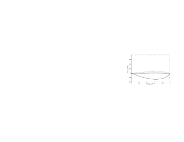
$\scriptstyle\mu=1\,\mathrm{GeV}$	$\scriptstyle\mu=500\,\mathrm{MeV}$

Figure 3: Contribution of the LLs to the normalized scalar form factor in a region where $F(s)$ is real. The solid, dotted, dashed and dashed-dotted lines denote the one–loop, two–loop, three–loop and four–loop LLs, respectively. The solid grey line indicates the tree–level result.

To illustrate the size of the LLs, we plot in Fig. 3 the numerical contributions of the LLs of the scalar form factor for two choices of the scale $\mu$. One sees that for $s>-0.85\,\mathrm{GeV}^{2}$, the LL corrections of higher–orders are always suppressed with respect to the lower orders.

5 Padé approximants

Padé approximants may be used to estimate higher–order terms. The Padé approximant $[M,N]$ for the scalar form factor is

$$[M,N]=\frac{\Xi_{M}}{\Xi_{N}}=\frac{F(s)}{F(0)}+O(p^{2(M+N)+2}),$$ (32)

where $\Xi_{K}$ only contains terms up to and including order $p^{2K}$. In Ref. [7], it is shown that the Padé approximant $[0,1]$ does not reproduce the correct factor of the two–loop LL. This shortcoming persists for the factors of the higher LL. Also the Padé approximants of the two– and three–loop LLs, $[1,1]$, $[0,2]$, $[2,1]$, $[1,2]$ and $[0,3]$, fail to reproduce the correct three– and four–loop LLs, respectively. In Tab. 1, we compare the two– and three–loop Padé approximants with the exact result.

Table 1: Padé approximants for the scalar form factor. Displayed are the exact and Padé values for the coefficients of the leading logarithms.

	$\frac{F(s)}{F(0)}$	$[0,1]$	$[1,1]$	$[0,2]$	$[2,1]$	$[1,2]$	$[0,3]$
$\frac{T_{3}}{N^{3}}$	$-\frac{143}{108}$	$-1$	$-\frac{1849}{1296}$	$-\frac{25}{18}$	$-\frac{143}{108}$	$-\frac{143}{108}$	$-\frac{143}{108}$
$\frac{T_{4}}{N^{4}}$	$\frac{15283}{9720}$	$1$	$\frac{79507}{46656}$	$\frac{2101}{1296}$	$\frac{20449}{13932}$	$\frac{1961}{1296}$	$\frac{1933}{1296}$

6 Summary and conclusion

1. In this letter, we study the structure of chiral logarithms in the two-flavour sector, in the chiral limit $m_{u}=m_{d}=0$. In particular, we investigate the chiral expansions of the scaler form factor of the pion, and of the correlator of two isoscalar quark currents. We confine our interest to the so called leading chiral logarithms, which are defined to be the ones accompanied with the least power of external momenta.

2. Standard techniques to calculate these logarithms – direct evaluation by calculating Feynman diagrams, or using renormalization group techniques – cannot be applied beyond three–loop accuracy, because the required labor becomes prohibitive.

3. We point out that, using unitarity and analyticity, the leading logarithms for the mentioned correlators can be calculated to any desired order with a modest calculational cost. We illustrate this claim with an evaluation of the leading logarithm for the scalar two–point function to five–loop order. As far as we are aware, this is the first evaluation of chiral logarithms at this accuracy. The numerical structure of the coefficients appears erratic to us.

4. The proposed technique makes use of Roy-equations for the $\pi\pi$ amplitude near threshold, in the chiral limit. While the Roy-kernels become singular in this limit, we argue (and explicitly check in one case) that these singularities do not affect the evaluation of the leading logarithms.

5. We compare our results with Padé approximants and confirm an earlier statement [7] concerning the use of this technique for the evaluation of chiral logarithms: knowledge of the coefficients up to and including those of order $N$ does not allow one to calculate the ones at order $N+1$ and higher.

7 Acknowledgements

It is a pleasure to thank G. Colangelo, C. Greub, H. Leutwyler, U.G. Meissner and all the members of the institute for informative discussions. We are indebted to J. Gasser for useful discussions and a careful reading of the manuscript. This work was supported in part by the Swiss National Science Foundation, by RTN, BBW-Contract No. 01.0357, and EC-contract HPRN-CT2002-00311 (EURIDICE).

Appendix A Roy equations

Using the integral representation for the kernels $K^{II^{\prime}}_{\ell\ell^{\prime}}(s,s^{\prime})$ given in [11] it is straightforward to calculate their imaginary parts,

$$\mbox{Im}\,K^{II^{\prime}}_{\ell\ell^{\prime}}(s,s^{\prime})=C_{su}^{II^{\prime}}\frac{4\ell^{\prime}+2}{s-4M_{\pi}^{2}}P_{\ell}\bigg{(}\frac{s+2s^{\prime}-4M_{\pi}^{2}}{4M_{\pi}^{2}-s}\bigg{)}P_{\ell^{\prime}}\bigg{(}\frac{2s+s^{\prime}-4M_{\pi}^{2}}{4M_{\pi}^{2}-s^{\prime}}\bigg{)},$$ (33)

where $C_{su}^{II^{\prime}}$ are the matrix elements of the crossing matrix $C_{su}$ and $P_{n}(x)$ are the Legendre polynomials. Note that it is crucial to use the projection interval $[0,1]$ in the integral representation of the kernels as given in [11]. Otherwise, the Roy equations cease to be valid for negative values of $s$.

Appendix B Suppression of higher intermediate states

In this appendix, we argue that intermediate states with more than two pions do not contribute to the leading logarithms of the scalar two–point function. In the sum

$$H(s+i\epsilon)-H(s-i\epsilon) = i\sum_{n}(2\pi)^{4}\delta^{(4)}(P_{n}-p)|\langle 0|S^{0}(0)|n\rangle|^{2}$$ (34)

appear the matrix elements of the $2k$ pion intermediate states

$$Y_{2k\pi}=\langle 0|S^{0}(0)|2k\pi\rangle.$$ (35)

The tree–level results of these matrix elements start with $F^{-2(k-1)}$. Because the integrand of the phase space integral is the modulus squared of $Y_{2k\pi}$, the lowest order contribution of the $2k$ pion intermediate states to the discontinuity of $H(s)$ is therefore of order $F^{-4(k-1)}$ and does not contain any logarithms. The loop corrections to these matrix elements are suppressed even stronger in $F^{-2}$. Take for example $k=2$. The four particle phase space integration would have to generate a logarithm squared to contribute to the leading term in the polynomial $P_{3}$. This is not possible and one way to see it is the following: Only diagrams with vertices solely from $\mathcal{L}_{2}$ contribute to the leading logarithms. The highest power of the pole term $\epsilon^{-1}$ is directly related to the highest power of the logarithm. Since the phase space integration in an infrared save theory does not produce a divergence, a phase space integration does not increase the power of the pole term and thus neither the power of a logarithm. In the case of the scalar form factor, the argument is the same. The higher intermediate states are also suppressed in $F^{-2}$.

References

- [1] S. Weinberg, PhysicaA 96 (1979) 327.
- [2] J. Gasser and H. Leutwyler, Annals Phys. 158 (1984) 142.
- [3] J. Bijnens, G. Colangelo and G. Ecker, Annals Phys. 280 (2000) 100 [arXiv:hep-ph/9907333].
- [4] J. Bijnens, G. Colangelo and G. Ecker, JHEP 9902 (1999) 020 [arXiv:hep-ph/9902437].
- [5] M. Buchler and G. Colangelo, Eur. Phys. J. C 32 (2003) 427 [arXiv:hep-ph/0309049].
- [6] M. Bissegger and A. Fuhrer, in preparation.
- [7] J. Gasser and U. G. Meissner, Nucl. Phys. B 357 (1991) 90.
- [8] J. Bijnens, G. Colangelo and P. Talavera, JHEP 9805 (1998) 014 [arXiv:hep-ph/9805389].
- [9] J. Bijnens, G. Colangelo, G. Ecker, J. Gasser and M. E. Sainio, Nucl. Phys. B 508 (1997) 263 [arXiv:hep-ph/9707291].
- [10] S. M. Roy, Phys. Lett. B 36 (1971) 353.
- [11] B. Ananthanarayan, G. Colangelo, J. Gasser and H. Leutwyler, Phys. Rept. 353 (2001) 207 [arXiv:hep-ph/0005297].