A Relativistic Flux-tube Model for Hybrid Mesons

Abstract

A number of authors have considered potential models for hybrid mesons. These frequently involve approximating the vibrating flux-tube by a set of beads, and making an adiabatic approximation which gives rise to a static inter-quark potential which has an effective repulsive $\frac{1}{r}$ potential. We show that this approximation is almost certainly wrong. Since the beads are presumably massless, the correct approximation requires the solution of a Klein-Gordon-like equation treating the beads and the quarks on the same footing. We show how to solve this in the one-bead case for massless quarks, and find the spectrum has an unexpected degeneracy. We generalise this to the $N_{B}$-bead case, which can still be solved exactly for massless quarks, and show how to renormalize the energy to obtain a plausible spectrum. We give a generic method to solve the equation for massive quarks, and use this to derive a different non-relativistic equation. The results show a smooth behaviour both with respect to the quark mass and the number of beads.

I Introduction

Many authors have considered models for hybrid mesons. In most cases, the method used is similar in spirit to the original work of Isgur and Paton Isgur and Paton (1985). In its simplest form, the meson is regarded as a $q\bar{q}$ state with an interaction potential produced by an oscillating string or flux-tube. A physical model for this consists of massive beads linked by a linear potential (Fig 1)

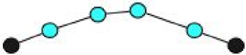
Figure 1: A hybrid meson model

These are treated non-relativistically in an adiabatic fashion and the oscillations are restricted to being perpendicular to the line joining the quarks. This basic idea has provided a rich source of models. There are justifications for various models from lattice-gauge theory (Bali (2000),Morningstar (2003),Allen et al. (1998)). More sophisticated analyses include non-adiabatic corrections Merlin and Paton (1985). and a number of phenomenological analyses: see e.g.(Swanson (2003), Close and Dudek (2004)). The work by Barnes, Close and Swanson Barnes et al. (1995) discusses a non-adiabatic model which has a similar starting point to the discussion below.

This paper discusses a formulation which escapes from some of these restrictions. Firstly we show how to eliminate the centre of mass from a N-bead non-relativistic model. We use this to examine the adiabatic approximation and show that it can lead to highly misleading results in a very simple case. Then we write down a model where both the quarks and beads are treated as Klein-Gordon particles. The resulting equation can be exactly solved in the case where both quarks and beads are massless, and we write down a variational expression for the case where the quarks are massive. There are a number of subtleties in this model and the spectrum has an unexpected form. We have not made an attempt to turn this into a realistic model for conventional and hybrid mesons.

II Centre of Mass diagonalization

The assumption that the quark motions are independent of the flux tube is not particularly logical for small quark mass. We therefore consider the extension of the flux-tube hybrid model to include the quarks. If we assume the quarks and the beads have small masses, we can write

$$\begin{array}[]{l}\mu_{n}=\frac{{m_{f}}}{N},n=2..N-1,\mu_{1}=m_{1}+\frac{{m_{f}}}{N},\mu_{N}=m_{N}+\frac{{m_{f}}}{N}\\ M=m_{f}+m_{1}+m_{N}\\ \end{array}$$

where the flux tube mass ${m_{f}}$ need not be a constant and we are allowing for the possibility of the quarks having different masses.

The full Schrödinger equations is

$$\left({\frac{1}{{2m_{1}}}\nabla_{1}^{2}+\frac{1}{{2m_{N}}}\nabla_{N}^{2}+\sum\limits_{k=2}^{N-1}{\frac{1}{{2m_{b}}}\nabla_{k}^{2}}+\sigma l_{N}\left({r,y_{n}}\right)}\right)\Psi=E\Psi$$

In the spirit of the adiabatic approximation, we could assume that the beads are restricted to oscillations perpendicular to the tube, so ${\nabla_{k}^{2}}$ is 2-D, but ${\nabla_{1}^{2}}$ and ${\nabla_{N}^{2}}$ are 3 dimensional, so the quarks can move in 3-D.

If the quarks are light, they need to be treated on the same footing as the beads, which means we must separate the centre-of-mass motion from the relative motion terms in the sum over the KE. The CoM given by

$$\vec{R}=\frac{{\mu\sum\limits_{n=2}^{N-1}{\vec{r}_{i}}+m_{1}\vec{r}_{1}+m_{N}\vec{r}_{N}}}{M}$$

Writing

$$\hat{r}_{1}=R=\frac{{\sum\limits_{n=1}^{N}{\mu_{i}\vec{r}_{i}}}}{M},\hat{r}_{i}=\vec{r}_{i}-\vec{r}_{i-1}(i\geq 2)$$ (1)

eliminates any cross terms of the form. $\frac{{\partial}}{{\partial R}}\frac{{\partial}}{{\partial\hat{r}_{i}}}$ Note that this reduces to the usual expression for the 2-body case. This can be inverted, via

$$\begin{array}[]{l}\vec{r}_{N}=R+\frac{{\mu_{1}\hat{r}_{2}}}{M}+\frac{{\left({\mu_{1}+\mu_{2}}\right)\hat{r}_{3}}}{M}+..+\frac{{\left({\mu_{1}+\mu_{2}+..\mu_{N-1}}\right)\hat{r}_{N}}}{M}\\ \vec{r}_{i-1}=\vec{r}_{i}-\hat{r}_{i}\\ \end{array}$$

This gives

$$\sum\limits_{n=1}^{N}{\frac{1}{{2\mu_{n}}}\nabla_{r_{n}}^{2}}=\frac{1}{{2M}}\nabla_{R}^{2}+\sum\limits_{n=1}^{N}{\frac{1}{{2\mu_{n}}}\left({\nabla_{\hat{r}_{n}}-\nabla_{\hat{r}_{n+1}}}\right)}^{2}$$

We now want to diagonalize the KE operator. Write

$$\sum\limits_{n=1}^{N}{\frac{1}{{2\mu_{n}}}\left({\nabla_{\hat{r}_{n}}-\nabla_{\hat{r}_{n+1}}}\right)}^{2}=\partial_{\bf{i}}^{\bf{T}}{\bf{G}}\partial_{\bf{i}}$$

where the matrix G is symmetric and tri-diagonal.

$${\bf{G}}=\left[{\begin{array}[]{*{20}c}{\frac{1}{{\mu_{1}}}+\frac{1}{{\mu_{2}}}}&{-\frac{1}{{\mu_{2}}}}&{}\hfil&{}\hfil\\ {-\frac{1}{{\mu_{2}}}}&{\frac{1}{{\mu_{2}}}+\frac{1}{{\mu_{3}}}}&{-\frac{1}{{\mu_{3}}}}&{}\hfil\\ {}\hfil&{-\frac{1}{{\mu_{3}}}}&{\frac{1}{{\mu_{3}}}+\frac{1}{{\mu_{4}}}}&{..}\\ {}\hfil&{}\hfil&{..}&{..}\\ \end{array}}\right]$$ (2)

We can then diagonalize this using

$${\bf{\hat{u}}}={\bf{S\hat{r}}},{\bf{S}}^{T}{\bf{GS}}=\Lambda$$

which allows the kinetic energy to be written

$$\frac{1}{{2m_{R}}}\frac{{\partial^{2}}}{{\partial r^{2}}}+\sum\limits_{n=1}^{N}{\frac{1}{{2\hat{\mu}_{n}}}\nabla_{u_{n}}^{2}}$$

It is then possible to solve the equation analytically if we make two further assumptions: that the motion is adiabatic, so that the beads oscillate perpendicular to the line joining the quarks and that P.E.

$$l_{N}\left({r,\hat{y}_{n}}\right)=\sigma\sum\limits_{i=1}^{N}{\left|{\hat{r}_{i}}\right|}=\sigma\sum\limits_{i=1}^{N}{\left[{\hat{y}_{i}^{2}+\left({\frac{r}{N}}\right)^{2}}\right]}^{1/2}$$

(where ${\hat{y}_{i}}$ is perpendicular to the line joining the quarks) can be expanded: i.e.

$$V_{N}\left({r,\hat{r}_{n}}\right)\approx r+\frac{N}{{2r}}\sum\limits_{i=1}^{N}{\hat{y}_{i}^{2}}$$

so the flux tube interaction gives rise to an oscillator, but with a strength that increases with N.

Since ${\bf{\hat{u}}}={\bf{S\hat{r}}}$ , the P.E. term can be written $\sum\limits_{i=1}^{N}{\left[{\hat{r}_{i}^{2}}\right]}=\sum\limits_{i=1}^{N}{\left[{\hat{u}_{i}^{2}}\right]}$ This allows the N-bead equations to be separated into N uncoupled equations, where the effective spring constant is given by

$$k_{eff}^{2}=\frac{{\sigma N}}{{\bar{r}}}$$

III Failure of the adiabatic method: Zero-bead case

We would like to check the validity of this expansion in a very simple example: the 0 bead case which be solved exactly in both 3-D and 2+1 D methods. The basic equation is

$$\left({\frac{{\hbar^{2}}}{{2m_{R}}}\nabla^{2}-\sigma r+E_{nl}}\right)\psi_{nl}\left({\vec{r}}\right)=0$$ (3)

III.0.1 Exact solution

As is well known, for l = 0, after conversion to a dimensionless form via

$$y=\beta\left({z-z_{n}}\right),z_{n}=\frac{{y_{n}}}{\beta},\beta=\left({\frac{{2m\sigma}}{{\hbar^{2}}}}\right)^{1/3}$$

one obtains the Airy equation giving

$$E_{n}=\left({\frac{{\hbar^{2}\sigma^{2}}}{{2m}}}\right)^{1/3}y_{n}$$

where $y_{n}$ is the n-th zero of the Airy function

III.0.2 Conventional Variational Solution

We can, of course, solve (3) by a standard variational approach with a Gaussian-wave function. The variational energy

$$E=\frac{{\hbar^{2}}}{{2m}}\beta^{2}\frac{3}{2}+\frac{{2\sigma}}{{\beta\sqrt{\pi}}}$$

gives

$$\beta={\rm{0}}{\rm{.867}}\left({\frac{{\sigma m}}{{\hbar^{2}}}}\right)^{1/3},E=1.865\left({\frac{{\hbar^{2}\sigma^{2}}}{m}}\right)^{1/3}$$

III.0.3 2+1-D solution:

We can now solve the 3-D equation by a “phonon” approx. This means put $\vec{r}=\left({x,\hat{y}}\right)$ so

$$\left|{\vec{r}}\right|=\sqrt{x^{2}+\hat{y}^{2}}\approx x+\frac{{\hat{y}^{2}}}{{2x}}$$

and the trial wave function is

$$\phi_{0}\left({x,\vec{r}}\right)=e^{-\left({\beta^{\prime\prime}x}\right)^{2}}e^{-\left({\beta^{\prime}\left(x\right)r}\right)^{2}}$$

The 2-D “phonon” equation has the form

$$\left({\frac{{\hbar^{2}}}{{2m_{R}}}\left({\frac{{\partial^{2}}}{{\partial y^{2}}}+\frac{1}{y}\frac{\partial}{{\partial r}}-\frac{{\ell^{2}}}{{y^{2}}}}\right)-\frac{{\sigma y^{2}}}{{2x}}+E_{nl}}\right)\psi_{nl}\left(r\right)=0$$

with the ground state solution

$$\beta^{\prime}=\frac{1}{\hbar}\sqrt{\frac{{\sigma m}}{x}},E^{\prime}\left(x\right)=\hbar\sqrt{\frac{\sigma}{{mx}}}$$

This then gives the corresponding 1-D equation

$$\left({\frac{{\hbar^{2}}}{{2m}}\frac{{\partial^{2}}}{{\partial x^{2}}}-\sigma x+\hbar\sqrt{\frac{\sigma}{{mx}}}+E}\right)\phi\left(x\right)=0$$

with a variational solution

$$E=\frac{{\hbar^{2}}}{{2m}}\frac{{\beta^{2}}}{2}+\frac{{g_{V}\sigma}}{{\sqrt{\pi}\beta}}+\frac{{\Gamma\left({\frac{1}{4}}\right)}}{{\sqrt{\pi}}}\left({\frac{\sigma}{m}}\right)^{1/2}\beta^{1/2}$$

which can be minimised numerically for $\beta$ and E.

III.0.4 Simultaneous minimisation

To justify a technique we will use later, we can minimise over both $\beta,\beta^{\prime}$ simultaneously. This means doing a non-linear minimisation for both the phonon and longitudinal modes: i.e. split the equation into transverse (phonon) and longitudinal motion as before

$$\begin{array}[]{l}\left({-\frac{{\hbar^{2}}}{{2m}}\left({\frac{{d^{2}}}{{dx^{2}}}+\frac{{\partial^{2}}}{{\partial y^{2}}}+\frac{1}{{y^{2}}}\frac{{\partial^{2}}}{{\partial\phi^{2}}}}\right)+\frac{1}{2}\sigma\sqrt{x^{2}+\hat{y}^{2}}}\right)\phi_{0}\left({x,\hat{y}}\right)\\ =E\phi_{0}\left({x,\hat{y}}\right)\\ \end{array}$$

and using a trial wave-function $\phi_{0}\left({x,\hat{y}}\right)=e^{-\left({\beta x}\right)^{2}/2}e^{-\left({\beta^{\prime}y}\right)^{2}/2}$ , perform simultaneous non-linear minimisation on $\beta,\beta^{\prime}$

III.0.5 Results

The results, using $m_{q}=300MeV,\sigma=180000MeV^{2}\$, are shown in table 1.

Table 1: Comparison of zero-bead results

	$\beta$	Energy
3-D exact	1.3203	1113.45
3-D variational	1.3850	1116.63
2+1-D phonon approximation	0.89668	1567.87
2+1-D minimization	1.3846	1116.62

We conclude that the phonon approximation is disastrously bad. It can be argued that the model is unrealistic, since the transverse motion could not be regarded as adiabatic in this case. However, we find similar results for a one-bead example, but there are no exact results to compare it.

IV Klein-Gordon Equation

The assumption that the quarks can be treated non-relativistically is not sensible when the quark mass is small. Further, it is hard to justify using a non-relativistic approximation in the limit that $N\to\infty$ since the bead mass goes to zero and the Schrödinger equation becomes meaningless. Hence we would like to have an equation which works for both massless beads and massless quarks.

We consider a Klein-Gordon equation for the both

$$\left({p_{i}^{2}c^{2}+m_{i}^{2}c^{4}}\right)\psi=0,m_{i}=\mu_{i}+\frac{{V_{i}}}{{c^{2}}}$$ (4)

where we have assumed that the confining potential transforms as a Lorentz scalar (assuming it transforms as the 4th component of a 4-vector leads to other problems: see Ram (1982)). Obviously a realistic model would require a Dirac equation for the quarks.

The spectrum should be well-behaved and independent of the mass in the $\mu_{0}\to 0$ limit, since the K-G equation becomes

$$\left({-\hbar^{2}\nabla^{2}-\frac{{E^{2}}}{{c^{2}}}+V^{2}}\right)\psi=0$$ (5)

We need to reduce the n-body K-G equation to a Schrödinger-like equation with no relative time. This does not appear to be in the literature. One cannot use a conventional reduced mass reduction: see (Ebert et al. (1998)).

If we have n particles with individual momenta $p_{i}$, we can obviously write the total momentum

$$P_{\mu}=\sum{p_{i\mu}}$$

which is correct relativistically or non-relativistically. Each bead or quark satisfies

$$\left({{\bf{p}}_{i}^{2}c^{2}+m_{i}^{2}c^{4}}\right)\psi=\varepsilon_{i}^{2}\psi,m_{i}=\mu+\frac{{V_{i}}}{{c^{2}}}$$

so by analogy with the preceding we write

$$p_{i}=\frac{{\varepsilon_{i}}}{E}P+\hat{q}_{i}-\hat{q}_{i-1}$$

Here and in what follows we use E to refer to total system energies and $\varepsilon$ to refer to individual component (quark, bead or phonon) energies. This is specified more carefully in Appendix A.

Then the ${\hat{q}}$’s can be reconstructed

$$\begin{array}[]{l}\hat{q}_{1}=p_{1}-\frac{{\varepsilon_{1}}}{E}P,\\ \hat{q}_{k}=p_{k}+\hat{q}_{k-1}-\frac{{\varepsilon_{k}}}{E}P=\sum\limits^{k}{p_{i}}-\frac{{\sum\limits^{k}{\varepsilon_{i}}}}{E}P\\ \end{array}$$

Note that $\hat{q}_{k}$ is still purely space-like: and the total energy $E=\sum\limits_{i=1}^{n}{\varepsilon_{i}}$ . Effectively in this process we are replacing the masses of the non-relativistic particles with the corresponding energies.

Hence

$$\sum\limits{\frac{{p_{i}^{2}}}{{E_{i}}}}=\frac{{P^{2}}}{E}+\sum\limits{\frac{{\left({\hat{q}_{i}-\hat{q}_{i-1}}\right)^{2}}}{{E_{i}}}}$$ (6)

so the overall K-G equation becomes

$$\begin{array}[]{l}\sum\limits{\frac{1}{{\varepsilon_{i}}}\left({p_{i}^{2}c^{2}+m_{i}^{2}c^{4}}\right)\Psi}\\ =\left({\frac{{P^{2}c^{2}}}{E}+\sum\limits{\frac{{\left({\hat{q}_{i}-\hat{q}_{i-1}}\right)^{2}c^{2}+\left({\mu_{i}c^{2}+V_{i}}\right)^{2}}}{{\varepsilon_{i}}}}}\right)\Psi=E\Psi\\ \end{array}$$ (7)

This equation is correct but apparently useless, since the individual ${\varepsilon_{i}}$ are unknown: in the equivalent NR treatment, the energies are replaced by masses whaich are, of course, known a priori. Below we show how to find the ${\varepsilon_{i}}$ by a variational trick.

V Massless quarks

We consider in turn the (trivial) zero-bead solution, the one bead solution and show how the solution can be generalised to the $N_{b}$-bead solution. Then we show how the $N_{b}$-bead solution can be renormalized to give a sensible spectrum. The starting assumption is that there is a scalar confining potential, $V=\sigma r$ equally divided between the quarks and the beads, so that (4) becomes

$$m_{i}^{2}c^{4}=\mu_{i}^{2}c^{4}+\mu_{i}\sigma rc^{2}+\frac{{\sigma^{2}r^{2}}}{4}\Rightarrow\frac{{\sigma^{2}r^{2}}}{4}$$

V.1 Massless zero-bead solution

The energy equations simplify to

$$E=Mc^{2},E_{R}=\frac{{Mc^{2}}}{2},\mu_{R}=\frac{M}{2},\varepsilon_{1}=\varepsilon_{2}=\frac{{Mc^{2}}}{2}$$

Then K-G eqn becomes

$$\left({-\frac{{4\hbar^{2}c^{2}}}{E}\nabla^{2}+\frac{{\sigma^{2}r^{2}}}{E}}\right)\psi=E\psi$$

with an immediate solution

$$\beta^{2}=\frac{\sigma}{{2\hbar c}},E^{2}=6\hbar c\sigma$$

V.2 Massless One-Bead

The interparticle potential becomes $V_{k}\left({\hat{r}_{n}}\right)=\frac{\sigma}{2}\left({\hat{r}_{k}+\hat{r}_{k-1}}\right)$. Hence the sum over potentials is

$$\begin{array}[]{l}V^{2}=\frac{{\sigma^{2}}}{4}\left({\frac{{\hat{r}_{1}^{2}}}{{\varepsilon_{1}}}+\frac{{\hat{r}_{1}^{2}+2\hat{r}_{2}\hat{r}_{1}+\hat{r}_{2}^{2}}}{{\varepsilon_{2}}}+\frac{{\hat{r}_{2}^{2}}}{{\varepsilon_{3}}}}\right)\\ =\frac{{\sigma^{2}}}{4}\left({\left({\hat{r}_{1}^{2}+\hat{r}_{2}^{2}}\right)\left({\frac{1}{{\varepsilon_{1}}}+\frac{1}{{\varepsilon_{2}}}}\right)+\frac{{2\hat{r}_{2}\hat{r}_{1}}}{{\varepsilon_{2}}}}\right)\\ \end{array}$$

giving

$$\left({-\hbar^{2}c^{2}\sum\limits_{i}{\frac{{\left({\nabla_{i}-\nabla_{i-1}}\right)^{2}}}{{\varepsilon_{i}}}}+V^{2}}\right)\psi=Mc^{2}\psi$$

The K.E. can be diagonalized with eigenvalues $1/\varepsilon_{+},1/\varepsilon_{-}$ given by

$$\begin{array}[]{l}E=2\varepsilon_{1}+\varepsilon_{2},\varepsilon_{+}=\varepsilon_{1},\varepsilon_{-}=\frac{{\varepsilon_{1}\varepsilon_{2}}}{{2\varepsilon_{1}+\varepsilon_{2}}}=\frac{{\varepsilon_{1}\varepsilon_{2}}}{E},\\ \frac{1}{{\varepsilon_{1}}}+\frac{1}{{\varepsilon_{2}}}=\frac{1}{2}\left({\frac{1}{{\varepsilon_{+}}}+\frac{1}{{\varepsilon_{-}}}}\right)\\ \hat{u}_{\pm}=\frac{1}{{\sqrt{2}}}\left({\hat{r}_{1}\pm\hat{r}_{2}}\right),\hat{r}_{1}^{2}+\hat{r}_{2}^{2}=\hat{u}_{+}^{2}+\hat{u}_{-}^{2}\\ 2\hat{r}_{2}\hat{r}_{1}=\left({\hat{u}_{+}^{2}-\hat{u}_{-}^{2}}\right)\\ \end{array}$$

(note that this is just the relativistic analog of the result in Merlin and Paton Merlin and Paton (1985). Hence the K-G equation becomes

$$\left({-\hbar^{2}c^{2}\left({\frac{{\nabla_{+}^{2}}}{{\varepsilon_{+}}}+\frac{{\nabla_{-}^{2}}}{{\varepsilon_{-}}}}\right)+\frac{{\sigma^{2}}}{4}\left[{\hat{u}_{+}^{2}\frac{1}{{\varepsilon_{-}}}+\hat{u}_{-}^{2}\frac{1}{{\varepsilon_{+}}}}\right]}\right)\psi=E\psi$$

which separates into two phonon equations:

$$\left({-\frac{{\hbar^{2}c^{2}}}{{\varepsilon_{\pm}}}\nabla_{\pm}^{2}+\frac{{\sigma^{2}}}{{4\varepsilon_{\mp}}}\hat{u}_{\pm}^{2}}\right)\psi=\hat{\varepsilon}_{\pm}\psi$$

Note the distinction between the $\varepsilon_{i}$ (individual energies of the quarks and bead) and $\hat{\varepsilon}_{\pm}$ (individual energies of the phonon states). This has obvious solutions:

$$\begin{array}[]{l}\beta_{\pm}^{2}=\frac{\sigma}{{2c\hbar}}\left({\frac{{\varepsilon_{\pm}}}{{\varepsilon_{\mp}}}}\right)^{1/2},\hat{\varepsilon}_{\pm}=\frac{{c\hbar\sigma}}{{2\sqrt{\varepsilon_{+}\varepsilon_{-}}}}\left({2n_{\pm}+l_{\div}+\frac{3}{2}}\right),\\ E_{0}=\hat{\varepsilon}_{+}+\hat{\varepsilon}_{-}=\varepsilon_{+}+\varepsilon_{-}=\frac{{3c\hbar\sigma}}{{4\sqrt{\varepsilon_{+}\varepsilon_{-}}}}\\ \end{array}$$

To solve this, we will assume that the quarks carry fractions $\alpha_{1}$ of the total energy of the system, and regard $\alpha_{1}$ as a variational parameter, so

$$\begin{array}[]{l}\varepsilon_{1}=\alpha_{1}E=\varepsilon_{3}=\varepsilon_{+},\varepsilon_{2}=\alpha_{B}E,\alpha_{B}=(1-2\alpha_{1})\\ \varepsilon_{-}=\alpha_{1}\alpha_{B}E\Rightarrow E^{2}\left({\alpha_{1}}\right)=\frac{{3c\hbar\sigma}}{{\sqrt{\alpha_{1}^{2}(1-2\alpha_{1})}}}\\ \end{array}$$

gives a minimum value of $\alpha_{1}=1/3$: i.e. the quarks and the bead carry an equal fraction of the energy, which is what we expect. This gives

$$\beta_{+}^{2}=\frac{\sigma}{{2c\hbar}}\left({\frac{1}{3}}\right)^{1/2},\beta_{-}^{2}=\frac{\sigma}{{2c\hbar}}\left(3\right)^{1/2},E^{2}=\frac{3}{2}\sqrt{27}c\hbar\sigma$$

Physically we can interpret the two solutions as show in fig 2: the + solution corresponds to the two quarks moving in opposite direction while the bead remains stationary at the centre of mass, while the - solution corresponds to the quarks moving in the same direction but opposite to the bead.

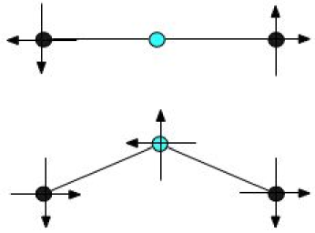
Figure 2: Two modes for one-bead model

It is worth noting the peculiar feature of the solution: the two phonon states have the same excitation spectrum but different $\beta$’s.

V.3 Massless n-bead solution

The overall K-G equation (7) becomes

$$\left({\sum\limits{\frac{{\left({\hat{q}_{i}-\hat{q}_{i-1}}\right)^{2}c^{2}}}{{E_{i}}}}+\frac{{\sigma^{2}}}{4}\sum\limits{\frac{{\left({\hat{r}_{i}+\hat{r}_{i-1}}\right)^{2}}}{{E_{i}}}}}\right)\Psi=E\Psi$$

If we assume that the ${\varepsilon_{i}}$’s are equal

$$\varepsilon_{i}=\frac{E}{N+1}$$ (8)

then this can be solved (we justify the assumption below). The previous method generalises:

$$\begin{array}[]{l}\left({-\frac{{\hbar^{2}c^{2}N}}{E}\sum\limits{\left({\nabla_{i}-\nabla_{i-1}}\right)^{2}}+\frac{N}{E}\frac{{\sigma^{2}}}{4}\sum\limits{\left({\hat{r}_{i}+\hat{r}_{i-1}}\right)^{2}}}\right)\psi=\\ \left({-\frac{{\hbar^{2}c^{2}N}}{E}\sum\limits{\nabla_{i}G_{ij}\nabla_{j}}+\frac{N}{E}\frac{{\sigma^{2}}}{4}\sum\limits{\hat{r}_{i}G^{\prime}_{ij}\hat{r}_{j}}}\right)\psi=E\psi\\ \end{array}$$

where

$$G=\left[{\begin{array}[]{*{20}c}2&{-1}&{}\hfil&{}\hfil\\ {-1}&2&{-1}&{}\hfil\\ {}\hfil&{-1}&2&{-1}\\ {}\hfil&{}\hfil&{-1}&2\\ \end{array}}\right],G^{\prime}=\left[{\begin{array}[]{*{20}c}2&1&{}\hfil&{}\hfil\\ 1&2&1&{}\hfil\\ {}\hfil&1&2&1\\ {}\hfil&{}\hfil&1&2\\ \end{array}}\right]$$

and

$$\hat{u}={\bf{S}}\hat{r},{\bf{S}}^{T}{\bf{GS}}=\Lambda$$ (9)

The structure is obviously similar to (2).

The KE term can be diagonalized as before. The same operation that digaonalizes G also diagonalizes $G^{\prime}$. The eigenvalues are given by Yueh (2005), .

$$\Lambda_{N}^{i}=\left({2\sin\left({\frac{{\pi i}}{{2\left({N+1}\right)}}}\right)}\right)^{2}$$

This then separates to give a set of N uncoupled “phonon” equations of the form

$$\left({-\frac{{\hbar^{2}c^{2}N}}{E}\Lambda_{i}^{N}\nabla_{u_{i}}^{2}+\frac{N}{E}\frac{{\sigma^{2}}}{4}\Lambda_{N-i}^{N}\hat{u}_{i}^{2}}\right)\psi=\hat{\varepsilon}_{i}\psi$$

which have the usual SHO form, with different interpretations of the energy and potential. With a modification of the usual substitutions

$$\begin{array}[]{l}\left({\beta_{i}^{N}}\right)^{2}=\sqrt{\frac{{\Lambda_{N-i}}}{{\Lambda_{i}}}}\frac{\sigma}{{2\hbar}}=\cot\left({\frac{{\pi i}}{{N+1}}}\right)\frac{\sigma}{{2\hbar}}\\ \hat{\varepsilon}^{N}_{i}=\frac{{c\hbar\sigma\left({N+1}\right)}}{{2E^{N}}}\left({2n_{i}+l_{i}+\frac{3}{2}}\right)\sqrt{\Lambda_{i}\Lambda_{N-i}}\\ =\frac{{c\hbar\sigma\left({N+1}\right)}}{{2E^{N}}}\left({2n_{i}+l_{i}+\frac{3}{2}}\right)\sin\left({\frac{{\pi i}}{{N+1}}}\right)\\ \end{array}$$ (10)

we can write the solution as

$$\psi\left({\hat{r}_{i}}\right)=A\zeta_{i}^{l}L_{n_{i}}^{l}\left({\zeta_{i}^{2}}\right)e^{-\zeta_{i}^{2}},\zeta_{i}=\beta_{i}\hat{u}_{i}$$

The energies can be summed to give the total energy

$$\begin{array}[]{l}E^{N}=\sum\limits_{i=1}^{N}{\hat{\varepsilon}_{i}^{N}}=\frac{3}{2}\frac{{c\hbar\sigma\left({N+1}\right)}}{{2E^{N}}}\sum\limits_{i=1}^{N}{\sin\left({\frac{{\pi i}}{{N+1}}}\right)=}\\ =\frac{3}{2}\frac{{c\hbar\sigma\left({N+1}\right)}}{{2E^{N}}}\frac{{\sin\left({\frac{\pi}{{N+1}}}\right)}}{{1-\cos\left({\frac{\pi}{{N+1}}}\right)}}\\ \end{array}$$

so

$$\left({E^{N}}\right)^{2}\approx\frac{3}{2}\frac{{c\hbar\sigma}}{{\pi E^{N}}}\left({N+1}\right)^{2}$$

There are several problems with this solution. Not surprisingly, the total energy is divergent as $N\to\infty$. Secondly the curious degeneracy noted above remains: the energy of the $n^{th}$ and $(N-n)^{th}$ levels are equal, even though they are described by different values of $\beta$. This violates one’s intuitive idea that large $\beta$ corresponds to small E and vice-versa. Finally, the individual energies of the phonon modes are

$$\hat{\varepsilon}^{N}_{i}\approx\sqrt{\frac{{3c\hbar\sigma}}{2}}\frac{{\pi^{1/2}}}{2}\sin\left({\frac{{\pi i}}{{N+1}}}\right)\approx\sqrt{\frac{{3c\hbar\sigma}}{2}}\frac{{\pi^{3/2}i}}{{2\left({N+1}\right)}}$$

so the excitation energies are vanishingly small in the $N\to\infty$ limit.

V.4 Energy Renormalization

In order to obtain finite answers, we subtract a energy $\Delta E^{N}$ from the total non-renormalized energy $E^{N}$ given by (10) to give a (fixed) renormalized energy $\tilde{E}^{0}$ for the ground state:

$$\tilde{E}^{0}=E^{N}-\Delta E^{N}$$

By writing

$$\Delta E^{N}=\sum\limits_{i=1}^{N}{\hat{\varepsilon}_{i}^{N}\left({0,0}\right)}-\tilde{E}^{0}$$

gives the renormalized energy of each phonon mode as

$$\tilde{\varepsilon}^{N}_{i}\left({n_{i},l_{i}}\right)=\frac{{c\hbar\sigma\left({N+1}\right)}}{{2\tilde{E}^{0}}}\left({2n_{i}+l_{i}}\right)\sin\left({\frac{{\pi i}}{{N+1}}}\right)$$ (11)

This now has a sensible limit for all modes in the $N\to\infty$ limit

$$\tilde{\varepsilon}^{\infty}_{i}\left({n_{i},l_{i}}\right)=\frac{{c\hbar\sigma}}{{2\tilde{E}^{0}}}\left({2n_{i}+l_{i}}\right)\pi i$$

It makes sense to have the energy fixed by the zero-bead solution, so

$$\tilde{E}^{0}=\sqrt{6\hbar c\sigma}$$ (12)

and the total energy of the excited phonon states is then given (in the $N\to\infty$ limit) by

$$E^{\infty}\left({n_{k},l_{k}}\right)=\sqrt{6c\hbar\sigma}\left({1+\frac{\pi}{{12}}\sum\limits{\left({2n_{i}+l_{i}}\right)i}}\right)$$ (13)

VI Massive quarks

We have ignored the quark masses: this introduces two extra types of term, via

$$m_{i}^{2}c^{4}=\mu_{i}^{2}c^{4}+\mu_{i}\sigma rc^{2}+\frac{{\sigma^{2}r^{2}}}{4}$$

The second term, in particular, causes considerable trouble since it mixes the phonon states. We provide a very rapid numerical algorithm for taking this into account. In principle one can include a bead-mass: there is no need to do so, and we show that one can in fact find a non-relativistic reduction of the equation even with a massless bead. Again, we analyse the 0-bead, 1-bead and n-bead solutions.

VI.1 Massive quarks, zero-bead case

We consider the general unequal-mass case. The K-G equation is

$$\left({-\frac{{\hbar^{2}c^{2}}}{{\varepsilon_{R}}}\nabla^{2}+\frac{1}{{\varepsilon_{1}}}\left({\mu_{1}^{2}c^{4}+\mu_{1}c^{2}\sigma r+\frac{1}{4}\sigma^{2}r^{2}}\right)+\frac{1}{{\varepsilon_{2}}}\left({\mu_{2}^{2}c^{4}+\mu_{2}c^{2}\sigma r+\frac{1}{4}\sigma^{2}r^{2}}\right)}\right)\psi=E\psi$$

In order to solve all of this variationally (and to connect this easy example with later equations), we proceed as follows.

1. Assume that the quarks carry fractions $\alpha_{1}$, $\alpha_{2}$ of the total energy of the system. Then

   $$\varepsilon_{1}=\alpha_{1}E,\varepsilon_{2}=\alpha_{2}E,\varepsilon_{R}=\alpha_{1}\alpha_{2}E,\alpha_{1}+\alpha_{2}=1$$

   obviously $0<\alpha_{1},\alpha_{2}<1$

2. Hence the K-G equation becomes

   $$\begin{array}[]{l}\left({-\frac{{\hbar^{2}c^{2}}}{{\alpha_{1}\alpha_{2}}}\nabla^{2}+\frac{{\mu_{1}^{2}c^{4}}}{{\alpha_{1}}}+\frac{{\mu_{2}^{2}c^{4}}}{{\alpha_{2}}}+c^{2}\sigma r\left({\frac{{\mu_{1}}}{{\alpha_{1}}}+\frac{{\mu_{2}}}{{\alpha_{2}}}}\right)+\frac{{\sigma^{2}r^{2}}}{{4\alpha_{1}\alpha_{2}}}}\right)\psi\\ =E^{2}\psi\\ \end{array}$$ (14)

3. Use a Gaussian trial wave-function, as suggested by the massless case, giving the variational energy:

   $$\begin{array}[]{l}E^{2}=\frac{{\hbar^{2}c^{2}}}{{\alpha_{1}\alpha_{2}}}\frac{3}{2}\beta^{2}+\frac{{\mu_{1}^{2}c^{4}}}{{\alpha_{1}}}+\frac{{\mu_{2}^{2}c^{4}}}{{\alpha_{2}}}+\\ c^{2}\sigma\left({\frac{{\mu_{1}}}{{\alpha_{1}}}+\frac{{\mu_{2}}}{{\alpha_{2}}}}\right)\frac{2}{{\beta\sqrt{\pi}}}+\frac{{\sigma^{2}}}{4}\frac{3}{{2\alpha_{1}\alpha_{2}\beta^{2}}}\\ \end{array}$$ (15)

This obviously contains the massless case.

VI.1.1 Non-relativistic Reduction

It is not obvious that this technique gives a sensible non-relativistic reduction. If the masses are large and equal, $M=2\mu+\frac{{E_{B}}}{{c^{2}}}$ where $E_{B}$ is the binding energy. Putting

$$\begin{array}[]{l}E=Mc^{2}=\mu_{1}c^{2}+\mu_{2}c^{2}+E_{B},\\ \varepsilon_{1}\approx\mu_{1}c^{2},\varepsilon_{2}\approx\mu_{2}c^{2},\varepsilon_{R}\approx\frac{{\mu_{1}\mu_{2}c^{2}}}{{\mu_{1}+\mu_{2}}}=\mu_{R}c^{2}\\ \end{array}$$

Ignoring terms with $V^{2},E_{B}^{2}$ in (14) gives

$$\left({-\frac{{\hbar^{2}}}{{2\mu_{R}}}\nabla^{2}+\sigma r-E_{B}}\right)\psi=0$$

which is the Schrodinger equation.

However, we wish to use a variational method, and it is not conventional to find the reduced mass by this technique! We get a mass term from (15) of the form $\alpha_{1}\alpha_{2}\left({\frac{{\mu_{1}^{2}c^{4}}}{{\alpha_{1}}}+\frac{{\mu_{2}^{2}c^{4}}}{{\alpha_{2}}}-E^{2}}\right)$. In the infinite mass limit, this gives an apparent mass term

$$\begin{array}[]{l}\hat{m}^{2}=\left({\mu_{1}^{2}\left({1-\alpha_{1}}\right)^{2}+\mu_{2}^{2}\alpha_{1}^{2}-2\mu_{1}\left({1-\alpha_{1}}\right)\mu_{2}\alpha_{1}}\right)\\ =\left({\mu_{1}\left({1-\alpha_{1}}\right)-\mu_{2}\alpha_{1}}\right)^{2}\\ \end{array}$$

Minimising this gives (obviously) $\alpha_{1}=\frac{{\mu_{1}}}{{\mu_{1}+\mu_{2}}}$ so the “reduced energy” becomes

$$\varepsilon_{R}=\alpha_{1}\alpha_{2}E=\mu_{R}c^{2}$$

as expected.

VI.1.2 Coulomb-interaction and non-zero angular momentum

We can generalise this by including a Coulomb-type interaction (see Olsson Olsson (1997)) $V(r)=\frac{\kappa}{r}$ which is the fourth component of a 4-vector, so that

$$\varepsilon_{1}^{2}\to\left({\varepsilon_{1}-\frac{\kappa}{{2r}}}\right)^{2}=\varepsilon_{1}\left({\varepsilon_{1}-\frac{\kappa}{r}+\frac{{\kappa^{2}}}{{\varepsilon_{1}4r^{2}}}}\right)$$

This adds a term

$$-\frac{{2\kappa E}}{r}+\frac{{\kappa^{2}}}{{4\alpha_{1}\alpha_{2}r^{2}}}$$

to the K-G equation.

We can also generalise this to any angular momentum $\ell$: both these generalisations require us to use a modified trial wave function of the form

$$\psi\left(r\right)=Cr^{p}e^{-\frac{{\beta^{2}r^{2}}}{2}}$$

We will write the variational energy in the generic form

$$\begin{array}[]{l}E^{2}\left({\mu_{1},\mu_{2},\ell}\right)=\hbar^{2}c^{2}d_{-2}\left({\alpha_{i}}\right)\beta^{2}+\kappa Ed_{-1}\left(\beta\right)+\\ c^{4}d_{0}\left({\mu_{j},\alpha_{i}}\right)+\sigma c^{2}d_{1}\left(\beta\right)+\frac{{\sigma^{2}}}{4}\frac{{d_{2}^{k}\left({\alpha_{i}}\right)}}{{\beta^{2}}}\\ \end{array}$$

where

$$\begin{array}[]{l}d_{-2}=\frac{1}{{\left({p+\frac{1}{2}}\right)}}\left({\frac{{4l\left({l+1}\right)+4p+3}}{{2\alpha_{1}\alpha_{2}}}+\frac{{\kappa^{2}}}{4}}\right)\\ d_{-1}=2\beta\frac{{\Gamma\left({p+1}\right)}}{{\Gamma\left({p+\frac{3}{2}}\right)}}\\ d_{0}=\frac{{\mu_{1}^{2}}}{{\alpha_{1}}}+\frac{{\mu_{2}^{2}}}{{\alpha_{2}}}\\ d_{1}=\left({\frac{{\mu_{1}}}{{\alpha_{1}}}+\frac{{\mu_{1}}}{{\alpha_{2}}}}\right)\frac{{\Gamma\left({p+2}\right)}}{{\beta\Gamma\left({p+\frac{3}{2}}\right)}}\\ d_{2}=\frac{1}{4}\left({p+\frac{3}{2}}\right)\\ \end{array}$$ (16)

This generic form is useful since it generalises to the one-bead and n-bead case, and it can be solved by a rapid algorithm which is outlined in appendix B. For the purposes of renormalizing the n-bead energy later, we regard the zero-bead energy as the renormalized energy of the ground state

$$\tilde{E}^{0}=E\left({\mu_{1},\mu_{2},\ell}\right)$$

in the sense of (12).

VI.2 Massive quarks: one-bead

To solve the unequal-mass one-bead case, we will assume that the quarks carry fractions $\alpha_{1}$, $\alpha_{3}$ of the total energy of the system.

$$\varepsilon_{1}=\alpha_{1}E,\varepsilon_{2}=\alpha_{B}E,\varepsilon_{3}=\alpha_{3}E,\alpha_{B}=(1-\alpha_{1}-\alpha_{3})$$

This introduces two extra terms. There is a constant term with same

$$d_{0}=\frac{{\mu_{1}^{2}c^{4}}}{{\alpha_{1}}}+\frac{{\mu_{2}^{2}c^{4}}}{{\alpha_{2}}}$$ (17)

as in (16). The second term is

$$2c^{2}\left({\frac{{\mu_{1}V_{1}}}{{\varepsilon_{1}}}+\frac{{\mu_{N}V_{N}}}{{\varepsilon_{3}}}}\right)=c^{2}\frac{\sigma}{E}\left({\frac{{\mu_{1}\left|{\hat{r}_{1}}\right|}}{{\alpha_{1}}}+\frac{{\mu_{N}\left|{\hat{r}_{2}}\right|}}{{\alpha_{3}}}}\right)$$ (18)

is more difficult to handle

In the equal mass case, (17) becomes:

$$d_{0}=2\frac{{\mu_{1}^{2}}}{{\alpha}}$$

and the linear term (18) becomes

$$\sqrt{2}\frac{{\mu\sigma}}{{\alpha_{1}E}}\left|{\hat{u}_{+}^{2}+\hat{u}_{-}^{2}}\right|^{1/2}\left({1+O\left({\cos^{2}\left(\theta\right)}\right)+...}\right)$$

Ignoring the higher order terms gives

$$\frac{1}{{\alpha_{1}E}}\left(\begin{array}[]{l}-\hbar^{2}c^{2}\left({\nabla_{+}^{2}+\frac{{\nabla_{-}^{2}}}{{\alpha_{B}}}}\right)+2\mu^{2}c^{4}+\\ \sqrt{2}c^{2}\mu\sigma\left|{\hat{u}_{+}^{2}+\hat{u}_{-}^{2}}\right|^{1/2}+\frac{{\sigma^{2}}}{4}\left[{\frac{{\hat{u}_{+}^{2}}}{{\alpha_{B}}}+\hat{u}_{-}^{2}}\right]\\ \end{array}\right)\psi=E\psi$$

The linear term (18) gives us a new term in the variational energy

$$\begin{array}[]{l}A^{2}\sqrt{2}c^{2}\frac{{\mu\sigma}}{{E_{1}}}\int{\int{e^{-\beta_{+}^{2}u_{+}^{2}}e^{-\beta_{-}^{2}u_{-}^{2}}\left|{\hat{u}_{+}^{2}+\hat{u}_{-}^{2}}\right|^{1/2}u_{+}^{2}u_{-}^{2}du_{+}du_{-}}}\\ =\sqrt{2}c^{2}\frac{{\mu\sigma}}{{\alpha_{1}E}}f_{00}^{1}\left({\beta_{+},\beta_{-}}\right)\\ \end{array}$$

which can be written as $d_{1}\left({\alpha,\beta}\right)=\sqrt{2}c^{2}\frac{{\mu\sigma}}{{\alpha E}}f_{00}^{1}\left({\beta_{+},\beta_{-}}\right)$ in the notation of (16). We show how to evaluate $f_{00}^{1}$ in Appendix C. . Hence the overall variational solution becomes

$$\begin{array}[]{l}E^{2}=\frac{3}{2}\frac{{\hbar^{2}c^{2}}}{{\alpha_{1}}}\left({\beta_{+}^{2}+\frac{{\beta_{-}^{2}}}{{\alpha_{1}\alpha_{B}}}}\right)+2\mu^{2}c^{4}+\\ \sqrt{2}c^{2}\frac{{\mu\sigma}}{{\alpha_{1}}}f_{00}^{1}\left({\beta_{+},\beta_{-}}\right)+\frac{{3\sigma^{2}}}{{8\alpha_{1}}}\left({\frac{1}{{\alpha_{B}\beta_{+}^{2}}}+\frac{1}{{\beta_{-}^{2}}}}\right)\\ \end{array}$$

which can be rapidly solved by the technique of Appendix A.

VI.2.1 Non-relativistic reduction

It is useful to have a non-relativistic reduction of this equation. The conventional reduction of allowing the bead and quark masses to become large will not work, since we believe the bead mass is zero.. We need to reduce (VI.2) to a corresponding NR equation for comparison. Putting $E=2\mu c^{2}+E_{B}$ gives

$$\begin{array}[]{l}\alpha_{1}E^{2}-2\mu^{2}c^{4}\approx 2\mu^{2}c^{4}\left({2\alpha_{1}-1}\right)+4\alpha_{1}\mu c^{2}E_{B}\\ =4\alpha_{1}\mu c^{2}E_{B}-2\mu^{2}c^{4}\alpha_{B}\\ \end{array}$$

The K-G equation then becomes

$$\begin{array}[]{l}\frac{1}{{\alpha_{1}}}\left({-\frac{{\hbar^{2}}}{{4\mu}}\left({\nabla_{+}^{2}+\frac{{\nabla_{-}^{2}}}{{\alpha_{B}}}}\right)+\frac{1}{2}\mu c^{2}\alpha_{B}+\frac{1}{{2\sqrt{2}}}\sigma\left|{\hat{u}_{+}^{2}+\hat{u}_{-}^{2}}\right|^{1/2}}\right)\psi\\ =E_{B}\psi\\ \end{array}$$

so the bead has acquired a pseudo-mass $\alpha_{1}\alpha_{B}\mu$

This has the variational solution

$$\begin{array}[]{l}E_{B}=\frac{3}{2}\frac{{\hbar^{2}}}{{4\mu}}\left({\frac{{\beta_{+}^{2}}}{{\alpha_{1}}}+\frac{{\beta_{-}^{2}}}{{\alpha_{B}\alpha_{1}}}}\right)+\\ \frac{1}{{2\sqrt{2}\alpha_{1}}}\sigma f_{00}^{1}\left({\beta_{+},\beta_{-}}\right)+\frac{1}{2}\mu c^{2}\frac{{\alpha_{B}}}{{\alpha_{1}}}\\ \end{array}$$

Note that the masslessness of the bead does not give rise to a Schrödinger equation with zero mass. The usual limit of $\alpha=1/2$ which would minimise the mass term does not minimise the energy.

VI.3 Massive Quarks: n-bead case

We want $N_{B}=N-2$ beads and 2 quarks, with different masses, so that we have N particles in all and the quarks have a fraction $\alpha_{1},\alpha_{N}$ of the total energy, so each bead has a fraction

$$\alpha_{B}=\frac{{1-\alpha_{1}-\alpha_{2}}}{{N-2}}$$ (19)

of the total. Now the K-G eqn becomes

$$\sum\limits{\frac{{-\hbar^{2}\left({\nabla_{i}-\nabla_{i-1}}\right)^{2}c^{2}+\left({\mu_{i}c^{2}+V_{i}}\right)^{2}}}{{E_{i}}}}\Psi=E\Psi$$

The KE and $V^{2}$ terms give expressions similar to (2) with G and $G^{\prime}$ are now given by

$$\begin{array}[]{l}G=\left[{\begin{array}[]{*{20}c}{\alpha_{1}^{\prime}+1}&{-1}&{}\hfil&{}\hfil&{}\hfil\\ {-1}&2&{-1}&{}\hfil&{}\hfil\\ {}\hfil&{-1}&2&{-1}&{...}\\ {}\hfil&{...}&{...}&{..}&{..}\\ {}\hfil&{}\hfil&{}\hfil&{-1}&{\alpha_{2}^{\prime}+1}\\ \end{array}}\right]\\ G^{\prime}=\left[{\begin{array}[]{*{20}c}{\alpha_{1}^{\prime}+1}&1&{}\hfil&{}\hfil&{}\hfil\\ 1&2&1&{}\hfil&{}\hfil\\ {}\hfil&1&2&1&{...}\\ {}\hfil&{...}&{...}&{..}&{..}\\ {}\hfil&{}\hfil&{}\hfil&1&{\alpha_{2}^{\prime}+1}\\ \end{array}}\right]\\ \end{array}$$

with

$$\alpha_{1}^{\prime}=\frac{{1-\alpha_{1}-\alpha_{N}}}{{\alpha_{1}\left({N-2}\right)}}=\frac{{\alpha_{B}}}{{\alpha_{1}}}$$

The term in $\mu V$ becomes

$$2c^{2}\left({\frac{{\mu_{1}V_{1}}}{{\varepsilon_{1}}}+\frac{{\mu_{N}V_{N}}}{{\varepsilon_{N}}}}\right)=\frac{{\sigma c^{2}}}{E}\left({\frac{{\mu_{1}\left|{\hat{r}_{1}}\right|}}{{\alpha_{1}}}+\frac{{\mu_{N}\left|{\hat{r}_{N}}\right|}}{{\alpha_{N}}}}\right)$$

Finally the mass term gives

$$c^{4}\left({\frac{{\mu_{1}^{2}}}{{\varepsilon_{1}}}+\frac{{\mu_{N}^{2}}}{{\varepsilon_{N}}}}\right)=\frac{{c^{4}}}{E}\left({\frac{{\mu_{1}^{2}}}{{\alpha_{1}}}+\frac{{\mu_{1}^{2}}}{{\alpha_{N}}}}\right)$$

as before. There are several new difficulties:

1. for non-equal masses, diagonalizing the KE matrix does not diagonalize the PE matrix.

2. the linear terms like ${\mu_{1}\left|{\hat{r}_{1}}\right|}$ involve all the $\hat{u}_{i}$’s, so the $\mu V$ is very complex.

3. there are $(N_{b}+1)$ different $\beta$’s (one for each phonon mode) which must be found variationally.

4. in addition, we have $\alpha_{1}$ and $\alpha_{N}$ which must be regarded as variational parameters.

Surprisingly, this can be approximately solved by a quite simple numerical technique: the algorithm is as follows.

1. Guess $\alpha_{1},\alpha_{N}$

2. Diagonalize G and find eigenvectors $e_{i}^{j}$

3. Ignore off-diagonal terms in ${\bf{e}}^{\bf{T}}{\bf{G^{\prime}e}}=\Lambda^{\prime}$

4. Write $\hat{r}_{1}=\sum\limits{e_{j}^{\left(1\right)}u_{j}}$ so that

   $$\left|{\hat{r}_{1}}\right|=\sqrt{\hat{r}_{1}^{2}}=\sqrt{\sum\limits{e_{j}^{\left(1\right)}e_{k}^{\left(1\right)}u_{j}u_{k}}}$$

5. Then (approximately) the expectation values required for the linear interaction can be found (See Appendix D):

   $$f_{1}\left({\beta_{i}}\right)=\left\langle{\left|{\hat{r}_{1}}\right|}\right\rangle\approx\left({\sum\limits_{i=1}^{N}{\left({l_{i}+\frac{3}{2}}\right)\left({\frac{{e_{i}^{\left(1\right)}}}{{\beta_{i}}}}\right)^{2}}}\right)^{1/2}$$

6. This gives us a total (non-renormalized) energy of the form:

   $$\begin{array}[]{l}E^{2}=\hbar^{2}c^{2}\sum\limits_{j}{\Lambda_{j}\beta_{j}^{2}\left({l_{j}+\frac{3}{2}}\right)}+\frac{{\mu_{1}^{2}c^{4}}}{{\alpha_{1}}}+\frac{{\mu_{1}^{2}c^{4}}}{{\alpha_{N}}}\\ 2\sigma c^{2}\left({\frac{{\mu_{1}}}{{\alpha_{1}}}f_{1}\left({\beta_{i}}\right)+\frac{{\mu_{N}}}{{\alpha_{N}}}f_{N}\left({\beta_{i}}\right)}\right)+\frac{{\sigma^{2}}}{4}\sum\limits{\frac{{\Lambda_{j}^{\prime}}}{{\beta_{j}^{2}}}\left({l_{j}+\frac{3}{2}}\right)}\\ \end{array}$$

   to be minimised to find the $\beta_{j}$. Obviously if $\mu_{1}=\mu_{N}=0$ this separates: it still has the form of 20.

7. After finding the energy $\beta_{j}$. the energy must still be minimised by varying the $\alpha_{i}$.

Although linear term mixes the phonon modes, it is useful to define the non-renormalized energy of the phonon modes as

$$\hat{\varepsilon}_{j}=\frac{1}{{\tilde{E}^{0}}}\left({\hbar^{2}c^{2}\Lambda_{j}\beta_{j}^{2}\left({l_{j}+\frac{3}{2}}\right)+\frac{{\sigma^{2}}}{4}\frac{{\Lambda_{j}^{\prime}}}{{\beta_{j}^{2}}}\left({l_{j}+\frac{3}{2}}\right)+\frac{1}{N}\left[{2\sigma c^{2}\left({\frac{{\mu_{1}}}{{\alpha_{1}}}f_{1}\left({\beta_{i}}\right)+\frac{{\mu_{N}}}{{\alpha_{N}}}f_{N}\left({\beta_{i}}\right)}\right)+\frac{{\mu_{1}^{2}c^{4}}}{{\alpha_{1}}}+\frac{{\mu_{2}^{2}c^{4}}}{{\alpha_{2}}}}\right]}\right)$$

where we have somewhat arbitrarily assigned $\frac{1}{N}$ of the linear and mass energies to each mode.

By setting the mass to zero, we can confirm the division of energies implied by (8): i.e. the numerical minimisation does in fact divide the energies equally between the massless quarks and the beads.

VII Results

In this section we show some results arising from this model. The intention is not to give a detailed comparison with experiment (which would require inclusion of colour Coulomb and magnetic interactions) but rather to show how the results change as we increase the number of beads and move away from the exactly soluble massless case.

It is possible to get an intuitive feeling for the phonon states by using (9) to reconstruct the eigenmodes. We show the results for the 10-bead case for 3 combinations of quark masses; the case with two massless quarks (fig (3)), with one massless and one heavy quark and 2 equal mass heavy quarks (fig (5)). (fig (4))

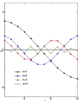
Figure 3: Eigenmodes for Massless quarks

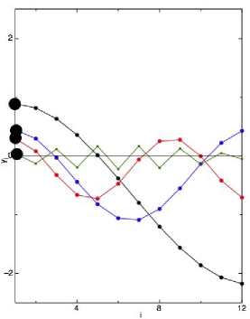
Figure 4: Eigenmodes for one massive, one massless quark

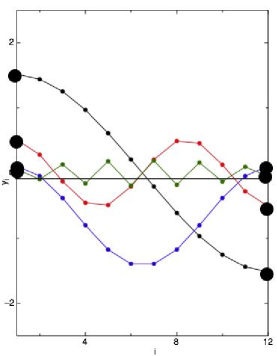
Figure 5: Eigenmodes for two massive quarks

Note that the heavy quarks stay relatively fixed, while the massless quarks move as much as the beads, as one would expect. The corresponding non-relativistic calculation shows simply a straight line for the ground state solution for the case with two massive quarks: in the relativistic case the beads necessarily carry a considerable amount of the energy.

The renomalised energies of the bound state are given by

$$\tilde{E}=\sum\limits_{i}{\tilde{\varepsilon}^{N}_{i}\left({n_{i},l_{i}}\right)}$$

where ${\tilde{\varepsilon}^{N}_{i}\left({n_{i},l_{i}}\right)}$ is given by (10) in the massless case. The only excited states we consider are the $l_{1}=1,l_{i>1}=0$ state, which corresponds to a conventional orbitally excited meson, and the $l_{1}=0,l_{2}=1,l_{i>2}=0$, which corresponds to the first hybrid state. If the quarks are massless, the ground state lies at $\tilde{E}^{0}=\sqrt{6\hbar c\sigma}\simeq 1GeV$ ( this would be lowered in a realistic model by the short-range colour interactions). Fig (6) shows the energies of the $l_{1}=1,l_{i>1}=0$ bound state as a function of quark mass for equal mass quarks and a varying number of beads. Note that the mass is dominated by the quark mass.

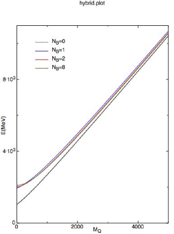
Figure 6: Total energies for states consisting of two massive quarks and a varying number of beads. The lowest curve is the ground state (identical for all $N_{B}$ by the renormalization process) and the upper curves show the energy for the $l_{1}=1$

It is more sensible to plot the excitation energy (i.e. the total energy with the quark mass subtracted), and in Fig (7) we show the ground state energy and the excitation energy of the 2 states for equal-mass quarks and varying number of beads.

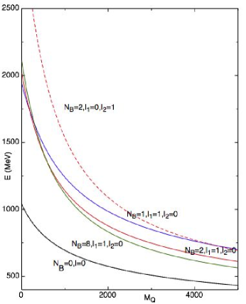
Figure 7: Excitation energies for states consisting of 2 massive quarks and a varying number of beads

Fig (8) is the corresponding plot for one heavy quark and one massless quark.

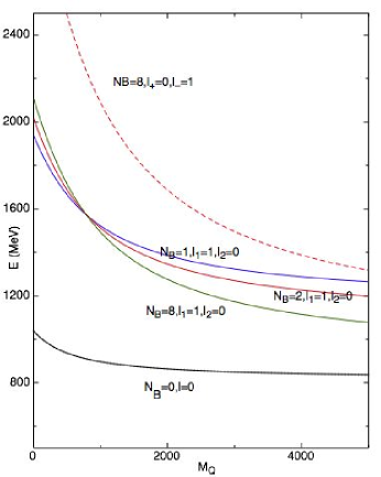
Figure 8: Excitation energies for states consisting of one massive and one massless quark and a varying number of beads

The energies are roughly independent of the number of beads. The energies typically lie lower as the number of beads increases. The hybrid state lies consistently at twice the excitation energy of the first orbitally excited state

VIII Conclusions

We have derived a relativistic model for mesons in a bead approximation to a flux-tube model. The model is analytically soluble for massless quarks, and can be renormalized to give a sensible spectrum. The massive quark case can be solved approximately by a rapidly converging algorithm. There are, however, several unattractive features.

1. The algorithm based on (19) implies that the amount of energy carried by the quarks decreases as the number of beads increases. This is artificial, but it is not clear whether it has any real physical consequence.

2. It is somewhat difficult to include short-range corrections: the colour Coulomb can be incorporated by a comparatively minor variation, as indicated, but the (crucial) hyperfine interactions probably require the extension of (5) to include a Dirac equation for the quarks.

3. It is difficult to consider radial excitations in the massive quark case.

4. The choice of the renormalized ground state energy is somewhat arbitrary.

These (and other) problems will be addressed in a later paper.

Appendix A Notation

There are several different energies in the calculation. They can be enumerated as follows:

1. $\varepsilon_{i}$ is the energy of the $i^{th}$ object (quark or bead)

2. $\hat{\varepsilon}_{i}^{N}\left({n_{i},l_{i}}\right)$ is the non-renormalized energy of the $i^{th}$ phonon mode, excited to an $\left({n_{i},l_{i}}\right)$ state, in the N-particle approximation.

3. $\tilde{\varepsilon}_{i}^{N}\left({n_{i},l_{i}}\right)$ is the renormalized energy of the $i^{th}$ phonon mode in the N-particle approximation.

4. $E^{N}\left({n_{i},l_{i}}\right)=\sum\limits_{i=1}^{N}{\hat{\varepsilon}_{i}^{N}\left({n_{i},l_{i}}\right)}$ is the non-renormalized energy of the bound state.

5. $E^{0}=E^{N}\left({0,0}\right)$ is the ground state energy for the meson.

6. $\tilde{E}^{N}\left({n_{k},l_{k}}\right)=\sum\limits_{i=1}^{N}{\tilde{\varepsilon}_{i}^{N}\left({n_{i},l_{i}}\right)}$ is the renormalized excited-state energy: i.e. the mass of the meson.

Appendix B Generic Variational Solution

In all the calculations, the variational value of the energy takes the following form:

$$\begin{array}[]{l}E^{2}=\sum\limits_{j}{d_{-2}^{j}\left({\alpha_{i}}\right)\beta_{j}^{2}}+\kappa Ed_{-1}\left({\beta_{k}}\right)+\\ d_{0}\left({\mu_{j},\alpha_{i}}\right)+\sigma d_{1}\left({\beta_{k},\mu_{j},\alpha_{i}}\right)+\frac{{\sigma^{2}}}{4}\sum\limits{\frac{{d_{2}^{k}\left({\alpha_{i}}\right)}}{{\beta_{k}^{2}}}}\\ \end{array}$$ (20)

with the following interpretations:

1. ${\beta_{k}}$ are the wave-function parameters.: i.e. $\psi\left({u_{i}}\right)=u_{i}^{l_{i}}e^{-\left({\beta_{i}u_{i}}\right)^{2}}$

2. The ${\alpha_{i}}$ are the energy separation parameters: see (19

3. ${d_{-2}^{k}\left({\alpha_{i}}\right)}$ is the KE term: e.g for the 2-bead case with no Coulomb interaction,

   $$\begin{array}[]{l}d_{-2}^{+}\left({\alpha_{i}}\right)=\frac{{\hbar^{2}c^{2}}}{{\alpha_{1}\alpha_{B}}}\left({\frac{3}{2}+l_{+}}\right)\\ d_{-2}^{-}\left({\alpha_{i}}\right)=\frac{{\hbar^{2}c^{2}}}{{\alpha_{B}}}\left({\frac{3}{2}+l_{-}}\right)\\ \end{array}$$

4. ${d_{-1}\left({\beta_{k}}\right)}$ is Coulomb correction: note that it contains E since it is the 4th component of a 4-vector.

5. ${d_{0}\left({\mu_{j},\alpha_{i}}\right)}$ is the mass term:

   $$d_{0}\left({\mu_{j},\alpha_{i}}\right)=\frac{{\mu_{1}^{2}}}{{\alpha_{1}}}+\frac{{\mu_{2}^{2}}}{{\alpha_{2}}}$$

   so vanishes for massless quarks,

6. ${d_{1}\left({\alpha_{i},\mu_{j},\beta_{k}}\right)}$ is the linear potential term:

   $$d_{1}\left({\alpha_{i},\mu_{j},\beta_{k}}\right)=\left({\frac{{\mu_{1}}}{{\alpha_{1}}}+\frac{{\mu_{2}}}{{\alpha_{2}}}}\right)\frac{2}{{\beta\sqrt{\pi}}}$$

   for 0-bead and

   $$\begin{array}[]{l}d_{1}\left({\alpha_{i},\mu_{j},\beta_{i}}\right)=\left({\frac{{\mu_{1}}}{{\alpha_{1}}}f^{\left(1\right)}+\frac{{\mu_{N}}}{{\alpha_{N}}}f^{\left(N\right)}}\right),\\ f^{\left(m\right)}\approx\sqrt{\frac{3}{2}}\left({\sum\limits_{i}^{N}{\frac{{e_{im}^{2}}}{{\beta_{i}^{2}}}}}\right)^{1/2}\\ \end{array}$$

   for the $N_{B}$-bead case.

7. ${d_{2}^{k}\left({\alpha_{i}}\right)}$ arises from square of the linear terms:

   $$d_{2}^{+}\left({\alpha_{i}}\right)=\left({\frac{3}{2}+l_{-}}\right),d_{2}^{-}\left({\alpha_{i}}\right)=\frac{{\left({\frac{3}{2}+l_{+}}\right)}}{{\alpha_{B}}}$$

   for 1-bead case

The merit of writing it in this form is that it is completely general and has an immediate solution for massless quarks with no Coulomb interaction:

$$d_{-2}^{i}\left({\alpha_{i}}\right)=\Lambda_{i}^{N},d_{2}^{i}\left({\alpha_{i}}\right)=\Lambda_{N-i}^{N},d_{-1}^{i}=d_{0}^{i}=d_{1}^{i}=0$$

gives

$$\left({\beta_{i}^{N}}\right)^{2}=\sqrt{\frac{{\Lambda_{N-i}}}{{\Lambda_{i}}}}\frac{\sigma}{2}$$

The general solution for the non-linear equation set can be written

$$\begin{array}[]{l}\beta_{k}=\left[{\frac{{\frac{{2\sigma^{2}}}{4}d_{2}^{k}\left({\alpha_{i}}\right)-\kappa E\left({\alpha_{i},\beta_{k}}\right)\beta_{k}^{3}\frac{{\partial d_{-1}\left({\beta_{i}}\right)}}{{\partial\beta_{k}}}+\sigma\beta_{k}^{3}\frac{{\partial d_{1}\left({\beta_{i}}\right)}}{{\partial\beta_{k}}}}}{{2d_{-2}^{k}\left({\alpha_{i}}\right)}}}\right]^{1/4}\\ =H_{k}\left({\beta_{i},\beta_{k}}\right)\\ \end{array}$$ (21)

This is the basis of the algorithm for rapid solution of the general case:

1. Start with the above

   $$\beta_{i0}=\left({\frac{{d_{2}^{i}\left({\alpha_{i}}\right)}}{{d_{-2}^{i}\left({\alpha_{i}}\right)}}}\right)^{1/4}$$

2. Fix all ${\beta_{i}}$ except for one, ${\beta_{k}}$.

3. Find 3 successive values of ${\beta_{k}}$ using eqn. (21)

   $$\beta_{k}^{\left(n\right)}=H\left({\beta_{i},\beta_{k}^{\left({n-1}\right)}}\right)$$

4. FInd the Aiken extrapolation to provide an updated ${\beta_{k}}$

   $$\beta_{k}=\frac{{\beta_{k}^{\left(2\right)}\beta_{k}^{\left(0\right)}-\left({\beta_{k}^{\left(1\right)}}\right)^{2}}}{{\beta_{k}^{\left(2\right)}-2\beta_{k}^{\left(1\right)}+\beta_{k}^{\left(0\right)}}}$$

5. Choose another ${\beta_{k^{\prime}}}$ and iterate until the values converge (typically 3 iterations for the full set).

6. Use the final values of the ${\beta_{i}}$ to find the energy E using 20.

Ths works very rapidly because

$$\frac{{\beta_{k}^{3}\partial d_{1}\left({\alpha_{i},\mu_{j},\beta_{i}}\right)}}{{\partial\beta_{k}}}=-\frac{3}{2}\left({\frac{{\mu_{1}}}{{\alpha_{1}}}\frac{{e_{i1}^{2}}}{{f^{\left(1\right)}}}+\frac{{\mu_{N}}}{{\alpha_{N}}}\frac{{e_{iN}^{2}}}{{f^{\left(N\right)}}}}\right)$$

is a comparatively slowly varying function of the ${\beta_{i}}$.

There is an extra complication when the Coulomb term is included because the energy needs to be calculated after each of the ${\beta_{i}}$ are estimated. Note that this format of the equation retains the phonon picture.

Appendix C Standard Integrals

For the one-bead case, we need to define a standard integral

$$\begin{array}[]{l}g_{l_{+}l_{-}}^{k}\left({\beta_{+},\beta_{-}}\right)=\\ \int{\int{u_{+}^{2l_{+}}e^{-\beta_{+}^{2}u_{+}^{2}}u_{-}^{2l_{-}}e^{-\beta_{-}^{2}u_{-}^{2}}\left|{\hat{u}_{+}^{2}+\hat{u}_{-}^{2}}\right|^{k/2}u_{+}^{2}u_{-}^{2}du_{+}du_{-}}}\\ =\int{\int\begin{array}[]{l}e^{-y^{2}\left({\beta_{+}^{2}\cos^{2}\left(\phi\right)+\beta_{-}^{2}\sin^{2}\left(\phi\right)}\right)}\\ \cos^{2+2l_{+}}\left(\phi\right)\sin^{2+2l_{-}}\left(\phi\right)y^{5+2l_{+}+2l_{-}+k}dyd\phi\\ \end{array}}\\ =\frac{{\Gamma\left({3+l_{+}+l_{-}+\frac{k}{2}}\right)}}{2}\\ \int{\frac{{\cos^{{}^{2+2l_{+}}}\left(\phi\right)\sin^{{}^{2+2l_{-}}}\left(\phi\right)}}{{\left({\beta_{+}^{2}\cos^{2}\left(\phi\right)+\beta_{-}^{2}\sin^{2}\left(\phi\right)}\right)^{3+l_{+}+l_{-}+\frac{k}{2}}}}d\phi}\\ \end{array}$$

since the y integral is trivial. Then the k = 0 term is just the normalization:

$$\frac{1}{{A^{2}}}=g_{l_{+}l_{-}}^{0}\left({\beta_{+},\beta_{-}}\right)=\frac{{\Gamma\left({\frac{3}{2}+l_{+}}\right)\Gamma\left({\frac{3}{2}+l_{-}}\right)}}{{4\beta_{+}^{3+2l_{+}}\beta_{-}^{3+2l_{-}}}}$$

so that

$$\begin{array}[]{l}f_{l_{+}l_{-}}^{k}\left({\beta_{+},\beta_{-}}\right)=\frac{{g_{l_{+}l_{-}}^{k}\left({\beta_{+},\beta_{-}}\right)}}{{A^{2}}}\\ =\frac{{2\Gamma\left({3+l_{+}+l_{-}+\frac{k}{2}}\right)\beta_{+}^{3+2l_{+}}\beta_{-}^{3+2l_{-}}}}{{\Gamma\left({\frac{3}{2}+l_{+}}\right)\Gamma\left({\frac{3}{2}+l_{-}}\right)}}\times\\ \int{\frac{{\cos^{{}^{2+2l_{+}}}\left(\phi\right)\sin^{{}^{2+2l_{-}}}\left(\phi\right)}}{{\left({\beta_{+}^{2}\cos^{2}\left(\phi\right)+\beta_{-}^{2}\sin^{2}\left(\phi\right)}\right)^{3+l_{+}+l_{-}+\frac{k}{2}}}}d\phi}\\ \end{array}$$

This cannot be evaluated analytically for for k odd. However, checks that can be run include:

$$f_{l_{+}l_{-}}^{0}\left({\beta_{+},\beta_{-}}\right)=1,f_{l_{+}l_{-}}^{2}\left({\beta_{+},\beta_{-}}\right)=\frac{{\left({l_{+}+\frac{3}{2}}\right)}}{{\beta_{+}^{2}}}+\frac{{\left({l_{-}+\frac{3}{2}}\right)}}{{\beta_{-}^{2}}}$$

so approximately

$$f_{l_{+}l_{-}}^{1}\left({\beta_{+},\beta_{-}}\right)=\left({\frac{{\left({l_{+}+\frac{3}{2}}\right)}}{{\beta_{+}^{2}}}+\frac{{\left({l_{-}+\frac{3}{2}}\right)}}{{\beta_{-}^{2}}}}\right)^{1/2}$$

Appendix D n-body Interactions

The trick in the previous section does not work for an $N_{B}$-bead solution with massive quarks, Instead we need to evaluate the expectation values of terms like

$$\left|{\hat{r}_{1}}\right|=\sqrt{\hat{r}_{1}^{2}}=\sqrt{\left({\sum\limits{e_{j}^{\left(1\right)}u_{j}}}\right)^{2}}=\sqrt{\sum\limits{e_{j}^{\left(1\right)}e_{k}^{\left(1\right)}u_{j}u_{k}}}$$

We cannot evaluate $\int{\left|{\hat{r}_{1}}\right|^{k}}e^{-\sum\limits{\beta_{i}^{2}u_{i}^{2}}}\Pi u_{i}^{2}du_{i}$ for k = 1 directly. Write

$$\begin{array}[]{l}F^{N}\left({\beta_{i}}\right)=C\int{\left|{\sum\limits{e_{i}^{2}u_{i}^{2}}}\right|^{1/2}\prod\limits_{i}^{N}{e^{-\beta_{i}^{2}u_{i}^{2}}}}u_{i}^{2}du_{i}\\ E_{n}=\sum\limits_{i=n+1}^{N}{e_{i}^{2}u_{i}^{2}},B_{n}=\frac{3}{2}\sum\limits_{i=1}^{n}{\frac{{e_{i}^{2}}}{{\beta_{i}^{2}}}}\\ \end{array}$$

(C is the normalisation). Then we can expand, integrate and contract:

$$\begin{array}[]{l}\int{\left|{\sum\limits{e_{i}^{2}u_{i}^{2}}}\right|^{1/2}e^{-\beta_{1}^{2}u_{1}^{2}}u_{1}^{2}du_{1}}=\int{\left|{A_{1}+e_{1}^{2}u_{1}^{2}}\right|^{1/2}e^{-\beta_{1}^{2}u_{1}^{2}}u_{1}^{2}du_{1}}\\ \approx\left({A_{1}+B_{1}}\right)^{1/2}=\left({A_{2}+B_{1}+e_{2}^{2}u_{2}^{2}}\right)^{1/2}\\ \end{array}$$

or in general

$$\int{\left|{A_{n}+B_{n-1}+e_{n}^{2}u_{n}^{2}}\right|^{1/2}e^{-\beta_{n}^{2}u_{n}^{2}}u_{n}^{2}du_{n}}\approx\left({A_{n}+B_{n}}\right)^{1/2}$$

Repeating this gives

$$F^{N}\left({\beta_{i}}\right)\approx\sqrt{B_{N}}=\left({\frac{3}{2}\sum\limits_{i=n-1}^{N}{\frac{{e_{i}^{2}}}{{\beta_{i}^{2}}}}}\right)^{1/2}$$

. All the cross terms vanish on integration.

We can extend this: e.g. Coulomb term only exists between quarks, so write

$$\begin{array}[]{l}\frac{1}{{\left|{\vec{r}_{1}-\vec{r}_{N}}\right|}}=\frac{1}{{\left|{\vec{r}_{1}-\vec{r}_{2}+\vec{r}_{2}-\vec{r}_{3}+...-\vec{r}_{N}}\right|}}\\ =\frac{1}{{\left|{\sum\limits{\hat{r}_{i}}}\right|}}=\left({\sum\limits_{jl}{\hat{u}_{j}\hat{u}_{l}}\sum\limits_{ik}{e_{k}^{l}e_{i}^{j}}}\right)^{-1/2}\\ \end{array}$$

giving the expectation value

$$F_{m}^{C}\left({\beta_{i}}\right)\approx\left({\frac{3}{2}\sum\limits_{i=n-1}^{N}{\frac{{b_{i}^{C}}}{{\beta_{i}^{2}}}}}\right)^{1/2},b_{i}^{C}=\sum\limits_{jk}{e_{j}^{i}e_{k}^{i}}$$

References

- Isgur and Paton (1985) N. Isgur and J. E. Paton, Phys. Rev. D31, 2910 (1985).
- Bali (2000) G. S. Bali (2000), eprint hep-ph/0010032.
- Morningstar (2003) C. Morningstar, in Workshop on Gluonic Excitations (2003).
- Allen et al. (1998) T. J. Allen, M. G. Olsson, and S. Veseli, Phys. Lett. B434, 110 (1998), eprint hep-ph/9804452.
- Merlin and Paton (1985) J. Merlin and J. Paton, J. Phys. G11, 439 (1985).
- Swanson (2003) E. S. Swanson (2003), eprint hep-ph/0311328.
- Close and Dudek (2004) F. E. Close and J. J. Dudek, Phys. Rev. D69, 034010 (2004), eprint hep-ph/0308098.
- Barnes et al. (1995) T. Barnes, F. E. Close, and E. S. Swanson, Phys. Rev. D52, 5242 (1995), eprint hep-ph/9501405.
- Ram (1982) B. Ram, American Journal of Physics 50, 549 (1982), URL http://link.aip.org/link/?AJP/50/549/1.
- Ebert et al. (1998) D. Ebert, V. O. Galkin, and R. N. Faustov, Phys. Rev. D57, 5663 (1998), eprint hep-ph/9712318.
- Yueh (2005) W.-C. Yueh, App. Math E-notes 5, 66 (2005).
- Olsson (1997) M. G. Olsson, Phys. Rev. D56, 238 (1997), eprint hep-ph/9702213.