Decay Constants of Pseudo-scalar Mesons in Bethe-Salpeter Framework with Generalized Structure of Hadron-Quark Vertex

Abstract

We employ the framework of Bethe-Salpeter equation under Covariant Instantaneous Ansatz to study the leptonic decays of pseudo-scalar mesons. The Dirac structure of hadron-quark vertex function $\Gamma$ is generalized to include various Dirac covariants besides $\gamma_{5}$ from their complete set. The covariants are incorporated in accordance with a power counting rule, order by order in powers of the inverse of the meson mass. The decay constants are calculated with the incorporation of leading order covariants. Most of the results are dramatically improved.

PACS: 11.10.St, 12.39.Ki, 13.20.-v, 13.20.Jf

1 Introduction

Quantum Chromodynamics (QCD) is regarded as the correct theory for strong interactions. Investigation of bound states of quarks (and/or gluons) is one of the most effective methods to study this dynamics among these constituents. Since the task of calculating hadron structure from QCD itself is very difficult (as can be seen from various lattice QCD methods), one can on the other hand rely on specific models to gain some understanding of it at low energies, and this study can most effectively be accomplished by applying a particular framework to a diverse range of phenomena. Meson decays provide an important opportunity for exploring the structure of these simplest bound states in QCD and for studying the non-perturbative (long distance) aspect of the strong interactions. Besides vector mesons (see, e.g., [1] and refs. therein), pseudo-scalar mesons have for a long time been a major focus of attention to understand the inner structure of hadrons from non-perturbative QCD. A number of such studies [2, 3, 4, 5, 6, 7] dealing with decays of pseudo-scalar mesons at quark level of compositeness have been carried out recently. In this paper, we study leptonic decays of pseudo-scalar mesons such as $K$, $D$, $D_{S}$ and $B$, which proceed through the coupling of the quark-antiquark loop to the axial vector current as shown in Figure 1.

A realistic description of pseudo-scalar mesons at the quark level of compositeness would be an important element in our understanding of hadron dynamics and reaction processes at scales where QCD degrees of freedom are relevant. Such studies offer a direct probe of hadron structure and help in revealing some aspects of the underlying quark-gluon dynamics. The relativistic description for analyzing mesons as composite objects is provided by the framework of Bethe-Salpeter Equation (BSE) in this paper. We employ the QCD oriented BSE under Covariant Instantaneous Ansatz (CIA) [8]. CIA is a Lorentz-covariant generalization of Instantaneous Approximation. For $q\bar{q}$ system, CIA formulation [8] ensures an exact interconnection between 3D and 4D forms of the BSE. The 3D form of BSE serves for making contact with the mass spectra, whereas the 4D form provides the $Hq\bar{q}$ vertex function $\Gamma(\widehat{q})$ for the evaluation of various transition amplitudes. A BSE framework under Instantaneous Approximation formulation similar to the CIA formulation was also earlier suggested by the Bonn group [9].

We had earlier employed the framework of BSE under CIA for calculation of decay constants [8, 10] of heavy-light pseudo-scalar mesons and $F_{\pi}$ for $\pi^{0}\rightarrow 2\gamma$ process. We also evaluated the leptonic decays of vector mesons, such as $\rho$, $\omega$, $\phi$ [11] in this framework. However, one of the simplified assumptions in all these calculations was that the $Hq\bar{q}$ vertex was restricted to have a single Dirac structure (e.g., $\gamma_{5}$ for pseudo-scalar mesons, $\gamma\cdot\varepsilon$ for vector mesons, etc.). However, recent studies [5, 12, 13] have revealed that various mesons have many different covariant structures in their wave functions whose inclusion was also found necessary to obtain quantitatively accurate observables [12] and it was further noticed that all Dirac covariants do not contribute equally and only some of them are relevant for calculation of meson mass spectrum and decay constants. Such a copious Dirac structure of the BS wave function in fact was already indicated by Llewellyn Smith [14]. Hence it is necessary to introduce various Dirac structures into the $Hq\bar{q}$ vertex for different kinds of mesons. In the recent work [1], we developed a power counting rule for incorporating various Dirac covariants in the structure of vertex function, order by order in powers of inverse of meson mass, and calculated the leptonic decays of equal mass vector mesons such as $\rho$, $\omega$, $\phi$, taking into account the leading order covariants since they are expected to contribute maximum to observables according to our scheme. On the line of that work, in this paper we first discuss the power counting rule for choosing various Dirac covariants from their complete set (see, e.g., [5, 12, 13, 14]) for pseudo-scalar mesons in Section 2. In section 3 we calculate leptonic decay constants of them employing the wave function developed in section 2. We then conclude with discussions in Section 4.

2 Structure of generalized vertex function $\Gamma(\widehat{q})$ for pseudo-scalar mesons in BSE under CIA

For introducing the variables and for the convenience to discuss the generalized hadron-quark vertex in BS wave function under CIA, we give the similar outline for CIA as in Ref. [1, 11]. We start with a 4D BSE for scalar $q\bar{q}$ system with an effective kernel $K$ and 4D wave function $\Phi(P,q)$:

$$i(2\pi)^{4}\Delta_{1}\Delta_{2}\Phi(P,q)=\int{d^{4}}q^{\prime}K(q,q^{\prime})\Phi(P,q^{\prime}),$$ (1)

where $\Delta_{1,2}$, the inverse propagators of two scalar quarks, are:

$$\Delta_{1,2}=m_{1,2}^{2}+p_{1,2}^{2}.$$ (2)

Here $m_{1,2}$ are (effective) constituent masses of quarks. The 4-momenta of the quark and anti-quark, $p_{1,2}$, are related to the internal 4-momentum $q_{\mu}$ and total momentum $P$ of hadron of mass $M$ as

$$p_{1,2}{}_{\mu}=\hat{m}_{1,2}P_{\mu}\pm q_{\mu},$$ (3)

where $\hat{m}_{1,2}=[1\pm(m_{1}^{2}-m_{2}^{2})/M^{2}]/2$ are the Wightman-Garding (WG) definitions [10] of masses of individual quarks.

The CIA Ansatz on the BS kernel $K$ in Eq. (1) is,

$$K(q,q^{\prime})=K(\hat{q},\hat{q}^{\prime}),$$ (4)

where

$$\hat{q}_{\mu}=q_{\mu}-\frac{q\cdot P}{P^{2}}P_{\mu}$$ (5)

is observed to be orthogonal to the total 4-momentum $P$ ( i.e., $\hat{q}.P=0)$, irrespective of whether the individual quarks are on-shell or off-shell. A similar form of the BS kernel was also suggested in ref. [9]. The longitudinal component of $q_{\mu}$,

$$M\sigma=M\frac{q\cdot P}{P^{2}},$$ (6)

does not appear in the form $K(\hat{q},\hat{q}^{\prime})$ of the kernel. For reducing Eq. (1) to the 3D form, one can define a 3D wave function $\phi(\widehat{q})$ as

$$\phi(\widehat{q})=\int\limits_{-\infty}^{+\infty}{Md\sigma\Phi(P,q)}.$$ (7)

Following usual steps outlined in [1, 8, 11], we get the $Hq\bar{q}$ vertex function $\Gamma(\hat{q})$ under CIA for the case of scalar quarks:

$$\Delta_{1}\Delta_{2}\Phi(P,q)=\frac{D(\widehat{q})\phi(\widehat{q})}{2\pi i}\equiv\Gamma(\widehat{q})\quad~{}\quad\frac{1}{D(\widehat{q})}=\frac{1}{2\pi i}\int\limits_{-\infty}^{+\infty}{\frac{Md\sigma}{\Delta_{1}\Delta_{2}}},$$ (8)

where $D(\widehat{q})$ is a 3D denominator function whose value can be easily worked out by contour integration by noting the positions of the poles in the complex $\sigma-$plane [1, 8, 11]. By this process, an exact interconnection between 3D wave function $\phi(\widehat{q})$ and the 4D wave function $\Phi(P,q)$ and hence that between 3D and 4D BSE is thus brought out, where the 3D form serves for making contact with the mass spectrum of hadrons, whereas the 4D form provides the $Hq\bar{q}$ vertex function $\Gamma(\hat{q})$ which satisfies a 4D BSE with a natural off-shell extension over the entire 4D space (due to the positive definiteness of the quantity $\hat{q}^{2}=q^{2}-\frac{(q\cdot P)^{2}}{P^{2}}$ throughout the entire 4D space) and thus provides a fully Lorentz-covariant basis for evaluation of various transition amplitudes through various quark loop diagrams (see Figure 1).

To apply the above simplified discussions to the case of fermionic quarks constituting a particular meson we proceed in the same manner as [1]: The scalar propagators $\Delta_{i}^{-1}$ in the above equations are replaced by the proper fermionic propagators $S_{F}$. Then, on observing the vertex $\Gamma(\hat{q})$ now is a $4\times 4$ matrix in the spinor space, we should incorporate its relevant Dirac structures, for which we take guidance from some recent studies [5, 12, 13], as well as Llewelyn-Smith’s classic paper [14], which have revealed that various mesons have many different covariant structures in their wave functions whose inclusion was found necessary to obtain quantitatively accurate observables. It was also noticed recently [12] that all Dirac covariants do not contribute equally and only some covariants are considered to be relevant for calculation of mass spectrum and decay constants. Ref. [12] has also calculated masses and decay constants of vector mesons for various subsets of covariants from their complete set. Towards this end, we make use of the power counting rule developed in [1] for incorporating various Dirac covariants in the structure of $Hq\bar{q}$ vertex function for a particular meson, order-by-order in powers of inverse of the meson mass $M$, so as to systematically choose among various covariants from their complete set and write wave functions for various mesons.

As far as a pseudo-scalar meson is concerned, its $Hq\bar{q}$ vertex function, which has a certain dimensionality of mass, can be expressed as a linear combination of four Dirac covariants $\Gamma_{i}^{P}(i=0,...,3)$ [12, 13, 14], each multiplying a Lorentz scalar amplitude $F_{i}(q^{2},q\cdot P,P^{2})$. The choice of the Dirac covariants is not unique as can also be seen from the choice of covariants used in Ref. [12, 13]. For adapting this decomposition to write the structure of vertex function $\Gamma(\hat{q})$, we re-express the $Hq\bar{q}$ vertex function by making the amplitudes $F_{i}(q^{2},q\cdot P,P^{2})$ dimensionless, weighing each Dirac covariant with an appropriate power of $M$. Thus each term in the expansion of $\Gamma(\hat{q})$ is associated with a certain power of $M$. In detail, we can express $\Gamma_{P}$ as a polynomial in various powers of $1/M$:

$$\Gamma_{P}=\Omega_{P}\frac{1}{2\pi i}N_{P}D(\hat{q})\phi(\hat{q}),$$ (9)

with

$$\Omega_{P}=\gamma_{5}B_{0}-i\gamma_{5}(\gamma\cdot P)\frac{B_{1}}{M}-i\gamma_{5}(\gamma\cdot q)\frac{B_{2}}{M}-\gamma_{5}(\gamma\cdot P\gamma\cdot q-\gamma\cdot q\gamma\cdot P)\frac{B_{3}}{M^{2}}.$$ (10)

Here $B_{i}(i=0,...,3)$ are four dimensionless and constant coefficients (which are taken to be constant on lines of [1], only to consider the leading powers of $1/M$) to be determined. Now since we use constituent quark masses where the quark mass $m$ is approximately half of the hadron mass $M$, we can use the ansatz

$$q<<P\sim M$$ (11)

in the rest frame of the hadron (among all the pseudo-scalar mesons, pion enjoys the special status in view of its unusually small mass ($<\Lambda_{QCD}$) and its case should be considered separately. See the discussions in Section 4). Then each of the four terms in Eq. (9) receives suppression by different powers of $1/M$. Thus we can arrange these terms as an expansion in powers of $O(\frac{1}{M})$. We can see in the expansion of $\Omega_{P}$ that the structures associated with the coefficients $B_{0},B_{1}$ have magnitudes $O(\frac{1}{M^{0}})$ and are of leading order, while those with $B_{2},B_{3}$ are $O(\frac{1}{M^{1}})$and are next-to-leading order. This naïve power counting rule suggests that the maximum contribution to the calculation of any pseudo-scalar meson observable should come from the leading order Dirac structures $\gamma_{5}$ and $i\gamma_{5}(\gamma.P)\frac{1}{M}$ associated with the constant coefficients $B_{0}$ and $B_{1}$, respectively. As a first application of this to the pseudo-scalar meson sector and on lines similar to [1] for vector meson case, we take the form of the $Hq\bar{q}$ vertex function incorporating the leading order terms in expansion (9) and ignoring $O(\frac{1}{M^{1}})$ terms for the moment, i.e.,

$$\Gamma(\hat{q})=[\gamma_{5}B_{0}-i\gamma_{5}\gamma\cdot P\frac{B_{1}}{M}]\frac{1}{2\pi i}N_{P}D(\hat{q})\phi(\hat{q})\quad.$$ (12)

As has been stated in [1], the restriction from charge Parity on the wave function of the eigenstate should be respected .

From the above analysis of the structure of $Hq\bar{q}$ vertex function in Eq.(12) we notice that, at leading order, the structure of 3D wave function $\phi(\hat{q})$ as well as the form of the 3D BSE are left untouched and have the same form as in our previous works, which justifies the usage of the same form of the input kernel we used earlier. Now we briefly mention some features of the BS formulation employed. The structure of BSE is characterized by a single effective kernel arising out of a four-fermion Lagrangian in the Nambu-Jonalasino [15, 16] sense. The formalism is fully consistent with Nambu-Jona-Lasino [16] picture of chiral symmetry breaking but is additionally Lorentz-invariant because of the unique properties of the quantity $\hat{q}^{2}$, which is positive definite throughout the entire 4D space. The input kernel $K(q,q^{\prime})$ in BSE is taken as one-gluon-exchange like as regards color ($\frac{1}{2}\vec{\lambda}.\frac{1}{2}\vec{\lambda}_{2})$ and spin ($\gamma_{\mu}^{(1)}\gamma_{\mu}^{(2)})$ dependence. The scalar function $V(q-q^{\prime})$ is a sum of one-gluon exchange $V_{OGE}$ and a confining term $V_{Conf.}$ [1, 11, 15]. Thus

$$K(q,q^{\prime})=\frac{1}{2}\vec{\lambda}^{(1)}\frac{1}{2}\vec{\lambda}^{(2)}V_{\mu}^{(1)}V_{\mu}^{(2)}V(q-q^{\prime});$$

$$V_{\mu}^{(1,2)}=\pm 2m_{1,2}\gamma_{\mu}^{(1,2)};$$

$$V(\hat{q}-\hat{q}^{\prime})=\frac{4\pi\alpha_{S}(Q^{2})}{(\hat{q}-\hat{q}^{\prime})^{2}}+\frac{3}{4}\omega_{q\bar{q}}^{2}\int{d^{3}\vec{r}[r^{2}}(1+4a_{0}\hat{m}_{1}\hat{m}_{2}M_{>}^{2}r^{2})^{-\frac{1}{2}}-\frac{C_{0}}{\omega_{0}^{2}}]e^{i(\hat{q}-\hat{q}^{\prime})\cdot\vec{r}};$$ (13)

$$\alpha_{S}(Q^{2})=\frac{12\pi}{33-2f}\left[{\ln\frac{M_{>}^{2}}{\Lambda^{2}}}\right]^{-1};~{}~{}M_{>}=Max(M,m_{1}+m_{2}).$$ (14)

The ansatz employed for the spring constant $\omega_{q\overline{q}}^{2}$ in the above equation is [1,11,15]

$$\omega_{q\overline{q}}^{2}=4\widehat{m}_{1}\widehat{m}_{2}M_{>}\omega_{0}^{2}\alpha_{S}(Q^{2}).$$ (15)

Here the proportionality of $\omega_{q\overline{q}}^{2}$ on $\alpha_{S}(Q^{2})$ is needed to provide a more direct QCD motivation to confinement. This assumption further facilitates a flavour variation in $\omega_{q\overline{q}}^{2}$. And $\omega_{0}^{2}$ in Eq.(13) and Eq.(14) is postulated as a universal spring constant which is common to all flavours.

In the expression for $V(\hat{q}-\hat{q}^{\prime})$, as far as the integrand of confining term $V_{Conf.}$ is concerned, the constant term $C_{0}/\omega_{0}^{2}$ is designed to take into account the correct zero point energies, while $a_{0}$ term ($a_{0}<<1)$ simulates an effect of an almost linear confinement for heavy quark sectors (large $m_{1},m_{2}$ ), retaining the harmonic form for light quark sectors (small $m_{1},m_{2})$ [1, 15], as is believed to be true for QCD. Hence the term ${r^{2}}(1+4a_{0}\hat{m}_{1}\hat{m}_{2}M_{>}^{2}r^{2})^{-\frac{1}{2}}$ in the above expression is responsible for effecting a smooth transition from harmonic ($q\overline{q}$) to linear ($Q\overline{Q}$) confinement. The values of basic input parameters of the model are $a_{0}=.028,~{}C_{0}=.29,~{}\omega_{0}=.158~{}(GeV)$ and $\Lambda=.20GeV$ [1,10,11,15] which have been calibrated to fit the $q\overline{q}$ hadron mass spectrum obtained by solving the 3D BSE [15].

Now comes to the problem of the 3D BS wave function. The ground state wave function $\phi(\widehat{q})$ satisfies the 3D BSE [1] on the surface P.q = 0, which is appropriate for making contact with O(3)-like mass spectrum [15]. Its fuller structure (described in Ref. [15]) is reducible to that of a 3D harmonic oscillator with coefficients dependent on the hadron mass M and the total quantum number N. The ground state wave function $\phi(\hat{q})$deducible from this equation thus has a Gaussian structure [1, 8, 11] and is expressible as:

$$\phi(\widehat{q})\approx e^{-\widehat{q}^{2}/2\beta^{2}}.$$ (16)

In the structure of $\phi(\hat{q})$ in Eq. (16), the parameter $\beta$ is the inverse range parameter which incorporates the content of BS dynamics and is dependent on the input kernel $K(q,q^{\prime})$. The structure of $\beta$ is given in Section 3.

3 Decays constants $f_{P}$ of Pseudo-scalar Mesons

Decay constants $f_{P}$ can be evaluated through the loop diagram shown in Figure 1 which gives the coupling of the two-quark loop to the axial vector current and can be evaluated as:

$$f_{P}P_{\mu}=<0|\bar{Q}i\gamma_{\mu}\gamma_{5}Q|P(P)>,$$ (17)

which can in turn be expressed as a loop integral:

$$f_{P}P_{\mu}=\sqrt{3}\int{d^{4}}qTr[\Psi_{P}(P,q)i\gamma_{\mu}\gamma_{5}]\quad.$$ (18)

Bethe-Salpeter wave function $\Psi(P,q)$ for a P-meson is expressed as

$$\Psi(P,q)=S_{F}(p_{1})\Gamma(\hat{q})S_{F}(-p_{2}), with~{}~{}~{}~{}$$

$$S_{F}(p_{1})=-i\frac{(m_{1}-i\gamma\cdot p_{1})}{\Delta_{1}}; S_{F}(-p_{2})=-i\frac{(m_{2}+i\gamma\cdot p_{2})}{\Delta_{2}}.$$ (19)

In the following calculation, we only take the leading order terms in the structure of hadron-quark vertex function $\Gamma(\hat{q})$ as in Eq. (12). $S_{F}$ are the fermionic propagators for the two constituent quarks of the hadron and the non-perturbative aspects enter through the $\Gamma(\widehat{q})$. Using $\Psi(P,q)$ from Eq.(19) and the structure of $Hq\bar{q}$ vertex $\Gamma(\hat{q})$ from Eq.(12), evaluating trace over $\gamma$-matrices and multiplying both sides of Eq.(18) by $P_{\mu}/(-M^{2})$, we can express $f_{P}$ as:

$$f_{P}=\sqrt{3}N_{P}\int{d^{3}}\hat{q}D(\hat{q})\phi(\hat{q})I\quad,$$

$$I = \int\limits_{-\infty}^{+\infty}{\frac{Md\sigma}{2\pi i\Delta_{1}\Delta_{2}}}\{2B_{0}[m_{12}(1-\frac{\delta m^{2}}{M^{2}})+2\delta m\sigma]$$

$$+ \frac{B_{1}}{M^{3}}[(-M^{4}-4m_{1}m_{2}M^{2}+m_{12}^{2}\delta m^{2})+4M^{2}\hat{q}^{2}-4M^{2}m_{12}\delta m\sigma+4M^{4}\sigma^{2}]\},$$

where according to Eq.(3) and Eq.(5), we had expressed scalar products $p_{1}\cdot p_{2}$, $p_{1}\cdot P$and $p_{2}\cdot P$ as

$$p_{1}.p_{2}=-M^{2}(\hat{m}_{1}+\sigma)(\hat{m}_{2}-\sigma)-\hat{q}^{2},$$ (21)

$$\begin{array}[]{l}p_{1}\cdot P=-M^{2}(\hat{m}_{1}+\sigma)\\ p_{2}\cdot P=-M^{2}(\hat{m}_{2}-\sigma),\end{array}$$

with $m_{12}=m_{1}+m_{2}$ and $\delta m=m_{2}-m_{1}$. Here we have employed unequal mass kinematics when the hadron constituents have different masses. We see that on the right hand side of the expression for $f_{P}$, each of the expressions multiplying the constant parameters $B_{0}$ and $B_{1}$ consist of two parts, of which only the second part explicitly involves the off-shell parameter $\sigma$ (that is terms involving $\sigma$ multiplying $B_{0}$, and terms involving both $\sigma$ and $\sigma^{2}$ multiplying $B_{1})$). It is seen that the off-shell contribution which vanishes for $m_{1}=m_{2}$ in case of $f_{P}$ calculation in CIA [10] using only the covariant $\gamma_{5}$, now no longer vanishes for $m_{1}=m_{2}$ in the above calculation, due to the term $4M^{4}\sigma^{2}$ multiplying $B_{1}$ when another leading order covariant $i\gamma_{5}\gamma\cdot P/M$ is also incorporated in $Hq\bar{q}$ vertex function. This possibly implies that the off-shell part of $f_{P}$ does not arise from unequal mass kinematics alone, which is in complete contrast to the earlier CIA calculation of $f_{P}$ [10] employing only $\gamma_{5}$. This serves as a clear pointer to the fact that in this BS-CIA model, the Dirac covariants other than $\gamma_{5}$ might also be important for the study of processes involving large $q^{2}$ (off-shell), which is also suggested in [17].

Carrying out integration over $d\sigma$ by noting the pole positions in the complex $\sigma$-plane

$$\begin{array}[]{l}\Delta_{1}=0\Rightarrow\sigma_{1}^{\pm}=\pm\frac{\omega_{1}}{M}-\hat{m}_{1}\mp i\varepsilon,\omega_{1}^{2}=m_{1}^{2}+\hat{q}^{2}\\ \Delta_{2}=0\Rightarrow\sigma_{2}^{\mp}=\mp\frac{\omega_{2}}{M}+\hat{m}_{2}\pm i\varepsilon,\omega_{2}^{2}=m_{2}^{2}+\hat{q}^{2},\end{array}$$ (22)

we can express $f_{P}$ as

$$f_{P} = \sqrt{3}N_{P}\int d^{3}\hat{q}D(\hat{q})\phi(\hat{q})\Big{(}2B_{0}[m_{12}(1-\frac{\delta m^{2}}{M^{2}})\frac{1}{D(\hat{q})}+2\delta mR_{1}]$$ (23)

$$+ \frac{B_{1}}{M^{3}}[(-M^{4}-4m_{1}m_{2}M^{2}+m_{12}^{2}\delta m^{2})\frac{1}{D(\hat{q})}$$

$$+ \frac{4\hat{q}^{4}}{MD(\hat{q})}(-4M^{2}m_{12}\delta m.R_{1}+4M^{4}R_{2})]\Big{)},$$

where the relationship between the functions $D_{0}(\hat{q})$ and $D(\hat{q})$ (see Ref. [11] for details) is $D(\hat{q})=\frac{D_{0}(\hat{q})}{(\frac{1}{2\omega_{1}}+\frac{1}{2\omega_{2}})};\quad D_{0}(\hat{q})=(\omega_{1}+\omega_{2})^{2}-M^{2}$. The results of $\sigma$ contour integration is:

$$R_{1}=\int\limits_{-\infty}^{+\infty}{\frac{Md\sigma}{2\pi i\Delta_{1}\Delta_{2}}}\sigma=\frac{M^{2}(-\omega_{1}+\omega_{2})+(m_{1}^{2}-m_{2}^{2})(\omega_{1}+\omega_{2})}{4M^{2}\omega_{1}\omega_{2}(M^{2}-(\omega_{1}+\omega_{2})^{2})}\quad;$$ (24)

$$R_{2} = \int\limits_{-\infty}^{+\infty}{\frac{Md\sigma}{2\pi i\Delta_{1}\Delta_{2}}}\sigma^{2}$$ (25)

$$= \frac{(-M^{4}-m_{12}^{2}\delta m^{2}+4M^{2}\omega_{1}\omega_{2})(\omega_{1}+\omega_{2})+2M^{2}m_{12}\delta m(\omega_{2}-\omega_{1})}{8M^{4}\omega_{1}\omega_{2}(M^{2}-(\omega_{1}+\omega_{2})^{2})}.$$

The structure of the parameter $\beta$ in $\phi(\widehat{q})$ appearing in Eq.(23) is taken from Ref. [1, 10, 11, 15, 18]. (for details see Ref. [1]). Thus we take

$$\beta^{2}=(2\hat{m}_{1}\hat{m}_{2}M\omega_{q\bar{q}}^{2}/\gamma^{2})^{1/2};\gamma^{2}=1-\frac{2\omega_{q\bar{q}}^{2}C_{0}}{M_{>}\omega_{0}^{2}}.$$ (26)

Here $\omega_{q\bar{q}}^{2}$ is expressed as in Eq. (15). To calculate the normalization factor$N_{P}$, we use the current conservation condition [8],

$$2iP\mu=(2\pi)^{4}\int d^{4}qTr[\overline{\psi}(P,q)(\frac{\partial}{\partial P_{\mu}}S_{F}^{-1}(p_{1}))\psi(P,q)S_{F}^{-1}(-p_{2})]+(1\Leftrightarrow 2),$$ (27)

where the momentum of constituent quarks can be expressed as in Eq.(3). Taking the derivatives of inverse of propagators of constituent quarks with respect to the total 4-momentum $P_{\mu}$, evaluating trace over the $\gamma$-matrices and following usual steps outlined in Ref.[1, 18], then carrying out the $d\sigma$ integral by noting the pole positions in complex $\sigma$-plane, we can express the normalizer as,

$$N_{P}^{-2} = -(2\pi)^{2}i\int{d^{3}}\widehat{q}D^{2}(\widehat{q})\phi^{2}(\widehat{q})S\quad;~{}~{}with~{}$$

$$S = \frac{4B_{0}B_{1}}{M^{3}}[(-\delta m^{3}m_{12}^{2}-M^{4}m_{12}+2M^{2}m_{12}^{2}\delta m)I_{1}$$ (28)

$$+ (2M^{4}m_{12}+2M^{4}\delta m+4M^{2}m_{12}\delta m^{2})I_{2}-(4M^{4}\delta m)I_{3}]$$

$$- \frac{B_{1}^{2}}{M^{4}}[D_{1}E_{1}I_{1}+(2M^{2}E_{1}-4M^{2}\delta mm_{12}D_{1})I_{2}$$

$$+ (-8M^{4}\delta mm_{12}+4M^{4}D_{1})I_{3}$$

$$+ (8M^{6})I_{4}-\frac{B_{0}^{2}}{M^{4}}[D_{1}E_{2}I_{1}+(2M^{2}E_{2}-4M^{2}\delta mm_{12}D_{1})I_{2}$$

$$+ (-8M^{4}\delta mm_{12}+4M^{4}D_{1})I_{3}+(8M^{6})I_{4}]$$

$$+ \frac{4B_{0}B_{1}}{M^{3}}[-2M^{2}m_{2}\frac{1}{D(\hat{q})}]$$

$$- \frac{B_{1}^{2}}{M^{4}}[4M^{4}R_{1}+(-2M^{2}m_{12}\delta m+2M^{4})\frac{1}{D(\hat{q})}]$$

$$- \frac{B_{0}^{2}}{M^{4}}[-2(M^{2}m_{12}\delta m+M^{4})\frac{1}{D(\hat{q})}+4M^{4}R_{1}]$$

$$+ \hat{q}^{2}\Big{(}{\frac{-B_{1}^{2}}{M^{4}}[4M^{2}D_{1}I_{1}+8M^{4}I_{2}]-\frac{B_{0}^{2}}{M^{4}}[-4M^{2}D_{1}I_{1}-8M^{4}I_{2}]}\Big{)}.$$

In the above, the quantities $D_{1},E_{1},E_{2}$ are:

$D_{1}=-m_{12}\delta m+M^{2}$; $E_{1}=\delta m^{2}m_{12}^{2}-4M^{2}m_{1}m_{2}-M^{4}$; $E_{2}=E_{1}-3M^{2}m_{1}m_{2}$, while the integrals $I_{1},I_{2},I_{3}$ and $I_{4}$ over the off-shell parameter $d\sigma$ are:

$$I_{1}=\int\limits_{-\infty}^{+\infty}{\frac{Md\sigma}{\Delta_{1}^{2}\Delta_{2}}=2\pi i\left[{\frac{2\omega_{1}^{3}-M^{2}\omega_{2}+5\omega_{1}^{2}\omega_{2}+4\omega_{1}\omega_{2}^{2}+\omega_{2}^{3}}{4\omega_{1}^{3}\omega_{2}(M^{2}-(\omega_{1}+\omega_{2})^{2})^{2}}}\right]}$$ (29)

$$I_{2} = \int\limits_{-\infty}^{+\infty}\frac{Md\sigma}{\Delta_{1}^{2}\Delta_{2}}\sigma$$ (30)

$$= 2\pi i\Big{(}\frac{-M^{4}\omega_{2}+(m_{1}^{2}-m_{2}^{2})(\omega_{1}+\omega_{2})^{2}(2\omega_{1}+\omega_{2})}{8M^{2}\omega_{1}^{3}\omega_{2}(M^{2}-(\omega_{1}+\omega_{2})^{2})^{2}}$$

$$+ \frac{M^{2}[6\omega_{1}^{3}+9\omega_{1}^{2}\omega_{2}+4\omega_{1}\omega_{2}^{2}+\omega_{2}(-m_{1}^{2}+m_{2}^{2}+\omega_{2}^{2})]}{8M^{2}\omega_{1}^{3}\omega_{2}(M^{2}-(\omega_{1}+\omega_{2})^{2})^{2}}\Big{)};$$

$$I_{3} = \int\limits_{-\infty}^{+\infty}\frac{Md\sigma}{\Delta_{1}^{2}\Delta_{2}}\sigma^{2}$$ (31)

$$= 2\pi i\frac{1}{16M^{4}}\Big{(}\frac{2(M^{2}-m_{1}^{2}+m_{2}^{2}+2M\omega_{2})^{2}}{\omega_{2}(M-\omega_{1}+\omega_{2})^{2}(M+\omega_{1}+\omega_{2})^{2}}$$

$$+ \frac{2M(M-m_{1})(M^{2}+m_{1}^{2}-m_{2}^{2}-2M\omega_{1})^{2}}{\omega_{1}^{2}((M-\omega_{1})^{2}-\omega_{2}^{2})^{2}}$$

$$- \frac{4M^{2}(M^{2}+m_{1}^{2}-m_{2}^{2}-2M\omega_{1})}{\omega_{1}^{2}((M-\omega_{1})^{2}-\omega_{2}^{2})}$$

$$- \frac{M(M^{2}+m_{1}^{2}-m_{2}^{2}-2M\omega_{1})^{2}}{\omega_{1}^{3}((M-\omega_{1})^{2}-\omega_{2}^{2})}\Big{)};$$

$$I_{4} = \int\limits_{-\infty}^{+\infty}{\frac{Md\sigma}{\Delta_{1}^{2}\Delta_{2}}}\sigma^{3}$$ (32)

$$= 2\pi i.\Big{(}\frac{2(M^{2}-m_{1}^{2}+m_{2}^{2}+2M\omega_{2})^{3}}{16M^{6}\omega_{2}(M^{2}-\omega_{1}^{2}+2M\omega_{2}+\omega_{2}^{2})^{2}}$$

$$+ \frac{(M^{2}+m_{1}^{2}-m_{2}^{2}-2M\omega_{1})^{2}(M^{4}+M^{2}(m_{1}^{2}-m_{2}^{2}-\omega_{1}^{2}-\omega_{2}^{2})}{16M^{6}\omega_{1}^{3}(M^{2}-2M\omega_{1}+\omega_{1}^{2}-\omega_{2}^{2})^{2}}$$

$$+ \frac{(m_{1}^{2}-m_{2}^{2})(3\omega_{1}^{2}-\omega_{2}^{2})-4M\omega_{1}(m_{1}^{2}-m_{2}^{2}+\omega_{2}^{2}))}{16M^{6}\omega_{1}^{3}(M^{2}-2M\omega_{1}+\omega_{1}^{2}-\omega_{2}^{2})^{2}}\Big{)}.$$

We have thus evaluated the general expressions for $f_{P}$ (Eq.(23)) and $N_{P}$ (Eq.(28)) in the framework of BSE under CIA, with Dirac structure $(i\gamma_{5})(\gamma\cdot P)/M$ introduced in the $Hq\bar{q}$ vertex function as the leading order structure as well as $\gamma_{5}$, according to our power counting rule. We see that so far the results are independent of any model for $\phi(\widehat{q})$. However, for calculating the numerical values of these decay constants one needs to know the constant coefficients $B_{0}$ and $B_{1}$ which are associated with the Dirac structures $\gamma_{5}$ and $(i\gamma_{5})(\gamma\cdot P)/M$, respectively. The relative value, $\frac{B_{1}}{B_{0}}$ is a free parameter without any further knowledge of the meson structure in the framework discussed above. As a first step, we vary this parameter to see the effect of introducing the Dirac covariant $i\gamma_{5}\gamma\cdot P/M$. We see that at $B_{1}/B_{0}=.163$, $f_{K}=159.8MeV$, which is the experimental value of this quantity. For making comparison with results of other models and data, we use this value of the ratio $B_{1}/B_{0}$. We also vary $B_{1}/B_{0}$ in the range $.14-.17$ to demonstrate the dependence on this parameter. The results are given in Table I along with those of other models and experimental data. It is seen that most of the numerical values of these decay constants in BSE under CIA improve when $\gamma_{5}(\gamma.P)/M$ is introduced in the vertex function in comparison to the values calculated with only $\gamma_{5}$. Further discussions are in Sec. 4.

4 Discussions

In this paper we have first written $Hq\bar{q}$ vertex function for a pseudo-scalar meson employing the power counting rule [1] for the incorporation of various Dirac covariants from their complete set. They are incorporated order-by-order in powers of inverse of the meson mass. We then calculate $f_{P}$ for unequal mass pseudo-scalar mesons ($K$, $D$, $D_{S}$, $B$) in the framework of Bethe-Salpeter Equation under CIA, using the hadron-quark vertex function $\Gamma(\widehat{q})$ in Eq. (12) with the incorporation of the leading order covariants. Unequal mass kinematics is employed in this calculation. It is seen that the values of Decay constants can improve considerably when the Dirac structure $i\gamma_{5}(\gamma\cdot P)/M$ is introduced in the vertex function with tuned parameter $\frac{B_{1}}{B_{0}}$, and come closer to the results of some recent calculations [12, 13, 19, 20] as well as agree with experimental results [21] within error though $f_{B}$ is a bit lower (but still within 1-$\sigma$, for details see Table 1).

In a recent work [12], the Leptonic decay constants $f_{P}$ have been calculated for light pseudo-scalar mesons within a ladder-rainbow truncation of coupled Dyson-Schwinger and Bethe-Salpeter Equations using $Hq\bar{q}$ vertex function to be a linear combination of four dimensionless orthogonal Dirac covariants where each covariant multiplies a scalar amplitude $F_{i}(q^{2},q\cdot P,P^{2})$ for three different parameter sets for effective interactions. The decay constants for pseudo-scalar meson $K$ calculated in that model [5, 12] for an intermediate value of one of the parameter sets: $\omega=0.4GeV,D=0.93GeV^{2}$ is $f_{K}=155MeV.$ In our model with leading covariant$\gamma_{5}$ alone we obtain $f_{K}=153.5MeV$, which is quite close to this figure. However, here we include the other leading order Dirac covariant $i\gamma_{5}\gamma\cdot P/M$ besides $\gamma_{5}$, and get $f_{P}$ as a function of the parameter ratio $B_{1}/B_{0}$. We then calibrate $B_{1}/B_{0}$ to reproduce the experimental value of Kaon decay constant, $f_{K}=159.8MeV$ to get the value $B_{1}/B_{0}=.163.$ Using this value of tuned parameter, we then obtain $f_{D}=232.78MeV~{}(Expt.~{}222.6\pm 16.7)$, $f_{D_{S}}=295.18MeV(Expt.~{}294\pm 27)$, which agree with data [21] within the errors. The decay constant for B-meson predicted in our framework is $f_{B}=191.6MeV$, which is not far from the recent experimental result for $f_{B}$ [22]. Further our model predicts $f_{D_{S}}$ value to be around 22% larger than $f_{D}$ value which is roughly consistent with the prediction of most of the models which generally predict $f_{D_{S}}$ to be 10% - 25% larger than $f_{D}$ (as per recent studies in Ref.[22]). These results are demonstrated in Table I.

Among all the pseudo-scalar mesons, pion enjoys a special status. The large difference between the sum of two constituent quark masses and the pion mass shows that the quark is far off-shell and $q$ could be the same order as the pion mass. So it seems better to incorporate all the four Dirac covariants. However, the present experimental condition does not make it economical and practical to take into account all four Dirac covariants and make a global fitting, for the experimental precision is in different ranks for the mesons covered in this paper. On the other hand, from Table I we see that the $f_{P}$ value calculated with only the leading order Dirac covariants $\gamma_{5}$ and $i\gamma_{5}\gamma\cdot P/M$ rather than all the four Dirac covariants for pion can give the results different from data by only about $20\%$. This indicates the moderate contribution from the other two higher order Dirac covariants for pion. Such a case can be contrasted with the case of introducing the other LEADING order covariant $i\gamma_{5}\gamma\cdot P/M$  (besides $\gamma_{5}$) for three heavy mesons, where we see the significant contribution as large as that from $\gamma_{5}$ term since they are equally leading order covariants and the results for $f_{P}$ using these leading order covariants for heavier mesons are quite close to their experimental values.

These numerical results for $f_{P}$ obtained in our framework with use of leading order covariants $\gamma_{5}$ and $\gamma_{5}\gamma\cdot P/M$, as well as those of $f_{V}$ [1] confirm the validity of our power counting rule, according to which the leading order covariants should contribute maximum to meson observables, and inspire the possibility to investigate the higher order terms in order to get better agreement between calculations and data (when enough precision is obtained), hence help to obtain a better understanding of the hadron inner structure.

Acknowledgements:

This work has originated from discussions between the authors at ICTP and their subsequent interactions. It was done within the framework of Associateship scheme of ICTP. SB wishes to thank Department of Physics, AAU for providing necessary facilities for this work. SL is supported in part by National Natural Science Foundation of China (NSFC) with grant number 10775090.

	$B_{1}/B_{0}$	$f_{\pi}$	$f_{K}$	$f_{D}$	$f_{D_{S}}$	$f_{B}$
BSE-CIA with $\gamma_{5}B_{0}-i\gamma_{5}\gamma\cdot P\frac{B_{1}}{M}$	.17 .163 .16 .15 .148 .14	93.0 104.3 109.2 126.1 130.7 143.5	156.7 159.8 160.7 164.0 165.0 168.8	229.1 232.7 234.3 239.7 240.0 245.3	291 295 296 303 304 309	188 192 193 200 201 206
BSE-CIA with $\gamma_{5}$ only		138.0	153.5	137.4	159	114
SDE [12] with parameters $\omega$, $D$: $45GeV$, $.25GeV^{2}$			164
SDE [4, 11] with $\omega(GeV)$, $D(GeV^{2})$: $.3$, $1.25$ $.4$, $.93$ $.5$, $.79$			154 155 157
Lattice [19]				$208\pm 4$	241$\pm 3$
QCD Sum Rule [20]				$203\pm 20$	$233\pm 23$
Expt. Results [21]		$130.7\pm.1$	$159.8\pm 1.4$	$222.6\pm 16.7$	294$\pm 27$
Babar and Belle Collaboration [22]						$237\pm 37$

Table 1: Leptonic decay constants (in $MeV$) $f_{P}$ in BSE under CIA for range of values of ratio $B_{1}/B_{0}$. The decay constants are calculated from data [21]. The masses of hadrons are also from [21]. The values of constituent quark masses used are set to be $m_{u,d}=300MeV$, $m_{s}=540MeV$, $m_{c}=1500MeV,m_{b}=4500MeV$, which is compatible with the other parameters fixed from hadron spectrum. Comparisons with results obtained from other models are also provided. As discussed in the paper, we calibrate $B_{1}/B_{0}$ to Kaon data (the 2nd line), however, if we calibrate $B_{1}/B_{0}$ to pion data the results (the 5th line) are as good for the heavier mesons.

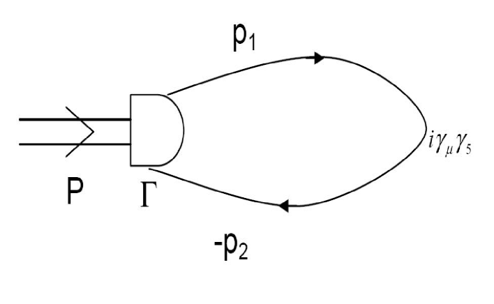
Figure 1:

References

- [1] S. Bhatnagar, S.-Y. Li, J. Phys.G 32, 949 (2006).
- [2] M.A. Ivanov, Yu.A. Kalinovsky, C.D. Roberts, Phys. Rev. D60, 034018 (1999).
- [3] C.D.Roberts, Nucl. Phys. A605, 475 (1996).
- [4] C.J. Burden, C.D. Roberts, M.J. Thomson, Phys. Lett. B371, 163 (1996).
- [5] R. Alkofer, L.V. Smekel, Phys. Rep.353, 281 (2001).
- [6] P.Maris, C.D.Roberts, Phys. Rev. C56, 3369 (1997).
- [7] D. S. Hwang and G. H. Kim, Phys. Rev. D 55 6944 (1997).
- [8] A.N. Mitra, S. Bhatnagar, Intl. J. Mod. Phys. A7, 121(1992).
- [9] J. Resag, C.R. Muenz, B.C. Metsch and H.R. Petry, Nucl.Phys. A578, 397 (1994).
- [10] S. Bhatnagar, D.S. Kulshreshtha, A.N. Mitra, Phys. Lett. B263, 485 (1991).
- [11] S. Bhatnagar, Intl. J. Mod. Phys. E 14, 909 (2005).
- [12] P.Maris, P.C.Tandy, Phys. Rev. C60, 055214 (1999).
- [13] R. Alkofer, P. Watson, H. Weigel, Phys. Rev. D65, 094026 (2002).
- [14] C. H. LLewellyn Smith, Ann. Phys. 53, 521 (1969).
- [15] S. Chakraborty et al., Prog. Part. Nucl. Phys. 22, 43 (1989).
- [16] Y.Nambu, G.Jona Lasino, Phys. Rev. 122, 345 (1961).
- [17] M.S.Bhagwat, M.A.Pichowsky, P.C.Tandy, Phys. Rev. D67, 054019 (2003).
- [18] A.N. Mitra, B.M. Sodermark, Nucl. Phys. A695, 328 (2001).
- [19] E. Follana et al (HPQCD and UKQCD), arXiv:0706.1726[hep-lat].
- [20] S.Narison, hep-ph/0202200.
- [21] S.Eidelman et al., (Particle Data Group), Phys. Lett. B592, 1, (2004).
- [22] BaBar and Belle Collaboration, http://utfit.roma1.infn.it/.
- [23] M.Artuso et al. (CLEO Collaboration), Phys. Rev. Lett. 95, 251801 (2005).