QCD corrections to single slepton production
at hadron colliders

Yu-Qi Chen¹, Tao Han^1,2,3, Zong-Guo Si⁴,

¹ Institute of Theoretical Physics, Academia Sinica, Beijing 100080, China

² Department of Physics, University of Wisconsin, Madison, WI 53706, USA

³ Department of Physics, Center for High-energy Physics Research, Tsinghua University, Beijing 100080, China

⁴ Department of Physics, Shandong University, Jinan Shandong 250100, China

E-Mail: ychen@itp.ac.cn, than@physics.wisc.edu, zgsi@sdu.edu.cn

Abstract
We evaluate the cross section for single slepton production at hadron colliders in supersymmetric theories with $R$-parity violating interactions to the next-to-leading order in QCD. We obtain fully differential cross section by using the phase space slicing method. We also perform soft-gluon resummation to all order in $\alpha_{s}$ of leading logarithm to obtain a complete transverse momentum spectrum of the slepton. We find that the full transverse momentum spectrum is peaked at a few GeV, consistent with the early results for Drell-Yan production of lepton pairs. We also consider the contribution from gluon fusion via quark-triangle loop diagrams dominated by the $b$-quark loop. The cross section of this process is significantly smaller than that of the tree-level process induced by the initial $b\bar{b}$ annihilation.

Keywords: QCD corrections, Resummation, Supersymmetry, R-parity

1 Introduction

The recent evidence of neutrino oscillation unambiguously indicates non-zero masses of neutrinos [1]. This poses a fundamental question: Whether or not the color and electrically neutral neutrinos are Majorana fermions, whose mass term violates the lepton number by two units. In general, lepton-number violating interactions of $\Delta L=1,2$ will induce a Majorana mass for neutrinos. Thus searching for the effects of lepton-number violation is of fundamental importance to establish the Majorana nature of the neutrinos and of significant implications for particle physics, nuclear physics and cosmology.

Weak scale supersymmetry (SUSY) remains to be a leading candidate for physics beyond the standard model (SM). While SUSY models often yield rich physics in the flavor sector, theories with $R$-parity violation may have lepton-number violating interactions and thus provide a Majorana mass for neutrinos [2, 3]. Proposals for searching for slepton production via $R$-parity violating interactions at hadron colliders already exist in the literature [4]. Experimental searches are being actively conducted at the Tevatron collider. Despite of the negative results [5], it is believed that it is conceivable to observe a signal of single slepton production at the Tevatron and the LHC if the interaction strengths is sufficiently large and is suitable for the neutrino mass generation [3, 6].

In this paper, we evaluate the cross section for a single slepton production in supersymmetric theories with $R$-parity violating interactions at the LHC to the next-to-leading order in QCD. We present fully differential cross sections by using the phase space slicing method. Our results, when overlapping, agree with an earlier calculation [7]. We also perform soft-gluon resummation to all order at leading log to obtain a complete transverse momentum spectrum. Our results here are consistent with a recent calculation [8]. We further consider the contribution with gluon fusion via quark-triangle diagrams, which could help probe the $R$-parity violating couplings involving $b$ quarks. We find that the cross section for this process is smaller than the process induced by initial $b\bar{b}$ state.

The paper is organized as follows: The cross sections of all single slepton production processes at leading order and next-to-leading order are presented in Sections 2 and 3 respectively, in a pedagogical manner. Numerical results at the Tevatron and the LHC are given and discussed in Section 3. The transverse momentum distribution of a slepton is calculated in Section 4. We further investigate the slepton production via gluon fusion through a heavy-quark loop in Section 5. Finally a short summary is given in Section 6.

2 Born Level results

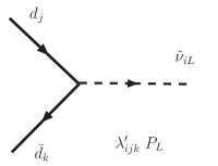
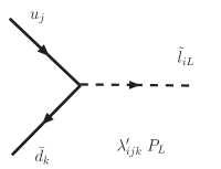
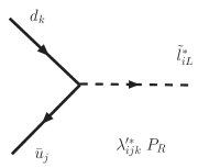
Figure 1: Feynman diagram for $\bar{q}^{\prime}(p_{1})+q(p_{2})\rightarrow\tilde{\ell}(q)$ in the $\not\!\!{R}$ SUSY model.

In this section, we set up our notation and the initial results for the Born-level cross sections. In $\not\!\!{R}$ SUSY models with a $\lambda^{\prime}$ coupling as shown in Fig. 1, a slepton or a sneutrino can be produced via quark anti-quark annihilation. The interaction couplings are proportional to $\lambda^{\prime}_{ijk}$ and are flavor-dependent. At the leading order, neglecting the flavor index, the generic process is

$$\bar{q}(p_{1})+q^{\prime}(p_{2})\rightarrow\tilde{\ell}(q),$$ (1)

where $p_{1}$, $p_{2}$ and $q$ denote the four momenta of the corresponding particles. The invariant amplitude for this process reads

$${\cal M}^{(0)}=\left\{\begin{array}[]{ll}-i\,\lambda^{\prime}\,\bar{v}(p_{1})\,P_{L}\,u(p_{2})&\mbox{for}\ \tilde{\nu},\ \tilde{\ell},\\ -i\,\lambda^{\prime*}\,\bar{v}(p_{1})\,P_{R}\,u(p_{2})&\mbox{for}\ \tilde{\nu}^{*},\ \tilde{\ell}^{*}.\end{array}\right.$$

with $P_{R,L}=(1\pm\gamma_{5})/2$. The Born-level cross section, after averaging over the initial spins and colors, is thus given by

$$\sigma_{Born}(\hat{s})=\frac{1}{N_{c}}\,\frac{1}{2\hat{s}}\,\int\frac{d^{d-1}q}{(2\pi)^{d-1}2q_{0}}\,\frac{1}{4}\,|{\cal M}^{(0)}|^{2}\,(2\pi)^{d}\,\delta^{d}(p_{1}+p_{2}-q)={{{\lambda^{\prime}}^{2}\pi}\over{4N_{c}\hat{s}}}\delta(1-\tau),$$ (2)

where $\hat{s}=(p_{1}+p_{2})^{2},\ \tau\,=\,m_{\tilde{\ell}}^{2}/\hat{s}$, and $d=4-2\epsilon$ is set to be 4 for the Born-level calculations.

3 Next-to-leading order QCD corrections

The leading order processes (1) receive QCD corrections. At the next leading order, they may arise from a real gluon emitting process, from one-loop virtual corrections, or from the gluon initiated process. As is well-known, although infrared (IR) divergences appear in each diagram individually, they cancel by adding them together. There are also collinear divergences arising from the fermion mass singularities in the real gluon emission and gluon splitting processes. They can be absorbed to the redefinition of the parton distribution functions. The ultraviolet (UV) divergences arising from the virtual corrections can be removed by renormalization of the coupling constants. Throughout this paper, we adopt dimensional regularization to regulate both the infrared and the ultraviolet divergences and use $\overline{\rm MS}$ scheme to carry out the renormalization and mass factorization.

3.1 Virtual corrections

We first calculate the contributions from the virtual corrections as shown in Fig. 2. With a straightforward calculation, we obtain the contribution to the cross section from the vertex diagram as

Figure 2: Feynman diagrams for virtual gluon corrections to $\bar{q}(p_{1})+q(p_{2})\rightarrow\tilde{\ell}(q)$.

$$\sigma_{vertex}(\hat{s})=\frac{C_{F}\alpha_{s}}{\pi}C_{\epsilon}\,\Big{(}\,-\frac{1}{\epsilon^{2}}+\frac{\pi^{2}}{2}-1\,\Big{)}\sigma_{Born}(\hat{s})\equiv K^{\prime}\ \sigma_{Born}(\hat{s})$$ (3)

$$C_{\epsilon}=\frac{1}{\Gamma(1-\epsilon)}\,\Big{(}\,\frac{4\pi\mu^{2}}{\hat{s}}\,\Big{)}^{\epsilon},\ \ C_{F}={N_{c}^{2}-1\over 2N_{c}}.$$ (4)

Note that the single $1/\epsilon$ pole is absent due to the cancellation between the IR and the UV poles.

The contribution from the one loop self-energy diagrams vanishes, since there is no energy scale involved for an on-shell massless quark, thus the virtual corrections are simply given by the vertex correction. Adding the contributions of the Born term and the virtual gluon corrections together, the cross section is

$$\sigma_{Born}\,+\,\sigma_{virtue} = {{\lambda^{\prime}}^{2}\,\pi\over 4N_{c}\,\hat{s}}\;\delta(1\,-\,\tau)\;\left(1+K^{\prime}\right)\;$$ (5)

$$\approx {{\lambda^{\prime}}_{R}^{2}\,\pi\over 4N_{c}\,\hat{s}}\;\delta(1\,-\,\tau)\;\left[\;(\,Z_{\lambda}\,Z_{2}^{-1}\,)^{2}+K^{\prime}\right]\;,$$

where ${\lambda^{\prime}}_{R}$ is the renormalized coupling constant, $Z_{{\lambda}}$ and $Z_{2}$ are the vertex and wave function renormalization constants extracted from the ultraviolet poles in the one-loop vertex and self-energy diagrams in Fig. 2, respectively, and are given in the ${\overline{\rm MS}}$ scheme by

$$Z_{{\lambda}}=1-\frac{\alpha_{s}}{4\pi\Gamma(1-\epsilon)}\ C_{F}(4\pi)^{\epsilon}\ \frac{4}{\epsilon},\quad Z_{2}=1-\frac{\alpha_{s}}{4\pi\Gamma(1-\epsilon)}\ C_{F}(4\pi)^{\epsilon}\ \frac{1}{\epsilon},$$ (6)

$${\lambda^{\prime}}_{R}={\lambda^{\prime}}\,Z_{\lambda}\,Z_{2}^{-1}\approx 1-\frac{\alpha_{s}}{4\pi\Gamma(1-\epsilon)}\ C_{F}(4\pi)^{\epsilon}\ \frac{3}{\epsilon}.$$ (7)

Combining the results above, we obtain the cross section with the Next-to-Leading Order (NLO) virtual corrections are

$$\sigma_{Born}+\sigma_{virtue}={{\lambda^{\prime}}_{R}^{2}\pi\over 4N_{c}\hat{s}}\delta(1-\tau)\left[1+\frac{C_{F}\alpha_{s}}{\pi}C_{\epsilon}\Big{(}-\frac{1}{\epsilon^{2}}-\frac{3}{2\epsilon}-\frac{3}{2}\ln\frac{\hat{s}}{\mu^{2}}+\frac{\pi^{2}}{2}-1\Big{)}\right].~{}$$ (8)

The infrared and collinear singularities are isolated by the double and single poles in $\epsilon$.

3.2 Real gluon emission

The real gluon emission processes

Figure 3: Feynman diagrams for $\bar{q}^{\prime}(p_{1})+q(p_{2})\rightarrow\tilde{l}(q)+g(k)$ in the $\not\!\!{R}$ SUSY model.

$$\bar{q}(p_{1})+q(p_{2})\rightarrow g(k)+\tilde{l}(q)\;,$$ (9)

as shown in Fig. 3 also contribute to the next leading order QCD corrections. The scattering matrix element and its square are

$${\cal M}^{a} = -i{\lambda^{\prime}}g_{s}\mu^{\epsilon}\,\epsilon^{\mu}(k)\bar{v}(p_{1})\,T^{a}\,\Big{(}\,\gamma_{\mu}\frac{\not{p}_{1}-\not{k}}{2p_{1}\cdot k}\,\frac{1+\gamma_{5}}{2}\,-\,\frac{1+\gamma_{5}}{2}\,\frac{\not{p}_{2}-\not{k}}{2p_{2}\cdot k}\,\gamma_{\mu}\Big{)}\,u(p_{2}),$$

$$|{\cal M}^{a}|^{2} = 16{\lambda^{\prime}}^{2}\,g_{s}^{2}\mu^{2\epsilon}\,N_{c}\,C_{F}\,{1\over\cos^{2}\theta}\,\left({1\over(1-\tau)^{2}}-{1\over 1-\tau}+{1-\epsilon\over 2}\right)\;,$$ (10)

where $\theta$ is the angle between the outgoing gluon and the initial anti-quark in the parton-level center mass frame system. The Lorentz invariant phase space integral reads:

$$\int\,d\,PS_{2}^{\epsilon} \;=\; \int\frac{d^{3-2\epsilon}k}{(2\pi)^{3-2\epsilon}\,2E_{g}}\,\frac{d^{3-2\epsilon}q}{(2\pi)^{3-2\epsilon}\,2q_{0}}\,\delta^{4-2\epsilon}(p_{1}+p_{2}-q-k)$$ (11)

$$\;=\; {(4\pi)^{-1+\epsilon}\over\Gamma(1-\epsilon)}\;{(1-\tau)^{1-2\epsilon}\over 2{\hat{s}}^{\epsilon}}\;\int^{\pi}_{0}\,d\theta\,\sin^{1-2\epsilon}\theta\;.$$

In order to retain kinematical distributions, we wish not to integrate out $\theta$. We adopt the phase space slicing method [9] to separate the IR and the collinear divergences. These singularities are isolated into the soft and collinear regions by two parameters $x_{min}$ and $\delta$, respectively, according to

$$E_{g}<\frac{\sqrt{\hat{s}}}{2}x_{min},$$ (12)

$$1-|\cos(\theta)|<\delta.$$ (13)

3.2.1 Soft region

In the soft region as defined by the gluon energy in Eq. (12), the contribution to the cross section is given by

$$\sigma_{soft} \;=\; \frac{1}{4N_{c}^{2}}\,\frac{1}{2\hat{s}}\,\int\,d\,PS_{2}^{\epsilon}\,|M^{a}|^{2}\,\Theta(\frac{\sqrt{\hat{s}}}{2}x_{min}-E_{g})\,$$ (14)

$$\;=\; \sigma_{Born}(\hat{s})\ \frac{C_{F}\alpha_{s}}{\pi}\,C_{\epsilon}\left(\frac{1}{\epsilon^{2}}-\frac{2\ln x_{min}}{\epsilon}+2\ln^{2}x_{min}-\frac{\pi^{2}}{6}\,\right),$$

We see that the above IR double pole just cancels that of the virtual correction in (8) as expected. The single pole is artificial and arises from the explicit cutoff.

3.2.2 Collinear region

The collinear region is constrained by Eq. (13) but in order to avoid double-counting, one must impose $E_{g}>\frac{\sqrt{\hat{s}}}{2}x_{min}$. Its contribution to the cross section is given by

$$\sigma_{col} = \frac{1}{4N_{c}^{2}}\,\frac{1}{2\hat{s}}\,\int\,d\,PS_{2}\,|M^{a}|^{2}\,\Theta(E_{g}-\frac{\sqrt{\hat{s}}}{2}x_{min})\,\,\Theta(\delta-1+|\cos(\theta)|)\,$$ (15)

$$= \sigma_{Born}(x\hat{s})\ \frac{C_{F}\alpha_{s}}{\pi}\,C_{\epsilon}\,\left(-\frac{2^{\epsilon}}{\epsilon}\,\right)\,(1-\epsilon\ln\delta)\int\limits_{0}^{1-x_{min}}\,dx\,\frac{1+x^{2}-\epsilon(1-x)^{2}}{(1-x)^{1+2\epsilon}},$$

where $1-x$ is the gluon energy-momentum fraction with respect to the parent quark defined as $k=(1-x)p_{1}~{}{\rm or}~{}k=(1-x)p_{2},$ depending on which quark the gluon is radiated from.

With the help of the “plus function”,

$$\Big{[}F(x)\Big{]}_{+}=\lim\limits_{\beta\rightarrow 0}\,\Big{[}\,\Theta(1-x-\beta)\,F(x)\,-\,\delta(1-x-\beta)\,\int\limits_{0}^{1-\beta}F(y)dy\,\Big{]}\,,$$ (16)

Eq. (15) can be rewritten as

$$\sigma_{col} = \frac{C_{F}\alpha_{s}}{\pi}C_{\epsilon}\ \Big{\{}\sigma_{Born}(\hat{s})\Big{[}\frac{2\ln x_{min}}{\epsilon}-2\ln^{2}x_{min}-2\ln x_{min}\ln\frac{\delta}{2}\Big{]}$$

$$+ \int\limits_{0}^{1}dx~{}\sigma_{Born}(x\hat{s})\Big{[}\left(-\frac{1}{\epsilon}+\ln\frac{\delta}{2}\right)\frac{1+x^{2}}{(1-x)_{+}}+(1-x)+2(1+x^{2})\Big{(}\frac{\ln(1-x)}{1-x}\Big{)}_{+}\Big{]}\Big{\}}.$$

Adding the contributions from leading term, virtual corrections, soft part, and the collinear part together, we have:

$$\sigma_{Born}\,+\,\sigma_{virtue}\,+\,\sigma_{soft}\,+\,\sigma_{col}$$

$$= {{\lambda^{\prime}}_{R}^{2}\,\pi\over 4N_{c}\,\hat{s}}\;\delta(1\,-\,\tau)\left[1+\frac{C_{F}\alpha_{s}}{\pi}\,C_{\epsilon}\,\Big{(}-\frac{3}{2\epsilon}-\frac{3}{2}\ln\frac{\hat{s}}{\mu^{2}}+\frac{\pi^{2}}{3}-1-2\ln x_{min}\ln{\delta\over 2}\Big{)}\,\right]$$

$$+ \frac{C_{F}\alpha_{s}}{\pi}C_{\epsilon}\int\limits_{0}^{1}dx~{}\sigma_{Born}(x\hat{s})\left[\Big{(}\ln\frac{\delta}{2}-\frac{1}{\epsilon}\Big{)}\frac{1+x^{2}}{(1-x)_{+}}+(1-x)+2(1+x^{2})\Big{(}\frac{\ln(1-x)}{1-x}\Big{)}_{+}\right].$$

The collinear divergence in $1/\epsilon$ is due to the massless approximation of the incoming quarks, and can be absorbed into the definition of parton densities. Within $\overline{\rm MS}$ scheme, the universal counter terms for the collinear subtraction are given by

$$\sigma_{col}^{CT} = \frac{C_{F}\alpha_{s}}{2\pi}\frac{1}{\Gamma(1-\epsilon)}\Big{(}\frac{4\pi\mu^{2}}{\mu_{F}^{2}}\Big{)}^{\epsilon}\Big{\{}\frac{3}{\epsilon}\sigma_{Born}(\hat{s})+\frac{2}{\epsilon}\int\limits_{0}^{1}dx\sigma_{Born}(x\hat{s})\frac{1+x^{2}}{(1-x)_{+}}\Big{\}}$$ (19)

$$= \frac{C_{F}\alpha_{s}}{\pi}\Big{[}\frac{C_{\epsilon}}{\epsilon}+\ln\frac{\hat{s}}{\mu_{F}^{2}}\Big{]}\,\Big{[}\frac{3}{2}\sigma_{Born}(\hat{s})+\int dx\,\frac{1+x^{2}}{(1-x)_{+}}\sigma_{Born}(x\hat{s})\,\Big{]},$$

where $\mu_{F}$ is the factorization scale. Adding (3.2.2) and (19) together and integrating over $\sigma_{Born}(x\hat{s})={\lambda^{\prime}}_{R}^{2}\,\pi/(4N_{c}\,\hat{s})\delta(x-\tau)$, we obtain

$$\sigma_{Born}\,+\,\sigma_{virtue}\,+\,\sigma_{soft}\,+\,\sigma_{col}\,+\,\sigma_{col}^{CT}$$ (20)

$$= {{\lambda^{\prime}}_{R}^{2}\,\pi\over 4N_{c}\,\hat{s}}\;\delta(1\,-\,\tau)\;\left[\;1\;+\;\frac{C_{F}\alpha_{s}}{\pi}\,\Big{(}\,-\frac{3}{2}\ln\frac{\mu^{2}_{F}}{\mu^{2}}\,+\,\frac{\pi^{2}}{3}-1-2\ln x_{min}\ln{\delta\over 2}\,\Big{)}\,\right]\;$$

$$+ \frac{C_{F}\alpha_{s}}{\pi}\ {{\lambda^{\prime}}_{R}^{2}\,\pi\over 4N_{c}\,\hat{s}}\left[\,(\ln\frac{\delta}{2}+\ln{\hat{s}\over\mu^{2}_{F}})\frac{1+\tau^{2}}{(1-\tau)_{+}}+(1-\tau)+2(1+\tau^{2})\,\Big{(}\,\frac{\ln(1-\tau)}{1-\tau}\Big{)}_{+}\,\right].~{}\quad$$

Obviously, the infrared and the collinear divergences are cancelled as expected. We note, however, there are still explicit dependences on the hard cutoff parameters $x_{min}$ and $\delta$.

3.2.3 Hard scattering

The tree-level $2\to 2$ processes as in Eq. (9) contribute to the order of $\alpha_{s}$. The region of hard scattering is constrained by $E_{g}>\frac{\sqrt{\hat{s}}}{2}x_{min}$ and $1-|\cos(\theta)|>\delta$. Since the contribution to the cross section from this region is finite, we can take $\epsilon=0$ in the calculation. In fact, it is a regularized $2\to 2$ “resolvable” process and the differential cross section is written as

$$\sigma_{2\to 2} = \frac{1}{4N_{c}^{2}}\,\frac{1}{2\hat{s}}\int dPS_{2}|{\cal M}^{a}|^{2}~{}\Theta(1-\delta-|\cos\theta|)\Theta(E_{g}-\frac{\sqrt{\hat{s}}}{2}x_{min})$$ (21)

$$= \frac{C_{F}\alpha_{s}{\lambda^{\prime}}^{2}}{4N_{c}\hat{s}}\int d\cos\theta\ \Theta(1-\delta-|\cos\theta|)\Theta(1-x_{min}-\tau)\frac{1}{1-\cos^{2}\theta}\ \frac{1+\tau^{2}}{1-\tau}.\quad~{}$$

It is Eqs. (20) and (21) that give the complete cross section for the $q\bar{q}$ initiated process at the order of $\alpha_{s}$.

The dependence on the cutoff parameters $x_{min}$ and $\delta$ are explicit in these two equations, reflecting the arbitrariness of our definition of “soft” and “collinear” regions. However, the summed total cross section should be independent of those choices. To see this feature, we choose to integrate over $\theta$ and have

$$\sigma_{2\to 2} = -\,\frac{C_{F}\alpha_{s}{\lambda^{\prime}}^{2}}{4N_{c}\hat{s}}\,\Theta(1-x_{min}-\tau)\,\frac{1+\tau^{2}}{1-\tau}\,\ln\frac{\delta}{2}$$ (22)

$$= \frac{C_{F}\alpha_{s}{\lambda^{\prime}}^{2}}{4N_{c}\hat{s}}\,\left[\,-\ln\frac{\delta}{2}\,\frac{1+\tau^{2}}{(1-\tau)_{+}}\,+\,2\ln\frac{\delta}{2}\,\ln x_{min}\,\delta(1-\tau)\,\right],$$

where the “plus-function” of Eq.(16) in the limit $x_{min}\rightarrow 0$

$$\frac{1+\tau^{2}}{1-\tau}\Theta(1-x_{min}-\tau)\;=\;\frac{1+\tau^{2}}{(1-\tau)_{+}}\,-\,2\ln x_{min}\,\delta(1-\tau)$$ (23)

has been used.

Putting (20) and (22) together, we obtain the total cross section of $q\bar{q}$ processes to the next leading order

$$\hat{\sigma}_{q\bar{q}} = \sigma_{Born}+\sigma_{vir}+\sigma_{col}+\sigma_{col}^{CT}+\sigma_{2\to 2}$$ (24)

$$= {{\lambda^{\prime}}_{R}^{2}\,\pi\over 4N_{c}\hat{s}}\,\left\{\,\delta(1-\tau)\;+\;\frac{C_{F}\alpha_{s}}{\pi}\,\left[\,\left(\,\frac{3}{2}\ln\frac{\mu^{2}}{\mu_{F}^{2}}+\frac{\pi^{2}}{3}-1\,\right)\,\delta(1-\tau)\,\right.\right.$$

$$\,+\,\left.\left.\frac{1+\tau^{2}}{(1-\tau)_{+}}\,\ln\frac{\hat{s}}{\mu_{F}^{2}}\,+\,(1-\tau)\,+\,2(1+\tau^{2})\,\left(\,\frac{\ln(1-\tau)}{1-\tau}\,\right)_{+}\,\right]\;\right\},$$

where we have verified the independence of the cutoff parameters.

3.3 Gluon-initiated process

In next leading order, the gluon-initiated process

$$g(p_{1})+q(p_{2})\rightarrow\tilde{l}(q)+q(k),$$ (25)

also contributes to the cross section. Two Feynman diagrams contributing to the process are shown in Fig. 4. With the Feynman rule given in Fig. 1, the cross section can be written as

$$\tilde{\sigma}_{res}=\frac{1}{4N_{c}(N_{c}^{2}-1)}\frac{1}{2\hat{s}}\int|\tilde{\cal M}|^{2}~{}\Theta(1-\delta-|\cos\theta|)~{}dPS_{2}^{\epsilon}$$ (26)

where

$$\tilde{\cal M}^{a} = -i{\lambda^{\prime}}g_{s}\mu^{\epsilon}\,\epsilon^{\mu*}(p_{1})\,\bar{u}(k)\,T^{a}\,\Big{(}\,P_{R}\,\frac{\not{p}_{1}+\not{p}_{2}}{\hat{s}}\gamma_{\mu}\,+\,\gamma_{\mu}\frac{\not{p}_{1}-\not{k}}{2p_{1}\cdot k}\,P_{R}\,\Big{)}\,u(p_{2})$$ (27)

$$|\tilde{\cal M}^{a}|^{2} = {\lambda^{\prime}}^{2}g_{s}^{2}N_{c}C_{F}\,\left[\,\frac{4}{1-\cos\theta}\,\left(\,\frac{1}{1-\tau}-2\tau\,\right)\,-\,(\,3+\cos\theta\,)\,(\,1-\tau\,)\,\right].$$ (28)

Figure 4: Feynman diagrams for $g(p_{1})+q(p_{2})\rightarrow\tilde{l}(q)+q(k)$ in the $\not\!\!{R}$ SUSY model.

There are collinear divergences but no infrared divergence for a gluon splitting to $q\bar{q}$. Similar to the case of $q\,\bar{q}\,\to\,\tilde{l}\,g$ process, we can separate the contributions to the cross section into collinear part and hard by imposing a cutoff $1-|\cos\theta|=\delta$ on the phase space, where $\theta$ is the angle between the moving direction of the initial gluon and that of the outgoing quark. Integrating over $\theta$ within $1-|\cos\theta|<\delta$, we obtain the collinear part:

$$\tilde{\sigma}_{col} = -\frac{\alpha_{s}}{4\pi}C_{\epsilon}\int\limits_{0}^{1}dx~{}\sigma_{Born}(x\hat{s})\,\frac{2^{\epsilon}}{\epsilon}\,\Big{(}1-\epsilon\ln\delta\Big{)}\,\frac{x^{2}+(1-x)^{2}}{(1-\epsilon)(1-x)^{2\epsilon}}$$ (29)

$$= \frac{\alpha_{s}}{4\pi}C_{\epsilon}\ {{\lambda^{\prime}}^{2}\,\pi\over 4N_{c}\hat{s}}\ \Big{\{}1+\Big{[}\tau^{2}+(1-\tau)^{2}\Big{]}\,\Big{[}-\frac{1}{\epsilon}+\ln\,\frac{\delta}{2}+2\ln(1-\tau)-1\Big{]}\Big{\}},$$

where $x$ is defined as $k=(1-x)p_{1}$.

Within $\overline{\rm MS}$ scheme, the universal collinear counter term is given by

$$\tilde{\sigma}_{col}^{CT} = \frac{\alpha_{s}}{4\pi}\frac{1}{\Gamma(1-\epsilon)}\Big{(}\frac{4\pi\mu^{2}}{\mu_{F}^{2}}\Big{)}^{\epsilon}\frac{1}{\epsilon}\int\limits_{0}^{1}\,dx\sigma_{Born}(x\hat{s})~{}\Big{\{}x^{2}+(1-x)^{2}\Big{\}}$$ (30)

$$= \frac{\alpha_{s}}{4\pi}\Big{(}\frac{C_{\epsilon}}{\epsilon}+\ln\frac{\hat{s}}{\mu_{F}^{2}}\Big{)}\,{{\lambda^{\prime}}^{2}\,\pi\over 4N_{c}\hat{s}}\ \Big{[}\tau^{2}+(1-\tau)^{2}\Big{]}.$$

Then we have

$$\tilde{\sigma}_{col}+\tilde{\sigma}_{col}^{CT} = \frac{{\lambda^{\prime}}^{2}\alpha_{s}}{16N_{c}\hat{s}}\,\Big{\{}1+\Big{[}\tau^{2}+(1-\tau)^{2}\Big{]}\,\Big{[}\ln\frac{\delta\ \hat{s}}{2\ \mu_{F}^{2}}+2\ln(1-\tau)-1\Big{]}\Big{\}}.$$ (31)

The “resolvable” $2\to 2$ cross section is free from collinear singularity and can be calculated in 4-dimension

$$\tilde{\sigma}_{2\to 2} = \frac{{\lambda^{\prime}}^{2}\,\alpha_{s}}{16N_{c}\hat{s}}\,\int\limits_{-1}^{1-\delta}\Big{\{}\frac{1}{1-\cos\theta}\,\Big{[}(1-\tau)^{2}+\tau^{2}\Big{]}-\frac{3+\cos\theta}{4}\,(1-\tau)^{2}\Big{\}}\,d\cos\theta$$ (32)

$$= \frac{{\lambda^{\prime}}^{2}\,\alpha_{s}}{16N_{c}\hat{s}}\,\Big{\{}-\Big{[}(1-\tau)^{2}+\tau^{2}\Big{]}\,\ln\frac{\delta}{2}-\frac{3}{2}\,(1-\tau)^{2}\Big{\}}.$$

The final result of the total cross section is independent of the cutoff parameters and is given by

$$\hat{\sigma}_{gq} = \hat{\sigma}_{g\bar{q}}=\tilde{\sigma}_{col}+\tilde{\sigma}_{col}^{CT}+\tilde{\sigma}_{2\to 2}$$ (33)

$$= \frac{{\lambda^{\prime}}^{2}\alpha_{s}}{16N_{c}\hat{s}}\,\left\{\Big{[}\tau^{2}+(1-\tau)^{2}\Big{]}\,\Big{[}\ln\frac{\hat{s}}{\mu_{F}^{2}}+2\ln(1-\tau)\Big{]}+\frac{(1-\tau)(7\tau-3)}{2}\right\}.$$

We find that our analytical results at NLO QCD are in agreement with those in the literature [7].

3.4 Total cross sections at hadron colliders

Given the leading and the next leading order cross sections of the subprocesses above, we now investigate the total cross sections of the slepton production at hadron colliders such as the Tevatron and the LHC at the next leading order.

The total cross sections are formally given by the QCD factorization formula as

$$\sigma(S)=\sum_{i,j}\int dx_{1}dx_{2}\;f_{i}(x_{1},\mu)\,f_{j}(x_{2},\mu)\hat{\sigma}_{ij}(x_{1}x_{2}S,\mu),$$ (34)

where $f_{i,j}$ are parton distribution functions (PDF) and $i,j$ sum over all possible types of partons contributing to the subprocesses, $\mu$ is the factorization scale. In our numerical calculations, we consistently take to the leading and the next leading order parton distribution functions, CTEQ6L and CTEQ6.1M parton distribution functions [10] for the leading order for the next leading order calculations, respectively and take $\mu$ to be the slepton mass.

A useful quantity to describe the contributions from the next leading order corrections is the $K$-factor which is defined as the ratio of the next leading total cross section to the leading order one, $K\equiv\sigma_{NLO}/{\sigma_{LO}}$. We will show the numerical results of ${\sigma_{LO}}$, $\sigma_{NLO}$, and the corresponding $K$-factor for various processes at the Tevatron and the LHC energies.

Figure 5: Cross sections at the LO (dashed line) and the NLO (solid line) and their corresponding $K$-factor related to ${\lambda^{\prime}}_{i11}$ for $d\bar{d}\rightarrow\tilde{\nu}_{i}+X$ shown in (a) and (c), and $u\bar{d}(d\bar{u})\rightarrow\tilde{\ell}^{+}(\tilde{\ell}^{-})$ in (b) and (d) at the Tevatron ($\sqrt{s}=2$ TeV) and the LHC ($\sqrt{s}=14$ TeV).

To keep our presentation model-independent, we pull out the overall $\not\!\!{R}$ coupling ${\lambda^{\prime}}_{ijk}^{2}$ when showing the cross sections unless specified otherwise. We remind the reader that the last two indices ($j,k$) refer to the generation of quark partons and the first index ($i$) is for the slepton. Thus our results are formally applicable to any flavor of the sleptons, and are given in Figs. 5$-$10:

$${\rm Fig.~{}\ref{csnlol11}}:\quad d\bar{d}\rightarrow\tilde{\nu}_{i},\ \ {\rm and}\ \ u\bar{d}\ (d\bar{u})\rightarrow\tilde{\ell}^{+}\ (\tilde{\ell}^{-}),\quad{\rm for\ probing}\ \lambda^{\prime}_{i11}.$$

$${\rm Fig.~{}\ref{csnlol12}}:\quad d\bar{s},\ s\bar{d}\rightarrow\tilde{\nu}_{i},\ \ {\rm and}\ \ u\bar{s}\ (s\bar{u})\rightarrow\tilde{\ell}^{+}\ (\tilde{\ell}^{-}),\quad{\rm for\ probing}\ \lambda^{\prime}_{i12}.$$

$${\rm Fig.~{}\ref{csnlol13}}:\quad d\bar{b},\ b\bar{d}\rightarrow\tilde{\nu}_{i},\ \ {\rm and}\ \ u\bar{b}\ (b\bar{u})\rightarrow\tilde{\ell}^{+}\ (\tilde{\ell}^{-}),\quad{\rm for\ probing}\ \lambda^{\prime}_{i13}.$$

$${\rm Fig.~{}\ref{csnlol22}}:\quad s\bar{s}\rightarrow\tilde{\nu}_{i},\ \ {\rm and}\ \ c\bar{s}\ (s\bar{c})\rightarrow\tilde{\ell}^{+}\ (\tilde{\ell}^{-}),\quad{\rm for\ probing}\ \lambda^{\prime}_{i22}.$$

$${\rm Fig.~{}\ref{csnlol23}}:\quad s\bar{b},\ b\bar{s}\rightarrow\tilde{\nu}_{i},\ \ {\rm and}\ \ c\bar{b}\ (b\bar{c})\rightarrow\tilde{\ell}^{+}\ (\tilde{\ell}^{-}),\quad{\rm for\ probing}\ \lambda^{\prime}_{i23}.$$

$${\rm Fig.~{}\ref{csnlol33}}:\quad b\bar{b}\rightarrow\tilde{\nu}_{i},\quad{\rm for\ probing}\ \lambda^{\prime}_{i33}.$$

It is seen that the production rate of the slepton is larger than that of sneutrino, due to the parton luminosity difference and the charged state counting. While the production cross sections for these processes at the LHC energies are larger than that at the Tevatron energies by about one order of magnitude at $m_{\tilde{\ell}}\mathrel{\raise 1.29167pt\hbox{$<$\kern-7.5pt\lower 4.30554pt\hbox{$\sim$}}}200$ GeV, and about two orders of magnitude at $m_{\tilde{\ell}}\mathrel{\raise 1.29167pt\hbox{$>$\kern-7.5pt\lower 4.30554pt\hbox{$\sim$}}}700$ GeV. we see that the NLO QCD corrections and the $K$-factors are largely reflecting ratio of the parton distributions at different scale and $x$-values, and are of the following features.

• At the LHC, the QCD corrections are rather stable and increasing monotonically versus $m_{\tilde{\ell}}$. The $K$-factors are typically around $1.2-1.4$, except that the range becomes slightly larger when more sea quarks are involved.

• At the Tevatron, the $K$-factor is around $1.1-1.5$ when the valence quarks dominate as for $\lambda_{i11}$ in Fig. 5. For other channels, the QCD corrections are less stable. The $K$-factors can be larger than a factor of two at high masses or large $x$-values where the sea quark distributions fall quickly. This effect was also observed in [7].

Figure 6: Cross sections at the LO (dashed line) and the NLO (solid line) and their corresponding $K$-factor related to ${\lambda^{\prime}}_{i12}$ for $d\bar{s}(s\bar{d})\rightarrow\tilde{\nu}_{i}+X$ shown in (a) and (c), and $u\bar{s}(s\bar{u})\rightarrow\tilde{\ell}^{+}(\tilde{\ell}^{-})$ in (b) and (d) at the Tevatron and the LHC.

Figure 7: Cross sections at the LO (dashed line) and the NLO (solid line) and their corresponding $K$-factor related to ${\lambda^{\prime}}_{i13}$ for $d\bar{b}(b\bar{d})\rightarrow\tilde{\nu}_{i}+X$ shown in (a) and (c), and $u\bar{b}(b\bar{u})\rightarrow\tilde{\ell}^{+}(\tilde{\ell}^{-})$ in (b) and (d) at the Tevatron and the LHC.

Figure 8: Cross sections at the LO (dashed line) and the NLO (solid line) and their corresponding $K$-factor related to ${\lambda^{\prime}}_{i22}$ for $s\bar{s}\rightarrow\tilde{\nu}_{i}+X$ shown in (a) and (c), and $c\bar{s}(s\bar{c})\rightarrow\tilde{\ell}^{+}(\tilde{\ell}^{-})$ in (b) and (d) at the Tevatron and the LHC.

Figure 9: Cross sections at the LO (dashed line) and the NLO (solid line) and their corresponding $K$-factor related to ${\lambda^{\prime}}_{i23}$ for $s\bar{b}(b\bar{s})\rightarrow\tilde{\nu}_{i}+X$ shown in (a) and (c), and $c\bar{b}(b\bar{c})\rightarrow\tilde{\ell}^{+}(\tilde{\ell}^{-})$ in (b) and (d) at the Tevatron and the LHC.

Figure 10: (a) Cross sections related to ${\lambda^{\prime}}_{i33}$ for $b\bar{b}\rightarrow\tilde{\nu}_{i}+X$ at the LO (dashed line) and the NLO (solid line) at the Tevatron and the LHC and (b) their corresponding $K$-factor.

3.5 Event rates and signal detection at hadron colliders

So far we have not specified the values for the $\not\!\!{R}$ couplings. There are stringent bounds on them from low energy data. We consider the strongest constraints for $\lambda^{\prime}_{ijk}$ determined from the charge and neutral currents as summarized in a recent review [6], and calculate the corresponding cross sections for the slepton and sneutrino production. The results are listed in Table 1. It is known that the bounds on the couplings of the lighter generation sleptons are significantly tighter than the heavier generations. The production rates related to $\tilde{\tau}$ and $\tilde{\nu}_{\tau}$ could be much larger than that of the other sleptons and sneutrinos because of the possibly larger couplings. For illustration, we have considered the mass range of $m_{\tilde{\ell}}=150-500$ GeV. The production rates are sizable, given the fact that the designed high luminosity at the LHC may reach 100 fb^-1 annually.

As for the final state identification of the signal, it is likely to go through the $R$-parity conserving decays as the $\lambda^{\prime}s$ are expected to be small. Thus the clean decay modes with at least one charged lepton may include

$$\tilde{\ell}^{\pm} \to \tilde{\chi}^{0}\ell^{\pm},\ \tilde{\chi}^{\pm}\nu;$$ (35)

$$\tilde{\nu} \to \tilde{\chi}^{\pm}\ell^{\pm}.$$ (36)

The feasibility for the signal identification has been studied extensively in the literature based on leading order cross sections, and we thus refer the readers to a review article [6] and references therein. Especially, the appropriate coupling ranges for neutrino mass generation can be tested in the collider experiments [3]. It is also interesting to note that for a sizable coupling $\lambda^{\prime}_{i33}$, it may lead to an observable heavy quark final state $b\bar{b}$, but not $t\bar{t}$.

$\lambda^{\prime}$	Upper	$\sigma$ for $m_{\tilde{\ell}}=150-500$ GeV
	bounds		Tevatron (pb)	LHC (pb)
$\lambda^{\prime}_{111}$	0.02	$\tilde{\nu}_{e}$	1.0–0.01	10–0.21
		$\tilde{e}$	3.6–0.03	25–0.55
$\lambda^{\prime}_{211}$	0.06	$\tilde{\nu}_{\mu}$	9.8–0.05	91–1.9
		$\tilde{\mu}$	33–0.28	221–5.0
$\lambda^{\prime}_{311}$	0.12	$\tilde{\nu}_{\tau}$	36–0.21	363–7.6
		$\tilde{\tau}$	131–1.1	885–20
$\lambda^{\prime}_{112}$	0.02	$\tilde{\nu}_{e}$	0.59–$10^{-3}$	12–0.21
		$\tilde{e}$	1.37–3$\cdot 10^{-3}$	22–0.42
$\lambda^{\prime}_{212}$	0.06	$\tilde{\nu}_{\mu}$	5.3–0.01	110–1.9
		$\tilde{\mu}$	12–0.03	201–3.7
$\lambda^{\prime}_{312}$	0.12	$\tilde{\nu}_{\tau}$	21–0.03	442–7.5
		$\tilde{\tau}$	49–0.10	805–15
$\lambda^{\prime}_{113}$	0.02	$\tilde{\nu}_{e}$	0.33–5$\cdot 10^{-4}$	8.4–0.15
		$\tilde{e}$	0.40–7$\cdot 10^{-4}$	9.4–0.17
$\lambda^{\prime}_{213}$	0.06	$\tilde{\nu}_{\mu}$	3.0–5 $\cdot 10^{-3}$	76–1.3
		$\tilde{\mu}$	3.6–0.01	85–1.6
$\lambda^{\prime}_{313}$	0.12	$\tilde{\nu}_{\tau}$	12–0.02	302–5.8
		$\tilde{\tau}$	14–0.03	339–6.3
$\lambda^{\prime}_{122}$	0.21	$\tilde{\nu}_{e}$	7.5–4$\cdot 10^{-3}$	333–4.0
		$\tilde{e}$	9.1–5$\cdot 10^{-3}$	526–5.7
$\lambda^{\prime}_{222}$	0.21	$\tilde{\nu}_{\mu}$	7.5–4$\cdot 10^{-3}$	333–4.0
		$\tilde{\mu}$	9.1–5$\cdot 10^{-3}$	526–6.0
$\lambda^{\prime}_{322}$	0.52	$\tilde{\nu}_{\tau}$	46–0.03	2043–24
		$\tilde{\tau}$	56–0.03	3223-35
$\lambda^{\prime}_{123}$	0.21	$\tilde{\nu}_{e}$	2.4–1$\cdot 10^{-3}$	162–1.8
		$\tilde{e}$	2.8–2$\cdot 10^{-3}$	245–2.5
$\lambda^{\prime}_{223}$	0.21	$\tilde{\nu}_{\mu}$	2.4–1$\cdot 10^{-3}$	162–1.8
		$\tilde{\mu}$	2.8–2$\cdot 10^{-3}$	245–2.5
$\lambda^{\prime}_{323}$	0.52	$\tilde{\nu}_{\tau}$	15–0.01	992–11
		$\tilde{\tau}$	17–0.01	1502–15
$\lambda^{\prime}_{133}$	0.18	$\tilde{\nu}_{e}$	0.52–3$\cdot 10^{-4}$	53–0.56
$\lambda^{\prime}_{233}$	0.45	$\tilde{\nu}_{\mu}$	3.3–2$\cdot 10^{-3}$	333–3.5
$\lambda^{\prime}_{333}$	0.58	$\tilde{\nu}_{\tau}$	5.4–3$\cdot 10^{-3}$	553–5.8

Table 1: Upper bounds on $\lambda^{\prime}$ in units of $(m_{\tilde{\ell}}/100\ \rm GeV)^{-2}$ and the corresponding cross sections for slepton and sneutrino production.

4 Transverse momentum distributions and soft gluon resummation

With the differential cross sections obtained in Sec. 3, we can also calculate the transverse momentum ($p_{T}$) distribution of the produced slepton associated with a hard parton in the final state. In considering the $p_{T}$ distribution, two different energy scales are involved, i.e., $p_{T}$ and $m_{\tilde{\ell}}$. When $p_{T}$ is comparable to $m_{\tilde{\ell}}$ or higher, fixed order perturbation theory gives sufficiently accurate results. However, when $p_{T}\ll m_{\tilde{\ell}}$, large logarithmic terms such as $(\alpha_{s}\ln^{2}p_{T}/m_{\tilde{\ell}})^{n}$ arise at fixed order perturbation calculations and need to be resummed in order to obtain reliable predictions.

Following the standard procedure [11], we first obtain the leading order asymptotic cross section in the limit of small transverse momentum

$$\frac{d\sigma^{asym}}{dp_{T}~{}dy} = \sigma_{Born}\,\frac{\alpha_{s}}{\pi}\frac{1}{S\,p_{T}}\Big{\{}\Big{(}A\ln\frac{m_{\tilde{\ell}}^{2}}{p_{T}^{2}}+B\Big{)}f_{q}(x_{1}^{0})f_{\bar{q}}(x_{2}^{0})+(f_{\bar{q}}\otimes P_{\bar{q}\leftarrow\bar{q}})(x_{1}^{0})f_{q}(x_{2}^{0})$$ (37)

$$+(f_{g}\otimes P_{\bar{q}\leftarrow g})(x_{1}^{0})f_{q}(x_{2}^{0})\Big{\}}+\Big{(}x_{1}^{0}\leftrightarrow x_{2}^{0}\Big{)},$$

$$(f\otimes g)(x) \equiv \int\limits_{x}^{1}f(y)\,g(\frac{x}{y})dy,\ \ P_{\bar{q}\leftarrow\bar{q}}(x)=\frac{4}{3}\Big{[}\frac{1+x^{2}}{1-x}\Big{]}_{+},\ \ P_{\bar{q}\leftarrow g}(x)=\frac{1}{2}\Big{[}x^{2}+(1-x)^{2}\Big{]}.$$

where $y$ is the rapidity of the parton c.m. system, $x^{0}_{1,2}\equiv e^{\pm y}m_{\tilde{\ell}}/\sqrt{S}$, and the expansion coefficients relevant for the leading-log resummation are determined to be $A=A^{(1)}=2C_{F},\ B=B^{(1)}=-3C_{F}$.

The resummed differential cross section can be expressed as the integral over the impact parameter $b$:

$$\frac{d\sigma^{resum}}{dp_{T}dy} = \sigma_{Born}\frac{2P_{T}}{S}\int\limits_{0}^{\infty}db\,\frac{b}{2}\,J_{0}(bp_{T})W(b),$$ (38)

$$W(b) = \exp\left[\,-\int\limits_{{b_{0}^{2}}/{b_{*}^{2}}}^{m_{\tilde{l}}^{2}}\,\frac{dq^{2}}{q^{2}}\,\frac{\alpha_{s}(q^{2})}{2\pi}\,\Big{(}A\ln\frac{m_{\tilde{l}}^{2}}{p_{T}^{2}}+B\Big{)}\,\right]\,S_{np}f_{q}(x_{1}^{0})f_{\bar{q}}(x_{2}^{0})+\Big{(}x_{1}^{0}\leftrightarrow x_{2}^{0}\Big{)},$$

$$S_{np} = \exp\left(-b^{2}g_{1}-b^{2}g_{2}\,\ln\,\frac{b_{max}m_{\tilde{l}}}{2}\,\right)\,,$$

$$b_{*} = \frac{b}{1+b^{2}/b_{max}^{2}},~{}~{}g_{1}=0.24\ {\rm GeV}^{2},~{}~{}g_{2}=0.34\ {\rm GeV}^{2},~{}~{}b_{max}=(1\ {\rm GeV})^{-1},$$ (39)

where the parameters are taken from Ref. [12] based on a fit to the Tevatron Drell-Yan data. Including an ansaz for matching between the resummed low momentum region and the perturbative high momentum region, the full transverse momentum distribution is thus expressed as

$$\frac{d\sigma^{full}}{dp_{T}} = \int dy\,\left[\,\frac{d\sigma^{pert}}{dp_{T}dy}+f(p_{T})\,\left(\,\frac{d\sigma^{resum}}{dp_{T}dy}-\frac{d\sigma^{asym}}{dp_{T}~{}dy}\,\right)\,\right],$$ (40)

$$f(p_{T}) = \frac{1}{1+(p_{T}/m_{\tilde{l}})^{4}}.$$ (41)

We must emphasize that the ad-hoc function $f(p_{T})$ is somewhat arbitrary and it reflects our ignorance for the distribution in the region $p_{T}\sim m_{\tilde{l}}$. The only way to reduce this arbitrariness would be to include higher order calculations in both perturbative and resummed regimes.

Figure 11: Distributions of ${d\sigma^{full}}/{dp_{T}}$ (solid line), ${d\sigma^{pert}}/{dp_{T}}$ (dashed line), ${d\sigma^{resum}}/{dp_{T}}$ (dash-dotted line) and ${d\sigma^{asym}}/{dp_{T}}$ (dotted line) for sneutrino production at (a) Tevatron ($\sqrt{s}=2$ TeV), and (b) LHC ($\sqrt{s}=14$ TeV).

Here as an example, we show the results of $d\bar{d}\rightarrow\tilde{\nu}_{i}+X$ in Fig. 11, with $m_{\tilde{\nu}_{i}}=100$ and $200$ GeV at Tevatron ($\sqrt{s}=2$ TeV) and LHC ($\sqrt{s}=14$ TeV). The results are obtained by using CTEQ6.1M. The distribution at small $p_{T}$ is dominated by the resummed part, while at large $p_{T}$, the contributions are mostly from the perturbative part. For the $\frac{d\sigma^{full}}{dp_{T}}$, the peak is between $2$ and $3$ GeV. The results for the other $q\bar{q}^{\prime}\rightarrow\tilde{\ell}+X$ processes are similar.

5 The $gg\rightarrow\tilde{\nu}$ Process

Because of the large gluon luminosity at high energies, one may consider the gluon fusion contribution to the single slepton production via quark triangle loops

$$g(p_{1})+g(p_{2})\rightarrow\tilde{\nu}(q).$$ (42)

Figure 12: Feynman diagram for $g(p_{1})+g(p_{2})\rightarrow\tilde{\nu}(q)$ via quark loops.

This process comes from diagrams shown in Fig. 12, and the corresponding amplitude is

$${\cal M} = -{\lambda^{\prime}}\,g_{s}^{2}\,\frac{\delta_{ab}}{2}\,\epsilon^{\mu}(p_{1})\,\epsilon^{\nu}(p_{2})\,{M}_{\mu\nu},$$ (43)

$${M}_{\mu\nu} = \int\frac{d^{4}l}{(2\pi)^{4}}\frac{N_{\mu\nu}}{[l^{2}-m_{q}^{2}+i\epsilon][(l+p_{1})^{2}-m_{q}^{2}+i\epsilon][(l+p_{1}+p_{2})^{2}-m_{q}^{2}+i\epsilon]},$$

$$N_{\mu\nu} = Tr\Big{\{}\gamma_{\mu}(\not{l}+m_{q})\frac{1+\gamma_{5}}{2}(\not{l}+\not{p}_{1}+\not{p}_{2}+m_{q}]\gamma_{\nu}[\not{l}+\not{p}_{1}+m_{q}]\Big{\}}$$

$$-Tr\Big{\{}\gamma_{\mu}(\not{l}+\not{p}_{1}-m_{q})\gamma_{\nu}[\not{l}+\not{p}_{1}+\not{p}_{2}-m_{q}]\frac{1+\gamma_{5}}{2}(\not{l}-m_{q})\Big{\}}\;.$$

With a straightforward calculation, we obtain the cross section of the subprocess:

$$\hat{\sigma}_{gg} = \frac{1}{2\hat{s}}\frac{1}{4(N_{c}^{2}-1)^{2}}\int|{\cal M}|^{2}\frac{d^{3}q}{(2\pi)^{3}2q^{0}}(2\pi)^{4}\delta^{4}(p_{1}+p_{2}-q)$$

$$= \frac{\alpha_{s}^{2}{\lambda^{\prime}}^{2}}{16\pi\,(N_{c}^{2}-1)}\frac{m_{q}^{2}}{\hat{s}^{2}}\,\Big{\{}[(\hat{s}-2m_{q}^{2})^{2}+4m_{q}^{4}]|C_{0}|^{2}+2+(8m^{2}_{q}-2\hat{s})Re[C_{0}]\Big{\}}~{}\delta(1-\tau),$$

where $C_{0}$ is the loop integral and is given by

$$C_{0} = \int\frac{d^{4}l}{i\pi^{2}}\frac{1}{(l^{2}-m_{q}^{2})\,[(l+p_{1})^{2}-m_{q}^{2}]\,[(l+p_{1}+p_{2})^{2}-m_{q}^{2}]}$$ (45)

$$= \frac{1}{\hat{s}}\int\limits_{0}^{1}\frac{dz}{z}\ln\,\Big{(}\,1-\frac{\hat{s}}{m_{q}^{2}}z+\frac{\hat{s}}{m_{q}^{2}}z^{2}\,\Big{)}\;.$$

The imaginary part arises when crossing the threshold $\hat{s}=4m_{q}^{2}$. In this case, $C_{0}$ reads

$$C_{0}=\frac{1}{\hat{s}}\,\Big{[}\;\frac{1}{2}\,\left(\,\ln^{2}\omega-\pi^{2}\,\right)\,+\,i~{}\pi\,\ln\omega\;\Big{]}\Theta(m_{\tilde{l}}-2m_{q})\;,$$ (46)

with

$$\omega=\frac{1-\sqrt{1-\frac{4m_{q}^{2}}{\hat{s}}}}{1+\sqrt{1-\frac{4m_{q}^{2}}{\hat{s}}}}\;.$$ (47)

We see that the cross section $\hat{\sigma}_{gg}$ is approximately proportional to the quark mass squared in the loops. Thus we expect that only the $b$-quark loops give the most important contributions.

Given the cross section of the subprocess, the cross section at hadron colliders can also be calculated using the QCD factorization formula (34). The results at LHC and Tevatron shown in Fig. 13 are obtained by using CTEQ6L. In our calculation, we keep only the contribution from the $b$-quark loops and set $b$-quark mass to be 5 GeV. The subprocess cross sections for the loop-induced diagrams scale as $\lambda^{2}/m_{\tilde{\nu}}^{2}$. The total cross sections after folding in the parton distribution functions decrease even faster versus $m_{\tilde{\nu}}^{2}$. For comparison, we show the results for $b\bar{b}\rightarrow\tilde{\nu}_{i}+X$ in Fig. 13, again. Obviously, the production rate of $gg\rightarrow b{\rm-loop}\rightarrow\tilde{\nu}_{i}$ is much smaller than that of $b\bar{b}\rightarrow\tilde{\nu}_{i}$ (for details, see Table 2).

$\lambda^{\prime}$	Bounds	$\sigma_{m=150-500\,GeV}$
			Tevatron(Pb)	LHC(Pb)
$\lambda^{\prime}_{133}$	0.18	$b\bar{b}\rightarrow\tilde{\nu}_{e}$	0.52–3$\cdot 10^{-4}$	53–0.56
		$gg\rightarrow\tilde{\nu}_{e}$	0.04–2$\cdot 10^{-6}$	4.0–5$\cdot 10^{-3}$
$\lambda^{\prime}_{233}$	0.45	$b\bar{b}\rightarrow\tilde{\nu}_{\mu}$	3.3–2$\cdot 10^{-3}$	333–3.5
		$gg\rightarrow\tilde{\nu}_{\mu}$	0.25–$10^{-5}$	25–0.03
$\lambda^{\prime}_{333}$	0.58	$b\bar{b}\rightarrow\tilde{\nu}_{\tau}$	5.4–3$\cdot 10^{-3}$	553–5.8
		$gg\rightarrow\tilde{\nu}_{\tau}$	0.42–2$\cdot 10^{-5}$	41–0.05

Table 2: The results for $b\bar{b}\rightarrow\tilde{\nu}+X$ and $gg\rightarrow\tilde{\nu}$.

Figure 13: Cross section related to ${\lambda^{\prime}}_{i33}$ for $b\bar{b}\rightarrow\tilde{\nu}_{i}+X$ and $gg\rightarrow b-loop\rightarrow\tilde{\nu}_{i}$ at Tevatron ($\sqrt{s}=2$ TeV) and LHC ($\sqrt{s}=14$ TeV).

6 Summary

We have evaluated the cross section for single slepton production at hadron colliders in supersymmetric theories with $R$-parity violating interactions to the next-to-leading order in QCD. At the LHC, the QCD corrections are rather stable and increasing monotonically versus $m_{\tilde{\ell}}$. The $K$-factors are typically around $1.2-1.4$, except that the range becomes slightly larger when more sea quarks are involved. At the Tevatron, the $K$-factor is around $1.1-1.5$ when the valence quarks dominate. For other non-valence quark channels, The $K$-factors can be larger than a factor of two at large $x$-values. The event rates are sizable and the assumption for the Majorana mass generation via those $R$-parity violating interactions may be tested at the hadron collider experiments.

We obtained fully differential cross section and performed soft-gluon resummation to all order in $\alpha_{s}$ of leading logarithm to obtain a complete transverse momentum spectrum of the slepton. We find that the full transverse momentum spectrum is peaked at a few GeV, consistent with the early results for Drell-Yan production of lepton pairs.

We also calculated the contribution from gluon fusion via quark-triangle loop diagrams. The cross section of this process is significantly smaller than that of the tree-level process induced by the initial $b\bar{b}$ annihilation.

Note added: After completing our studies, we were made aware of a recent publication that dealt with similar topics in Ref. [13]. For the parts we overlapped, namely the SM QCD corrections and soft gluon resummation, our results are in agreement with each other.

Acknowledgments This work was supported in part by National Natural Science Foundation of China (NNSFC). The work of T.H. was supported in part by a DOE grant No. DE-FG02-95ER40896, by Wisconsin Alumni Research Found. The work of Z.G.S was supported in part by NCET of MoE China and Huo Yingdong Foundation.

References

• [1] For recent reviews on neutrino masses and flavor oscillations, see e.g., B. Kayser, p. 145 of the Review of Particle Physics, Phys. Lett. B592, 1 (2004); V. Barger, D. Marfatia, and K. Whisnant, Int. J. Mod. Phys. E12, 569 (2003).
• [2] C. S. Aulakh and R. N. Mohapatra, Phys. Lett. B119, 136 (1982); L. J. Hall and M. Suzuki, Nucl. Phys. B 231, 419 (1984); S. Dawson, Nucl. Phys. B 261, 297 (1985); J. R. Ellis, G. Gelmini, C. Jarlskog, G. G. Ross and J. W. F. Valle, Phys. Lett. B 150, 142 (1985); G. G. Ross and J. W. F. Valle, Phys. Lett. B151, 375 (1985).
• [3] M. Drees, S. Pakvasa, X. Tata and T. ter Veldhuis, Phys. Rev. D 57, 5335 (1998) [arXiv:hep-ph/9712392]; E. J. Chun, S. K. Kang, C. W. Kim and U. W. Lee, Nucl. Phys. B544, 89 (1999) [arXiv:hep-ph/9807327]; V. D. Barger, T. Han, S. Hesselbach and D. Marfatia, Phys. Lett. B 538, 346 (2002) [arXiv:hep-ph/0108261].
• [4] S. Dimopoulos and L. J. Hall, Phys. Lett. B 207 (1988) 210; V. D. Barger, G. F. Giudice and T. Han, Phys. Rev. D 40, 2987 (1989); H. K. Dreiner and R. J. N. Phillips, Nucl. Phys. B 367, 591 (1991).
• [5] V. M. Abazov et al. [D0 Collaboration], Phys. Rev. Lett.  97, 111801 (2006); A. Abulencia et al. [CDF Collaboration], Phys. Rev. Lett.  96, 211802 (2006).
• [6] For a recent review on $R$-parity violation, see e. g., R. Barbier et al., Phys. Rept.  420, 1 (2005) [arXiv:hep-ph/0406039].
• [7] D. Choudhury, S. Majhi, V. Ravindran, Nucl. Phys. B660, 343 (2003).
• [8] L. L. Yang, C. S. Li, J. J. Liu and Q. Li, Phys. Rev. D 72, 074026 (2005) [arXiv:hep-ph/0507331].
• [9] H. Baer, J. Ohnemus and J. F. Owens, Phys. Lett. B 234, 127 (1990); B. W. Harris and J. F. Owens, Phys. Rev. D 65, 094032 (2002) [arXiv:hep-ph/0102128].
• [10] J. Pumplin, D. R. Stump, J. Huston, H. L. Lai, P. Nadolsky and W. K. Tung, JHEP 0207 (2002) 012 [arXiv:hep-ph/0201195].
• [11] J. C. Collins, D. E. Soper and G. Sterman, Nucl. Phys. B 223, 381 (1983); P. B. Arnold and R. P. Kauffman, Nucl. Phys. B 349, 381 (1991); T. Han, R. Meng and J. Ohnemus, Nucl. Phys. B 384, 59 (1992).
• [12] F. Landry, R. Brock, G. Ladinsky and C. P. Yuan, Phys. Rev.  D 63, 013004 (2001) [arXiv:hep-ph/9905391].
• [13] H. K. Dreiner, S. Grab, M. Kramer and M. K. Trenkel, arXiv:hep-ph/0611195.