Quark loop contribution to BFKL evolution:
Running coupling and leading-$N_{f}$ NLO intercept

Yuri V. Kovchegov¹ and Heribert Weigert<sup>2

1</sup>Department of Physics, The Ohio State University, Columbus, OH 43210, USA
²Fakultät für Physik, Universität Bielefeld, D-33615, Bielefeld, Germany

We study the sea quark contribution to the BFKL kernel in the framework of Mueller’s dipole model using the results of our earlier calculation. We first obtain the BFKL equation with the running coupling constant. We observe that the “triumvirate” structure of the running coupling found previously for non-linear evolution equations is preserved for the BFKL equation. In fact, we rederive the equation conjectured by Levin and by Braun, albeit for the unintegrated gluon distribution with a slightly unconventional normalization. We obtain the leading-$N_{f}$ contribution to the NLO BFKL kernel in transverse momentum space and use it to calculate the leading-$N_{f}$ contribution to the NLO BFKL pomeron intercept for the unintegrated gluon distribution. Our result agrees with the well-known results of Camici and Ciafaloni and of Fadin and Lipatov. We show how to translate this intercept to the case of the quark dipole scattering amplitude and find that it maps onto the expression found by Balitsky.

1 Introduction

Understanding the NLO corrections to the Balitsky-Fadin-Kuraev-Lipatov (BFKL) [1, 2], the Balitsky-Kovchegov (BK) [3, 4, 5, 6, 7] and the Jalilian-Marian–Iancu–McLerran–Weigert–Leonidov–Kovner (JIMWLK) [8, 9, 10, 11, 12, 13, 14, 15] evolution equations is important to have their numerical predictions under control. Improving the precision of the solutions of BK and JIMWLK evolution equations has far-reaching consequences for our understanding of the QCD physics at HERA, RHIC, LHC colliders and at the proposed eRHIC/EIC collider. It would sharpen the predictions of the saturation/Color Glass Condensate (CGC) physics [16, 17, 18, 19, 20, 21, 22, 23, 8, 9, 10, 11, 12, 13, 14, 15, 6, 7, 3, 4, 5, 24, 25, 26] for such observables as total and diffractive cross sections, particle yields and spectra, and particle correlations. This would move the CGC physics from the qualitative phase to the domain of quantitative predictions.

Recently there has been much progress in calculating the running coupling corrections for the JIMWLK [8, 9, 10, 11, 12, 13, 14, 15] and the BK [3, 4, 5, 6, 7] evolution equations [27, 28, 29]. The idea behind the calculation of running coupling corrections in [27, 29] was to calculate the quark (leading-$N_{f}$) contribution to the running of the coupling and recover the leading-order QCD beta-function by replacing $N_{f}\rightarrow-6\,\pi\,\beta_{2}$ in the result. ($\beta_{2}$ is given by Eq. (38) below.)

The leading-$N_{f}$ contribution to the running of the coupling was calculated in [27, 29] by inserting quark loops to all orders in the gluon line emitted per one step of the JIMWLK or BK evolution. If one limits the expansion to just one quark loop, one would then obtain the leading-$N_{f}$ contribution to the NLO JIMWLK and BK kernels. Since the linearized versions of the JIMWLK and BK equations give the BFKL equation [1, 2], the results of [27, 29] contain all the ingredients needed to calculate the leading-$N_{f}$ NLO correction to the BFKL pomeron intercept. To obtain the leading-$N_{f}$ NLO BFKL equation from the NLO JIMWLK and BK equations with running coupling corrections one should simply keep only the linear terms in the latter equations.

It is a well-known problem that the NLO correction to the BFKL pomeron intercept calculated in [30, 31, 32, 33, 34] is large and negative (for other problems of NLO BFKL see [35, 36]). The largeness of the correction was argued to be due to collinear singularities [37, 38]. Since the gluon saturation effects in both the BK and JIMWLK evolutions cut off the contributions from the dangerous infrared region, there is a hope that NLO corrections to the BK and JIMWLK equations would be numerically small. The work presented below is the first step aimed at verification of the above hypothesis in the sense that it explicitly demonstrates the relationship between the JIMWLK/BK and the BFKL equations beyond leading order.

In  [29] the leading-$N_{f}$ contribution to the NLO correction to the BFKL pomeron intercept was calculated for the scattering amplitude of a dipole on a target. The calculation was performed in transverse coordinate space leading to an intercept different from the one previously obtained by Camici and Ciafaloni in [34] and by Fadin and Lipatov in [30] using conventional momentum space perturbation theory. Below we address the origin of this discrepancy by calculating the leading-$N_{f}$ contribution to the NLO BFKL intercept for a different observable: we will deal with the unintegrated gluon distribution, defined below by Eqs. (15) and (3). We show that the leading-$N_{f}$ contribution to the NLO BFKL intercept for the unintegrated gluon distribution obtained below in fact agrees with the results of [34, 30]!

In [27] the running coupling corrections to the JIMWLK/BK evolution equations were calculated to all orders. This allows us to derive the BFKL equation including the running coupling corrections. We will do this below by keeping only the linear term in the running coupling JIMWLK/BK equations obtained in [27]. The result, shown in Eq. (4), gives a first-ever derivation of the BFKL equation with the running coupling corrections resummed to all orders. While Eq. (4) is written for the unintegrated gluon distribution, a slight change in the normalization of that quantity shown in Eq. (47) leads to Eq. (4). Eq. (4) is exactly the equation which was conjectured by Braun and by Levin in [39, 40] by ad hoc postulating the bootstrap condition to remain valid even when the running coupling corrections are included. In this work we present a first-principle derivation of the equation conjectured by Braun and by Levin, confirming its validity for a quantity slightly different from the conventional unintegrated gluon distribution. A partial validity check of Eq. (4) was previously performed in [41, 42]: there the leading-$N_{f}$ contribution to the NLO BFKL intercept was calculated after expanding Eq. (4) to the next-to-leading order and was found to be exactly the same as obtained in [34, 30].

The paper is structured as follows. In Sect. 2 we establish the calculational framework with a leading order comparison of JIMWLK/BK on the one hand and BFKL on the other hand. We start with the Mueller’s dipole model [43, 44, 45, 46] analogue of the BFKL equation. We present the subtleties involved in performing the Fourier-transform in into transverse momentum space and derive the resulting equation for the unintegrated gluon distribution function. We show that this evolution equation is indeed equivalent to the standard BFKL equation by calculating the eigenfunctions and eigenvalues of the kernel.

In Sect. 3 we use the results of [27] to construct the leading-$N_{f}$ NLO correction to the BFKL kernel for the evolution of the unintegrated gluon distribution in the large-$N_{c}$ approximation. The evolution equation combining the LO BFKL kernel and leading-$N_{f}$ NLO correction to the kernel is given in Eq. (3).

In Sect. 4 we construct the BFKL equation with the running coupling corrections included to all orders. The resulting equation for the unintegrated gluon distribution is shown in (4). This is the first main result of our paper. We show that by a simple substitution Eq. (4) can be recast into a form given by Eq. (4), which was conjectured by Levin [40] and by Braun [39], who postulated the validity of bootstrap condition beyond the leading order. We compare our results to the results of [40, 39] in Sect. 5 for the case of non-forward BFKL exchange. Again we show that we can reproduce the equation conjectured in [40, 39] and clarify the physical quantity for which that equation was written.

We proceed in Sect. 6 by calculating the leading-$N_{f}$ large-$N_{c}$ correction to the BFKL pomeron intercept, which is defined by acting with the leading-$N_{f}$ NLO BFKL kernel on the eigenfunctions of the LO BFKL kernel. Our result is given in Eq. (68) and is in complete agreement with the results of Camici and Ciafaloni [34] and Fadin and Lipatov [30]. We have thus verified the results of [34, 30] using an independent method. This is the second main result of our paper.

In Sect. 7 we demonstrate that the difference between our result and that of Balitsky [29] is solely due to the fact that we are calculating evolution of different observables: while in this paper we have been dealing with the unintegrated gluon distribution, the intercept of [29] was calculated for the dipole cross section. This difference demonstrates how different the NLO BFKL intercept can be for different physical observables!

2 The dipole model BFKL equation in transverse momentum space

2.1 Fourier transform

The conventional dipole model analogue of the BFKL equation [2, 1] reads [43, 44, 45, 46]

$$\frac{\partial N({\bm{x}}_{0},{\bm{x}}_{1},Y)}{\partial Y}\,=\,\frac{\alpha_{s}\,N_{c}}{2\,\pi^{2}}\,\int d^{2}x_{2}\,\frac{x_{01}^{2}}{x_{20}^{2}\,x_{21}^{2}}\,\left[N({\bm{x}}_{0},{\bm{x}}_{2},Y)+N({\bm{x}}_{2},{\bm{x}}_{1},Y)-N({\bm{x}}_{0},{\bm{x}}_{1},Y)\right],$$ (1)

where ${\bm{x}}_{ij}={\bm{x}}_{i}-{\bm{x}}_{j}$ and $x_{ij}=|{\bm{x}}_{ij}|$. First, for simplicity, we assume that the forward scattering amplitude of a dipole on a nucleus does not depend on the impact parameter of the dipole and is also independent of the dipole’s orientation in the transverse plane:

$$N({\bm{x}}_{0},{\bm{x}}_{1},Y)\,=\,N(x_{01},Y).$$ (2)

The information contained in this simplified object is sufficient to compare to the forward, angular–averaged BFKL equation in momentum space.

To transform Eq. (1) to transverse momentum space let us define

$$N(x_{01},Y)\,=\,\int\frac{d^{2}k}{(2\pi)^{2}}\,\left(1-e^{i{\bm{k}}\cdot{\bm{x}}_{01}}\right)\,{\tilde{N}}(k,Y).$$ (3)

Indeed this is not the only way to transform Eq. (1) into momentum space: see [7] for an alternative. However, it appears that Eq. (3) has the most straightforward application for the NLO kernel.

We recall that $N$ has the interpretation of a dipole scattering cross section, and as such, must vanish in the local limit: $\lim\limits_{{\bm{x}}_{0}\to{\bm{x}}_{1}}N({\bm{x}}_{0},{\bm{x}}_{1},Y)=0$; zero size dipoles do not interact.

This can not be achieved by the using just a naive Fourier transformation, say via the second term in (3) alone. In fact, if one expands the generic $N$ at low densities, one obtains

$$N({\bm{x}}_{0},{\bm{x}}_{1},Y)\approx\frac{1}{2}\left(\parbox{56.9055pt}{\includegraphics[width=56.9055pt]{Gulur-cut}}+\parbox{56.9055pt}{\includegraphics[width=56.9055pt]{Glllr-cut}}-\parbox{56.9055pt}{\includegraphics[width=56.9055pt]{Gullr-cut}}-\parbox{56.9055pt}{\includegraphics[width=56.9055pt]{Gllur-cut}}\right)+\text{higher orders}$$ (4)

where the horizontal lines at ${\bm{x}}_{0}$ and ${\bm{x}}_{1}$ serve to mark the transverse positions of the quark and antiquark. (Note that the complete contribution in (4) is positive as it is an absolute value of the difference of two amplitudes squared. Similarly the two first diagrams are positive.) The blobs in the diagrams are related to the two point correlator of the target fields (integrated over longitudinal positions). The relative sign between the two types of contributions ensures that the local limit vanishes. This property is preserved if we Fourier–transform the 4 contributions individually. To this end we identify (thereby restricting ourselves to the forward case)

$$\tilde{N}(k,Y)=\parbox{56.9055pt}{\includegraphics[width=56.9055pt]{Gdef-mom-cut-forward}}$$ (5)

and take Fourier–transforms of each term in (4) with respect to the relative momentum $k$ according to

$$\parbox{56.9055pt}{\includegraphics[width=56.9055pt]{Gdef-coord-cut}}=\int\frac{d^{2}k}{(2\pi)^{2}}\ e^{i\bm{k}\cdot\left({\bm{x}}_{i}-{\bm{x}}_{j}\right)}\parbox{56.9055pt}{\includegraphics[width=56.9055pt]{Gdef-mom-cut-forward}}$$ (6)

The first two diagrams in (4), with their degenerate Fourier factors $e^{i{\bm{k}}\cdot{\bm{x}}_{00}}$ and $e^{i{\bm{k}}\cdot{\bm{x}}_{11}}$ contribute the $+1$ term. For the second term we also use that $N(k,Y)$ only depends on $k=|\bm{k}|$, following simplifying assumption made at the outset of this section.

Substituting Eq. (3) into Eq. (1) yields

$$\int\frac{d^{2}k}{(2\pi)^{2}}\,(1-e^{i{\bm{k}}\cdot{\bm{x}}_{01}})\,\frac{\partial{\tilde{N}}(k,Y)}{\partial Y}\,=\,\frac{\alpha_{s}\,N_{c}}{2\,\pi^{2}}\,\int\frac{d^{2}k}{(2\pi)^{2}}\,{\tilde{N}}(k,Y)$$

$$\times\,\int d^{2}x_{2}\,\frac{x_{01}^{2}}{x_{20}^{2}\,x_{21}^{2}}\,\left[1-e^{-i{\bm{k}}\cdot{\bm{x}}_{02}}-e^{-i{\bm{k}}\cdot{\bm{x}}_{12}}+e^{i{\bm{k}}\cdot{\bm{x}}_{01}}\right].$$ (7)

To obtain a momentum space expression we now use (2.1), along with the Fourier–representation of the dipole kernel

$$\alpha_{s}\frac{x_{01}^{2}}{x_{20}^{2}\,x_{21}^{2}}\,=\,\int\frac{d^{2}q\,d^{2}q^{\prime}}{(2\pi)^{2}}K_{{\bm{q}},{\bm{q}}^{\prime}}\,(e^{i{\bm{q}}\cdot{\bm{x}}_{02}}-e^{i{\bm{q}}\cdot{\bm{x}}_{12}})\,(e^{-i{\bm{q}}^{\prime}\cdot{\bm{x}}_{02}}-e^{-i{\bm{q}}^{\prime}\cdot{\bm{x}}_{12}})\ ,\hskip 28.45274ptK_{{\bm{q}},{\bm{q}}^{\prime}}:=\alpha_{s}\frac{{\bm{q}}\cdot{\bm{q}}^{\prime}}{{\bm{q}}^{2}\,{\bm{q}}^{\prime 2}}\ ,$$ (8)

and insert both into the low density expanded BK equation (1) to obtain

$$\int\!\frac{d^{2}k}{(2\pi)^{2}} \left(1-e^{i{\bm{k}}\cdot{\bm{x}}_{01}}\right)\,\frac{\partial\tilde{N}(k,Y)}{\partial Y}=\frac{N_{c}}{2\pi^{2}}\int d^{2}{\bm{x}}_{2}\int\frac{d^{2}{q}\,d^{2}{{q}}^{\prime}}{(2\pi)^{2}}\frac{d^{2}k}{(2\pi)^{2}}\ K_{\bm{q},{\bm{q}}^{\prime}}$$

$$\times\left(e^{i\bm{q}{\cdot}{\bm{x}}_{0}}-e^{i\bm{q}{\cdot}{\bm{x}}_{1}}\right)\left(e^{-i{\bm{q}}^{\prime}{\cdot}{\bm{x}}_{1}}-e^{-i{\bm{q}}^{\prime}{\cdot}{\bm{x}}_{0}}\right)\ e^{-i({\bm{q}}-{\bm{q}}^{\prime})\cdot{\bm{x}}_{2}}$$

$$\times\left[\left(1-e^{i{\bm{k}}\cdot{\bm{x}}_{02}}\right)+\left(1-e^{-i{\bm{k}}\cdot{\bm{y}}_{12}}\right)-\left(1-e^{i{\bm{k}}\cdot{\bm{x}}_{01}}\right)\right]\,\tilde{N}(k,Y)\ .$$ (9)

The goal now is to write the right hand side in a form that resembles the structure of the left hand side:

$$\int\!\frac{d^{2}k}{(2\pi)^{2}}\left(1-e^{i{\bm{k}}\cdot{\bm{x}}_{01}}\right)\ \left(\text{kernels and $N$ dependence of r.h.s.}\right)\ .$$

Once this is done, one may read off the momentum space equation for $\tilde{N}(k,Y)$ by equating the integrands.

To do so one first integrates over ${\bm{x}}_{2}$ to eliminate ${\bm{q}}^{\prime}$ and then transforms the remaining contributions (by shifting ${\bm{q}}$ and reflecting its sign as needed on a term by term basis) until the result for the right hand side takes the form

$$\frac{N_{c}}{2\pi^{2}}\int d^{2}q\,d^{2}k\ \left\{\left(1-e^{i{\bm{q}}\cdot{\bm{x}}_{01}}\right)K_{\text{real}}({\bm{q}},{\bm{k}})\,\tilde{N}({\bm{k}},Y)+\left(1-e^{i{\bm{k}}\cdot{\bm{x}}_{01}}\right)K_{\text{virt}}({\bm{k}},{\bm{q}})\,\tilde{N}({\bm{k}},Y)\right\}.$$

Last, we exchange integration variables ${\bm{k}}\leftrightarrow{\bm{q}}$ in the real term and equate the integrands of the resulting equation:

$$\frac{\partial\tilde{N}({\bm{k}},Y)}{\partial Y}\,=\,\frac{N_{c}}{2\pi^{2}}\int d^{2}q\ \left\{K_{\text{real}}({\bm{k}},{\bm{q}})\,\tilde{N}({\bm{q}},Y)+K_{\text{virt}}({\bm{k}},{\bm{q}})\,\tilde{N}({\bm{k}},Y)\right\}\ .$$ (10)

Without using any specific knowledge about the form of the kernel $K_{{\bm{q}},\tilde{\bm{q}}}$ we find that the Fourier-kernels $K_{{\bm{q}},\tilde{\bm{q}}}$ only enter in combinations

$$L_{{\bm{q}},\tilde{\bm{q}}}:=K_{{\bm{q}},{\bm{q}}}-K_{{\bm{q}},\tilde{\bm{q}}}$$ (11)

that vanish in the limit ${{\bm{q}}\to\tilde{\bm{q}}}$. In terms of $L_{{\bm{q}},\tilde{\bm{q}}}$ the kernels take the form

$$K_{\text{real}}({\bm{k}},{\bm{q}})= L_{\bm{q}-{\bm{k}},-{\bm{k}}}+L_{-{\bm{k}},\bm{q}-{\bm{k}}}+L_{{\bm{k}},\bm{k}-{\bm{q}}}+L_{{\bm{k}}-{\bm{q}},{\bm{k}}}$$ (12a)

$$K_{\text{virt}}({\bm{k}},{\bm{q}})= L_{{\bm{q}},\bm{q}-{\bm{k}}}+L_{{\bm{q}},\bm{q}+{\bm{k}}}.$$ (12b)

We will exploit this generic structure below when we consider running coupling corrections. For now, substituting the leading order form for $K_{{\bm{q}},\tilde{\bm{q}}}$ into (11) yields:

$$L_{{\bm{q}},\tilde{\bm{q}}}=\frac{\alpha_{s}}{2}\left\{\frac{1}{{\bm{q}}^{2}}-\frac{1}{\tilde{\bm{q}}^{2}}+\frac{({\bm{q}}-\tilde{\bm{q}})^{2}}{{\bm{q}}^{2}\tilde{\bm{q}}^{2}}\right\}\ .$$ (13)

This then is used in (11) and (10). It is worth noting that only the part symmetric under exchange of ${\bm{q}}$ and $\tilde{\bm{q}}$ contributes to (10), the other contributions cancel out. We find

$$\frac{\partial{\tilde{N}}(k,Y)}{\partial Y}\,=\,\frac{\alpha_{s}\,N_{c}}{2\,\pi^{2}}\,\int d^{2}q\,\left[\frac{2\,{\bm{q}}^{2}}{{\bm{k}}^{2}\,({\bm{k}}-{\bm{q}})^{2}}\,{\tilde{N}}(q,Y)-\frac{{\bm{k}}^{2}}{{\bm{q}}^{2}\,({\bm{k}}-{\bm{q}})^{2}}\,{\tilde{N}}(k,Y)\right].$$ (14)

Finally, defining the unintegrated gluon distribution via

$$\alpha_{s}(k^{2})\,\phi(k,Y)\,=\,\frac{N_{c}\,S_{\perp}}{(2\pi)^{3}}\,k^{2}\,{\tilde{N}}(k,Y)$$ (15)

we write

$$\frac{\partial\phi(k,Y)}{\partial Y}\,=\,\frac{\alpha_{s}\,N_{c}}{2\,\pi^{2}}\,\int d^{2}q\,\left[\frac{2}{({\bm{k}}-{\bm{q}})^{2}}\,\phi(q,Y)-\frac{{\bm{k}}^{2}}{{\bm{q}}^{2}\,({\bm{k}}-{\bm{q}})^{2}}\,\phi(k,Y)\right].$$ (16)

At the leading logarithmic order we have neglected the running of $\alpha_{s}$ and dropped this factor on both sides of Eq. (16). Eq. (16) is the momentum space representation of the dipole model analogue of the BFKL equation.

The definition of the unintegrated gluon distribution $\phi(k,Y)$ given by Eqs. (15) and (3) is illustrated by the figure of Eq. (4). Since we are interested in the linear (low color density) regime the interaction between the dipole and the target is limited to the exchange of a single BFKL (or, as we will consider later, NLO BFKL) ladder. Thus the unintegrated gluon distribution $\phi(k,Y)$ includes the whole (NLO) BFKL ladder attached to the target. Summation over all possible connections of the $t$-channel gluons to the quark and anti-quark lines in the dipole has to be performed, as shown in Eq. (4). Due to our assumption of independence of the dipole amplitude $N$ on the impact parameter shown in Eq. (2) we were able to explicitly integrate over the impact parameter in Eq. (15) which resulted in the factor of the transverse area of the target $S_{\perp}$.

The coupling constant $\alpha_{s}(k^{2})$ accounts for the interaction of the $t$-channel gluons with the quark lines of the dipole: indeed this interaction is not a part of the unintegrated gluon distribution function and has to be factored out. The scale of the running coupling is naturally given by ${\bm{k}}^{2}$ as the only available scale in the problem. As we will see later, even at the NLO BFKL level one does not need to know the constant under the logarithm in this factor of the running coupling. If one takes the diagrams in Eq. (4) literally and tries to calculate the contribution of the two exchanged gluons with the running coupling corrections included, one would get a factor of $(\alpha_{s}({\bm{k}}^{2})^{2}/\alpha_{\mu})\,1/{\bm{k}}^{4}$, with $\alpha_{\mu}$ the bare coupling constant. Here we follow the standard convention for the unintegrated gluon distribution function and require that at the lowest (two gluon) level it should be given by

$$\phi_{0}(k,Y)\,=\,\frac{\alpha_{s}\,C_{F}}{\pi}\,\frac{1}{{\bm{k}}^{2}}.$$ (17)

Unintegrated gluon distribution defined by Eq. (17) actually gives us the number of gluon quanta in the phase space region specified by its arguments. To adhere to this lowest order definition of the unintegrated gluon distribution we absorb the factor of $(\alpha_{s}(k^{2})/\alpha_{\mu})\,1/{\bm{k}}^{2}$ coming from the two gluons in the figure of Eq. (4) into $\phi(k,Y)$, leaving the factor of $\alpha_{s}(k^{2})/{\bm{k}}^{2}$ out in front, as we see in Eq. (15).

2.2 Leading order intercept

Eq. (16) is equivalent to the BFKL equation [2, 1], averaged over azimuthal angles. To see that this is indeed the case, and to prepare for the pomeron intercept calculations to be carried out below, let us show that powers of momentum are indeed the eigenfunctions of the kernel of Eq. (16) and find the corresponding eigenvalues. Acting on $\phi(k,Y)\sim k^{2\,\lambda}$ with the kernel of Eq. (16) yields

$$\frac{\alpha_{s}\,N_{c}}{\pi^{2}}\,\int d^{2}q\,K^{\text{LO}}({\bm{k}},{\bm{q}})\,q^{2\,\lambda}\,\equiv\,\frac{\alpha_{s}\,N_{c}}{2\,\pi^{2}}\,\int d^{2}q\,\left[\frac{2}{({\bm{k}}-{\bm{q}})^{2}}\,q^{2\,\lambda}-\frac{{\bm{k}}^{2}}{{\bm{q}}^{2}\,({\bm{k}}-{\bm{q}})^{2}}\,k^{2\,\lambda}\right].$$ (18)

Rewriting the measure of the $\bm{q}$-integral as [43]

$$d^{2}q\,=\,2\pi dq\,q\,dl\,l\,\int\limits_{0}^{\infty}db\,b\,J_{0}(b\,k)\,J_{0}(b\,q)\,J_{0}(b\,l)$$ (19)

with $k=|{\bm{k}}|$, $q=|{\bm{q}}|$, $l=|{\bm{k}}-{\bm{q}}|$ we obtain

$$\int d^{2}q\,K^{\text{LO}}({\bm{k}},{\bm{q}})\,q^{2\,\lambda}\,=\,2\,\pi\,\int\limits_{0}^{\infty}db\,b\,J_{0}(b\,k)\,\int\limits_{\Lambda}^{\infty}dq\,q\,J_{0}(b\,q)\,\int\limits_{\Lambda}^{\infty}dl\,l^{-1}\,J_{0}(b\,l)\,\left[q^{2\,\lambda}-\frac{1}{2\,{q}^{2}}\,k^{2\,\lambda+2}\right],$$ (20)

where we introduced an infrared cutoff $\Lambda$ to regulate $q$- and $l$-integrals. Using Eqs. (A1) and (A2) in Appendix A we can perform the $q$- and $l$-integrals recasting Eq. (20) into

$$\int d^{2}q\,K^{\text{LO}}({\bm{k}},{\bm{q}})\,q^{2\,\lambda}$$

$$=\,2\,\int\limits_{0}^{\infty}db\,b\,J_{0}(b\,k)\,\left(\psi(1)-\ln\frac{b\,\Lambda}{2}\right)\,\left[2^{2\,\lambda+1}\,b^{-2\,\lambda-2}\,\frac{\Gamma\left(1+\lambda\right)}{\Gamma\left(-\lambda\right)}-\frac{k^{2\,\lambda+2}}{2}\,\left(\psi(1)-\ln\frac{b\,\Lambda}{2}\right)\right].$$ (21)

After performing the integration over $b$ (again with the help of the formulae from Appendix A) Eq. (2.2) reduces to

$$\frac{\alpha_{s}\,N_{c}}{\pi}\,\int d^{2}q\,K^{\text{LO}}({\bm{k}},{\bm{q}})\,q^{2\,\lambda}\,=\,\frac{\alpha_{s}\,N_{c}}{\pi}\,\chi(-\lambda)\,k^{2\,\lambda}$$ (22)

where

$$\chi(-\lambda)\,=\,2\,\psi(1)-\psi(-\lambda)-\psi(1+\lambda).$$ (23)

This accomplishes the proof that, at least in the azimuthally symmetric case, Eq. (16) is equivalent to the BFKL equation.

3 Momentum space NLO BFKL equation with
the leading-$N_{f}$ NLO correction in the kernel

To calculate the leading-$N_{f}$ contribution to the NLO BFKL kernel in the language of Mueller’s dipole model [43, 44, 45] we have to insert a single quark bubble correction in the gluon line emitted in one step of the dipole evolution. (For a brief review of Mueller’s dipole model see [26].) The relevant diagrams are shown in Fig. 1 and have been calculated recently by the authors in [27] and by Balitsky in [29].

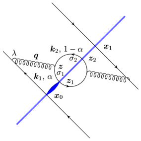
A

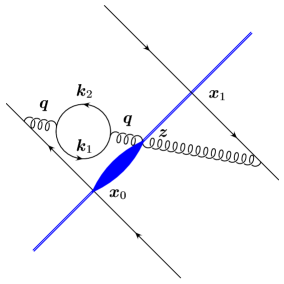
B

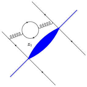
C

Figure 1: Diagrams contributing a factor $N_{f}$ at order $\alpha_{s}^{2}\ln(1/x)$. The line from bottom left to top right indicates the target field crossed by the fast moving constituents of the projectile. Their transverse positions are fixed. The ovals indicate insertions of $N({\bm{x}}_{0},{\bm{z}}_{1},Y)$, $N({\bm{x}}_{0},{\bm{z}},Y)$ and $N({\bm{x}}_{0},{\bm{x}}_{1},Y)$ respectively.

The calculation in [27] followed the rules of the light cone perturbation theory (LCPT) [47, 48]. The diagrams in Fig. 1 should also be understood as LCPT diagrams. The propagators of gluon lines in the graphs A and C in Fig. 1 also include the instantaneous parts.

Here we are interested in the linear evolution: hence only one of the produced dipoles in Figs. 1 A and B continues to have evolution corrections and interacts with the target. In Fig. 1 we show that with an oval denoting the interacting dipole. Indeed either one of the dipoles can interact and later on we will add the contribution with the other dipole interacting with the target.

We start with the contribution to the NLO JIMWLK kernel coming from the diagram A in Fig. 1, which is given by Eq. (17) in [27]:

$${\cal K}_{1}^{\text{NLO}}({\bm{x}}_{0},{\bm{x}}_{1};{\bm{z}}_{1},{\bm{z}}_{2})\,= \,4\,N_{f}\,\int\limits_{0}^{1}d\alpha\,\int\frac{d^{2}k}{(2\pi)^{2}}\frac{d^{2}k^{\prime}}{(2\pi)^{2}}\frac{d^{2}q}{(2\pi)^{2}}\frac{d^{2}q^{\prime}}{(2\pi)^{2}}\ e^{-i{\bm{q}}\cdot({\bm{z}}-{\bm{x}}_{0})+i{\bm{q}}^{\prime}\cdot({\bm{z}}-{\bm{x}}_{1})-i({\bm{k}}-{\bm{k}}^{\prime})\cdot{\bm{z}}_{12}}$$

$$\times\left[\frac{1}{{\bm{q}}^{2}{\bm{q}}^{\prime 2}}\frac{(1-2\alpha)^{2}{\bm{q}}\cdot{\bm{k}}\ {\bm{k}}^{\prime}\cdot{\bm{q}}^{\prime}+{\bm{q}}\cdot{\bm{q}}^{\prime}\ {\bm{k}}\cdot{\bm{k}}^{\prime}-{\bm{q}}\cdot{\bm{k}}^{\prime}\ {\bm{k}}\cdot{\bm{q}}^{\prime}}{\Big{[}{\bm{k}}^{2}+{\bm{q}}^{2}\alpha(1-\alpha)\Big{]}\Big{[}{\bm{k}}^{\prime 2}+{\bm{q}}^{\prime 2}\alpha(1-\alpha)\Big{]}}\right.$$

$$+\frac{2\,\alpha\,(1-\alpha)\,(1-2\alpha)}{\Big{[}{\bm{k}}^{2}+{\bm{q}}^{2}\alpha(1-\alpha)\Big{]}\Big{[}{\bm{k}}^{\prime 2}+{\bm{q}}^{\prime 2}\alpha(1-\alpha)\Big{]}}\,\left(\frac{{\bm{k}}\cdot{\bm{q}}}{{\bm{q}}^{2}}+\frac{{\bm{k}}^{\prime}\cdot{\bm{q}}^{\prime}}{{\bm{q}}^{\prime 2}}\right)$$

$$\left.+\,\frac{4\,\alpha^{2}\,(1-\alpha)^{2}}{\Big{[}{\bm{k}}^{2}+{\bm{q}}^{2}\alpha(1-\alpha)\Big{]}\Big{[}{\bm{k}}^{\prime 2}+{\bm{q}}^{\prime 2}\alpha(1-\alpha)\Big{]}}\right].$$ (24)

At the moment we exclude all the factors of the coupling constant and the color factor, similar to what was done in [27]. The notations used in Eq. (3) are explained in Fig. 1A: the quark and the anti-quark have transverse momenta ${\bm{k}}_{1}$ and ${\bm{k}}_{2}$ and transverse coordinates ${\bm{z}}_{1}$ and ${\bm{z}}_{2}$. The gluon line carries momentum ${\bm{q}}$ in the amplitude. All the transverse momenta in the complex conjugate amplitude are labeled in the same way as momenta in the amplitude only with a prime. The longitudinal fraction of the gluons’ momentum carried by the quark is labeled $\alpha=k_{1+}/(k_{1+}+k_{2+})$. We also note that ${\bm{z}}=\alpha\,{\bm{z}}_{1}+(1-\alpha)\,{\bm{z}}_{2}$, ${\bm{z}}_{12}={\bm{z}}_{1}-{\bm{z}}_{2}$, ${\bm{q}}={\bm{k}}_{1}+{\bm{k}}_{2}$ and ${\bm{k}}={\bm{k}}_{1}(1-\alpha)-{\bm{k}}_{2}\,\alpha$.

Using ${\bm{q}}={\bm{k}}_{1}+{\bm{k}}_{2}$ and ${\bm{k}}={\bm{k}}_{1}(1-\alpha)-{\bm{k}}_{2}\,\alpha$ (and the same for primed ones) we rewrite Eq. (3) as

$${\cal K}_{1}^{\text{NLO}}({\bm{x}}_{0},{\bm{x}}_{1};{\bm{z}}_{1},{\bm{z}}_{2})\,=\,4\,N_{f}\,\int\limits_{0}^{1}d\alpha\,\int\frac{d^{2}k_{1}}{(2\pi)^{2}}\frac{d^{2}k_{2}}{(2\pi)^{2}}\frac{d^{2}k^{\prime}_{1}}{(2\pi)^{2}}\frac{d^{2}k^{\prime}_{2}}{(2\pi)^{2}}$$

$$\times\,e^{-i{\bm{k}}_{1}\cdot({\bm{z}}_{1}-{\bm{x}}_{0})-i{\bm{k}}_{2}\cdot({\bm{z}}_{2}-{\bm{x}}_{0})+i{\bm{k}}^{\prime}_{1}\cdot({\bm{z}}_{1}-{\bm{x}}_{1})+i{\bm{k}}^{\prime}_{2}\cdot({\bm{z}}_{2}-{\bm{x}}_{1})}\,\frac{1}{({\bm{k}}_{1}+{\bm{k}}_{2})^{2}\,({\bm{k}}^{\prime}_{1}+{\bm{k}}^{\prime}_{2})^{2}}$$

$$\times\,\frac{{\bm{k}}_{1}\cdot{\bm{k}}^{\prime}_{1}\,{\bm{k}}_{2}\cdot{\bm{k}}^{\prime}_{2}-{\bm{k}}_{1}\cdot{\bm{k}}^{\prime}_{2}\,{\bm{k}}^{\prime}_{1}\cdot{\bm{k}}_{2}+[{\bm{k}}_{1}\cdot{\bm{k}}_{2}+{\bm{k}}_{1}^{2}\,(1-\alpha)+{\bm{k}}_{2}^{2}\,\alpha]\,[{\bm{k}}^{\prime}_{1}\cdot{\bm{k}}^{\prime}_{2}+{\bm{k}}_{1}^{\prime 2}\,(1-\alpha)+{\bm{k}}_{2}^{\prime 2}\,\alpha]}{[{\bm{k}}_{1}^{2}\,(1-\alpha)+{\bm{k}}_{2}^{2}\,\alpha]\,[{\bm{k}}_{1}^{\prime 2}\,(1-\alpha)+{\bm{k}}_{2}^{\prime 2}\,\alpha]}.$$ (25)

As indicated in Fig. 1A, in the linear regime only one of the dipoles, say the dipole formed by ${\bm{x}}_{0}$ and ${\bm{z}}_{1}$ continues the evolution. Hence there is no dependence on the coordinate ${\bm{z}}_{2}$ in the resulting $N(|{\bm{x}}_{0}-{\bm{z}}_{1}|,Y)$. Therefore we can (and should) integrate ${\bm{z}}_{2}$ out. Adding the result to the other $N_{f}$ corrections leads us to consider the whole contribution as part of the running coupling corrections.

Let us note that this procedure is equivalent to the “UV subtraction” performed by Balitsky in [29] for the nonlinear evolution equation and briefly explain the context. For the nonlinear equations, extraction of the UV-divergent part of the diagram A in Fig. 1, which one must absorb in the running coupling constant, can be done in many ways, depending on which linear combination of ${\bm{z}}_{1}$ and ${\bm{z}}_{2}$ is kept fixed. This choice is referred to in [27], maybe somewhat unfortunately, as the choice of “subtraction point.” Since the notions of “UV subtraction” and “subtraction point” play an important role in the renormalization of QCD, we should attempt to forestall unnecessary confusion by pointing out that the ideas involved here are only peripherally connected to renormalization. The subtractions referred to here correspond to different schemes of separating the running coupling contributions (which must carry the UV divergence of QCD diagrams so that the UV scale $\mu$ will enter the logarithms that induce the running of the coupling) from new physics channels (such as, in this case, the presence of a well separated $\bar{q}q$-pair in the final state), from which the UV divergent running coupling contribution has been subtracted. The only new channel we have considered explicitly, the $\bar{q}q$ channel, then turns out to be completely finite and $\mu$ independent at present accuracy. This separation scheme dependence (and the coordinate space “subtraction points” associated with it) is a freedom that arises independently in addition to the renormalization scheme dependence and the momentum space renormalization scale $\mu$ (with associated subtraction points) appearing in the renormalization procedure of QCD. In the case of non-linear evolution the arbitrariness of the separation scheme results in the differences between [27] and [29]. We emphasize that the total result, in which running coupling contributions and new channels are added together, is not affected by this separation. In contrast to renormalization scheme dependence, which can not be eliminated at any finite order in perturbation theory, this statement about separation scheme independence holds order by order in perturbation theory. In the separation of [27] both the running coupling corrections and the new $q\bar{q}$ channel contribute leading-$N_{f}$ terms to the linear part of the BK equation and the sum of these contributions is obtained by the the above procedure. In the separation of [29], all leading order $N_{f}$–contributions to the linear part of the BK equation are included into the running coupling, while the correspondingly constructed new $q\bar{q}$ channel only contributes a nonlinear term to the BK equation. This establishes the direct correspondence of our present procedure (which is simply aimed at collecting all leading-$N_{f}$ contributions to the linear part of the BK equation) to the subtraction used in [29].

Let us stress again that for the total leading-$N_{f}$ contribution (and that is what we are calculating here) subtraction points are not an issue, they merely affect the separation into what we interpret as a running coupling correction and new production channels. The only remarkable point here is that the leading-$N_{f}$ contributions may all be interpreted as running coupling corrections.

To return to our present task: we are interested in the linear evolution and have to integrate the kernel in Eq. (3) either over ${\bm{z}}_{2}$ or ${\bm{z}}_{1}$ depending on which dipole interacts with the target.

To integrate over ${\bm{z}}_{2}$, which would put ${\bm{k}}^{\prime}_{2}={\bm{k}}_{2}$, we define ${\bm{q}}={\bm{k}}_{1}+{\bm{k}}_{2}$ and ${\bm{q}}^{\prime}={\bm{k}}^{\prime}_{1}+{\bm{k}}^{\prime}_{2}={\bm{k}}^{\prime}_{1}+{\bm{k}}_{2}$, obtaining

$$\int d^{2}z_{2}\,{\cal K}_{1}^{\text{NLO}}({\bm{x}}_{0},{\bm{x}}_{1};{\bm{z}}_{1},{\bm{z}}_{2})\,=\,4\,N_{f}\,\int\limits_{0}^{1}d\alpha\,\int\frac{d^{2}q}{(2\pi)^{2}}\frac{d^{2}q^{\prime}}{(2\pi)^{2}}\frac{d^{2}k}{(2\pi)^{2}}\ e^{-i{\bm{q}}\cdot({\bm{z}}_{1}-{\bm{x}}_{0})+i{\bm{q}}\cdot({\bm{z}}_{1}-{\bm{x}}_{1})}$$

$$\times\,\frac{1}{{\bm{q}}^{2}\,{\bm{q}}^{\prime 2}\,[({\bm{q}}-{\bm{k}})^{2}\,(1-\alpha)+{\bm{k}}^{2}\,\alpha]\,[({\bm{q}}^{\prime}-{\bm{k}})^{2}\,(1-\alpha)+{\bm{k}}^{2}\,\alpha]}$$

$$\times\,\bigg{\{}{\bm{k}}^{2}\,({\bm{q}}-{\bm{k}})\cdot({\bm{q}}^{\prime}-{\bm{k}})-{\bm{k}}\cdot({\bm{q}}-{\bm{k}})\,{\bm{k}}\cdot({\bm{q}}^{\prime}-{\bm{k}})+[{\bm{k}}\cdot({\bm{q}}-{\bm{k}})+({\bm{q}}-{\bm{k}})^{2}\,(1-\alpha)+{\bm{k}}^{2}\,\alpha]$$

$$\times\,[{\bm{k}}\cdot({\bm{q}}^{\prime}-{\bm{k}})+({\bm{q}}^{\prime}-{\bm{k}})^{2}\,(1-\alpha)+{\bm{k}}^{2}\,\alpha]\bigg{\}}$$ (26)

where we dropped the subscript $2$ in ${\bm{k}}_{2}$, i.e., ${\bm{k}}_{2}\rightarrow{\bm{k}}$. Now we have to integrate over ${\bm{k}}$. To do so we first write

$$\int d^{2}z_{2}\,{\cal K}_{1}^{\text{NLO}}({\bm{x}}_{0},{\bm{x}}_{1};{\bm{z}}_{1},{\bm{z}}_{2})\,=\,4\,N_{f}\,\int\limits_{0}^{1}d\alpha\,\int\frac{d^{2}q}{(2\pi)^{2}}\frac{d^{2}q^{\prime}}{(2\pi)^{2}}\frac{d^{d}k}{(2\pi)^{d}}\ e^{-i{\bm{q}}\cdot({\bm{z}}_{1}-{\bm{x}}_{0})+i{\bm{q}}\cdot({\bm{z}}_{1}-{\bm{x}}_{1})}$$

$$\times\,\frac{1}{{\bm{q}}^{2}\,{\bm{q}}^{\prime 2}}\,\Bigg{\{}\frac{{\bm{k}}^{2}\,({\bm{q}}-{\bm{k}})\cdot({\bm{q}}^{\prime}-{\bm{k}})}{[({\bm{q}}-{\bm{k}})^{2}\,(1-\alpha)+{\bm{k}}^{2}\,\alpha]\,[({\bm{q}}^{\prime}-{\bm{k}})^{2}\,(1-\alpha)+{\bm{k}}^{2}\,\alpha]}$$

$$+\frac{{\bm{k}}\cdot({\bm{q}}-{\bm{k}})}{({\bm{q}}-{\bm{k}})^{2}\,(1-\alpha)+{\bm{k}}^{2}\,\alpha}+\frac{{\bm{k}}\cdot({\bm{q}}^{\prime}-{\bm{k}})}{({\bm{q}}^{\prime}-{\bm{k}})^{2}\,(1-\alpha)+{\bm{k}}^{2}\,\alpha}+1\Bigg{\}},$$ (27)

where, in anticipation of dimensional regularization we have inserted the dimension $d$ of the ${\bm{k}}$-integral explicitly. The details of ${\bm{k}}$-integration in Eq. (3) are given in Appendix B. The result yields

$$\int d^{2}z_{2}\,{\cal K}_{1}^{\text{NLO}}({\bm{x}}_{0},{\bm{x}}_{1};{\bm{z}}_{1},{\bm{z}}_{2})\,=\,\frac{N_{f}}{3\,\pi}\,\int\frac{d^{2}q}{(2\pi)^{2}}\frac{d^{2}q^{\prime}}{(2\pi)^{2}}\,\ e^{-i{\bm{q}}\cdot({\bm{z}}_{1}-{\bm{x}}_{0})+i{\bm{q}}\cdot({\bm{z}}_{1}-{\bm{x}}_{1})}$$

$$\times\,\frac{1}{{\bm{q}}^{2}\,{\bm{q}}^{\prime 2}}\Bigg{\{}({\bm{q}}-{\bm{q}}^{\prime})^{2}\,\ln\frac{({\bm{q}}-{\bm{q}}^{\prime})^{2}\,e^{-5/3}}{\mu_{\overline{\text{MS}}}^{2}}-{\bm{q}}^{2}\,\ln\frac{{\bm{q}}^{2}\,e^{-5/3}}{\mu_{\overline{\text{MS}}}^{2}}-{\bm{q}}^{\prime 2}\,\ln\frac{{\bm{q}}^{\prime 2}\,e^{-5/3}}{\mu_{\overline{\text{MS}}}^{2}}\Bigg{\}}.$$ (28)

Note that due to the symmetry property

$${\cal K}_{1}^{\text{NLO}}({\bm{x}}_{0},{\bm{x}}_{1};{\bm{z}}_{1},{\bm{z}}_{2})\,=\,{\cal K}_{1}^{\text{NLO}}({\bm{x}}_{0},{\bm{x}}_{1};{\bm{z}}_{2},{\bm{z}}_{1})$$ (29)

the contribution to the NLO BFKL kernel of Fig. 1A with the dipole formed by ${\bm{z}}_{2}$ and ${\bm{x}}_{1}$ interacting is equal to the right hand side of Eq. (3) with ${\bm{z}}_{1}\rightarrow{\bm{z}}_{2}$.

To construct the full leading-$N_{f}$ NLO BFKL kernel one has to add to Eq. (3) the contribution to the NLO BFKL kernel ${\cal K}_{2}^{\text{NLO}}$ of the diagram B from Fig. 1. Using Eq. (28) in [27] along with its mirror reflection with respect to the line denoting the interaction with the target we obtain

$$\int d^{2}z_{2}\,{\cal K}_{1}^{\text{NLO}}({\bm{x}}_{0},{\bm{x}}_{1};{\bm{z}}_{1},{\bm{z}}_{2})+{\cal K}_{2}^{\text{NLO}}({\bm{x}}_{0},{\bm{x}}_{1};{\bm{z}}_{1})\,=\,\frac{N_{f}}{3\,\pi}\,\int\frac{d^{2}q}{(2\pi)^{2}}\frac{d^{2}q^{\prime}}{(2\pi)^{2}}\,\ e^{-i{\bm{q}}\cdot({\bm{z}}_{1}-{\bm{x}}_{0})+i{\bm{q}}\cdot({\bm{z}}_{1}-{\bm{x}}_{1})}$$

$$\times\,\frac{1}{{\bm{q}}^{2}\,{\bm{q}}^{\prime 2}}\Bigg{\{}({\bm{q}}-{\bm{q}}^{\prime})^{2}\,\ln\frac{({\bm{q}}-{\bm{q}}^{\prime})^{2}\,e^{-5/3}}{\mu_{\overline{\text{MS}}}^{2}}-{\bm{q}}^{2}\,\ln\frac{{\bm{q}}^{2}\,e^{-5/3}}{\mu_{\overline{\text{MS}}}^{2}}-{\bm{q}}^{\prime 2}\,\ln\frac{{\bm{q}}^{\prime 2}\,e^{-5/3}}{\mu_{\overline{\text{MS}}}^{2}}$$

$$+2\,{\bm{q}}\cdot{\bm{q}}^{\prime}\,\ln\frac{{\bm{q}}^{2}\,e^{-5/3}}{\mu_{\overline{\text{MS}}}^{2}}+\,2\,{\bm{q}}\cdot{\bm{q}}^{\prime}\,\ln\frac{{\bm{q}}^{\prime 2}\,e^{-5/3}}{\mu_{\overline{\text{MS}}}^{2}}\Bigg{\}}.$$ (30)

The above expression can be simplified to give

$$\int d^{2}z_{2}\,{\cal K}_{1}^{\text{NLO}}({\bm{x}}_{0},{\bm{x}}_{1};{\bm{z}}_{1},{\bm{z}}_{2})+{\cal K}_{2}^{\text{NLO}}({\bm{x}}_{0},{\bm{x}}_{1};{\bm{z}}_{1})\,=\,\frac{N_{f}}{3\,\pi}\,\int\frac{d^{2}q}{(2\pi)^{2}}\frac{d^{2}q^{\prime}}{(2\pi)^{2}}\,\ e^{-i{\bm{q}}\cdot({\bm{z}}_{1}-{\bm{x}}_{0})+i{\bm{q}}\cdot({\bm{z}}_{1}-{\bm{x}}_{1})}$$

$$\times\,\frac{1}{{\bm{q}}^{2}\,{\bm{q}}^{\prime 2}}\Bigg{\{}{\bm{q}}^{2}\,\ln\frac{({\bm{q}}-{\bm{q}}^{\prime})^{2}}{{\bm{q}}^{2}}+{\bm{q}}^{\prime 2}\,\ln\frac{({\bm{q}}-{\bm{q}}^{\prime})^{2}}{{\bm{q}}^{\prime 2}}+\,2\,{\bm{q}}\cdot{\bm{q}}^{\prime}\,\ln\frac{{\bm{q}}^{2}\,{\bm{q}}^{\prime 2}}{({\bm{q}}-{\bm{q}}^{\prime})^{2}\,\mu^{2}}\Bigg{\}},$$ (31)

where we have also defined $\mu^{2}=\mu_{\overline{M}S}^{2}\,e^{5/3}$.

We do not need to calculate explicitly the diagram in Fig. 1 C due to the real-virtual cancellations which lead to the identity

$$\int d^{2}z_{2}\,{\cal K}_{1}^{\text{NLO}}({\bm{x}}_{0},{\bm{x}}_{1};{\bm{z}}_{1},{\bm{z}}_{2})+{\cal K}_{2}^{\text{NLO}}({\bm{x}}_{0},{\bm{x}}_{1};{\bm{z}}_{1})+{\cal K}_{3}^{\text{NLO}}({\bm{x}}_{0},{\bm{x}}_{1};{\bm{z}}_{1})\,=\,0.$$ (32)

Here

$$\int d^{2}z_{1}\,{\cal K}_{3}^{\text{NLO}}({\bm{x}}_{0},{\bm{x}}_{1};{\bm{z}}_{1})$$

is the contribution of Fig. 1 C represented as the integral over the transverse coordinate of the (anti-)quark.

The full leading-$N_{f}$ NLO dipole kernel is defined via

$$K^{\text{NLO}}_{f}({\bm{x}}_{0},{\bm{x}}_{1};{\bm{z}}_{1})\,=\,\frac{N_{c}}{2}\,\sum_{m,n=0}^{1}\,(-1)^{m+n}\left\{\int d^{2}z_{2}\,{\cal K}_{1}^{\text{NLO}}({\bm{x}}_{m},{\bm{x}}_{n};{\bm{z}}_{1},{\bm{z}}_{2})+{\cal K}_{2}^{\text{NLO}}({\bm{x}}_{m},{\bm{x}}_{n};{\bm{z}}_{1})\right\}$$ (33)

where we have included the color factor $N_{c}/2$ in the large-$N_{c}$ approximation and have summed over all possible emissions of the gluon in Fig. 1 off the quark and the anti-quark lines in the original dipole.

Including the contributions of either one of the dipoles in Figs. 1 A and B interacting with the target we derive that the additive NLO contribution to the right hand side of Eq. (1) is given by

$$\alpha_{\mu}^{2}\,\int d^{2}x_{2}\,K^{\text{NLO}}_{f}({\bm{x}}_{0},{\bm{x}}_{1};{\bm{x}}_{2})\,\left[N({\bm{x}}_{0},{\bm{x}}_{2},Y)+N({\bm{x}}_{2},{\bm{x}}_{1},Y)-N({\bm{x}}_{0},{\bm{x}}_{1},Y)\right],$$ (34)

where $\alpha_{\mu}$ is the bare coupling constant. In the discussion of LO BFKL the running of the coupling was negligible: hence we did not distinguish the bare coupling from the physical coupling and labeled them $\alpha_{s}$. At the NLO level running coupling corrections become important and we will start distinguishing between the two.

Combining Eqs. (3) and (33) yields an additive NLO modification of the LO dipole kernel from Eq. (8) of the form

$$K_{{\bm{q}},{\bm{q}}^{\prime}}\,\to\,\alpha_{\mu}\frac{{\bm{q}}\cdot{\bm{q}}^{\prime}+\alpha_{\mu}\frac{N_{f}}{3\pi}\left({\bm{q}}^{2}\,\ln\frac{({\bm{q}}-{\bm{q}}^{\prime})^{2}}{{\bm{q}}^{2}}+{\bm{q}}^{\prime 2}\,\ln\frac{({\bm{q}}-{\bm{q}}^{\prime})^{2}}{{\bm{q}}^{\prime 2}}+\,2\,{\bm{q}}\cdot{\bm{q}}^{\prime}\,\ln\frac{{\bm{q}}^{2}\,{\bm{q}}^{\prime 2}}{({\bm{q}}-{\bm{q}}^{\prime})^{2}\,\mu^{2}}\right)}{{\bm{q}}^{2}\,{\bm{q}}^{\prime 2}}.$$ (35)

Since our manipulations leading to the evolution equation (10) did not make use of any special properties of the kernel, we only need to form linear combinations according to (12) and (11) to find the evolution equation for the unintegrated gluon distribution function defined in Eq. (15)

$$\alpha_{s}(k^{2})\,\frac{\partial\phi(k,Y)}{\partial Y}\,=\,\frac{\alpha_{\mu}\,N_{c}}{\pi^{2}}\,\int d^{2}q\left[\frac{\alpha_{s}(q^{2})}{({\bm{k}}-{\bm{q}})^{2}}\,\phi(q,Y)-\alpha_{s}(k^{2})\,\frac{{\bm{k}}\cdot({\bm{k}}-{\bm{q}})}{{\bm{q}}^{2}\,({\bm{k}}-{\bm{q}})^{2}}\,\phi(k,Y)\right]+\frac{\alpha_{\mu}^{2}\,N_{c}\,N_{f}}{12\,\pi^{3}}$$

$$\times\,\int d^{2}q\,\left[\frac{2\,\alpha_{s}(q^{2})}{({\bm{k}}-{\bm{q}})^{2}}\,\ln\left(\frac{{\bm{k}}^{2}\,({\bm{k}}-{\bm{q}})^{2}}{{\bm{q}}^{2}\,\mu^{2}}\right)\,\phi(q,Y)-\frac{\alpha_{s}(k^{2})\,{\bm{k}}^{2}}{{\bm{q}}^{2}\,({\bm{k}}-{\bm{q}})^{2}}\,\ln\left(\frac{{\bm{q}}^{2}\,({\bm{k}}-{\bm{q}})^{2}}{{\bm{k}}^{2}\,\mu^{2}}\right)\,\phi(k,Y)\right].$$ (36)

Here we could not neglect the running of the coupling and kept the factors of the physical coupling $\alpha_{s}$ introduced in the definition of the unintegrated gluon distribution in Eq. (15). However, as we are interested in the NLO correction only, we should divide both sides of Eq. (3) by $\alpha_{s}(k^{2})$ and expand the kernel on the right hand side of the resulting equation up to the second order in $\alpha_{\mu}$ using

$$\frac{\alpha_{s}(q^{2})}{\alpha_{s}(k^{2})}\,\approx\,1+\alpha_{\mu}\,\beta_{2}\,\ln\frac{k^{2}}{q^{2}}\,\rightarrow\,1-\frac{\alpha_{\mu}\,N_{f}}{6\,\pi}\,\ln\frac{k^{2}}{q^{2}}.$$ (37)

Here

$$\beta_{2}\,=\,\frac{11\,N_{c}-2\,N_{f}}{12\,\pi}$$ (38)

and we replaced $\beta_{2}\rightarrow-N_{f}/6\pi$ since we are interested in leading-$N_{f}$ contribution only.

With the expansion of Eq. (37) we finally obtain

$$\frac{\partial\phi(k,Y)}{\partial Y}\,=\,\frac{\alpha_{\mu}\,N_{c}}{2\,\pi^{2}}\,\int d^{2}q\left[\frac{2}{({\bm{k}}-{\bm{q}})^{2}}\,\phi(q,Y)-\frac{{\bm{k}}^{2}}{{\bm{q}}^{2}\,({\bm{k}}-{\bm{q}})^{2}}\,\phi(k,Y)\right]+\frac{\alpha_{\mu}^{2}\,N_{c}\,N_{f}}{12\,\pi^{3}}$$

$$\times\,\int d^{2}q\,\left[\frac{2}{({\bm{k}}-{\bm{q}})^{2}}\,\ln\left(\frac{({\bm{k}}-{\bm{q}})^{2}}{\mu^{2}}\right)\,\phi(q,Y)-\frac{{\bm{k}}^{2}}{{\bm{q}}^{2}\,({\bm{k}}-{\bm{q}})^{2}}\,\ln\left(\frac{{\bm{q}}^{2}\,({\bm{k}}-{\bm{q}})^{2}}{{\bm{k}}^{2}\,\mu^{2}}\right)\,\phi(k,Y)\right].$$ (39)

Eq. (3) is the BFKL equation with the leading-$N_{f}$ NLO correction calculated in the large-$N_{c}$ approximation.

4 Resummation of bubble diagrams: triumvirate
couplings for forward BFKL

The leading-$N_{f}$ NLO BFKL kernel in Eq. (3) is remarkably simple, appearing to be more compact than the similar kernel obtained using conventional perturbation theory in [30, 34]. To understand the origin of this simplicity let us point out that, using the techniques developed in [27] one can resum the $\alpha_{\mu}\,N_{f}$ corrections to all orders, which correspond diagrammatically to inserting an infinite chain of quark loops on the gluon line emitted in one step of small-$x$ evolution in the $s$-channel approach. Replacing $N_{f}\rightarrow-6\,\pi\,\beta_{2}$ and absorbing all the corrections into the running coupling constant we obtain the JIMWLK kernel with resummed running coupling corrections

$$\alpha_{\mu}\,{\cal K}_{\text{rc}}({\bm{x}}_{0},{\bm{x}}_{1};{\bm{z}})\,=\,4\,\int\frac{d^{2}q}{(2\pi)^{2}}\frac{d^{2}q^{\prime}}{(2\pi)^{2}}\ e^{-i{\bm{q}}\cdot({\bm{z}}-{\bm{x}}_{0})+i{\bm{q}}^{\prime}\cdot({\bm{z}}-{\bm{x}}_{1})}\,\frac{{\bm{q}}\cdot{\bm{q}}^{\prime}}{{\bm{q}}^{2}\,{\bm{q}}^{\prime 2}}\,\frac{\alpha_{s}\left({\bm{q}}^{2}\,e^{-5/3}\right)\,\alpha_{s}\left({\bm{q}}^{\prime 2}\,e^{-5/3}\right)}{\alpha_{s}\left(Q^{2}\,e^{-5/3}\right)}\ ,$$ (40)

where

$$\ln\frac{Q^{2}\,e^{-5/3}}{\mu_{\overline{{\text{MS}}}}^{2}}\,\equiv\,\frac{1}{2\,{\bm{q}}\cdot{\bm{q}}^{\prime}}\,\Bigg{\{}{\bm{q}}^{2}\,\ln\frac{{\bm{q}}^{2}\,e^{-5/3}}{\mu_{\overline{\text{MS}}}^{2}}+{\bm{q}}^{\prime 2}\,\ln\frac{{\bm{q}}^{\prime 2}\,e^{-5/3}}{\mu_{\overline{\text{MS}}}^{2}}-({\bm{q}}-{\bm{q}}^{\prime})^{2}\,\ln\frac{({\bm{q}}-{\bm{q}}^{\prime})^{2}\,e^{-5/3}}{\mu_{\overline{\text{MS}}}^{2}}\Bigg{\}}.$$ (41)

This expression leads to a remarkably simple form for the building blocks of the forward kernels for the angular averaged case: We find

$$K_{{\bm{q}},{\bm{q}}^{\prime}}\to K^{\text{NLO}}_{{\bm{q}},{\bm{q}}^{\prime}}=\frac{1}{2}\left\{\frac{\alpha_{s}({\bm{q}}^{2}\,e^{-5/3})}{{\bm{q}}^{2}}+\frac{\alpha_{s}({\bm{q}}^{\prime 2}\,e^{-5/3})}{{\bm{q}}^{\prime 2}}-\frac{\alpha_{s}({\bm{q}}^{2}\,e^{-5/3})\alpha_{s}({\bm{q}}^{\prime 2}\,e^{-5/3})}{\alpha_{s}(({\bm{q}}-{\bm{q}}^{\prime})^{2}\,e^{-5/3})}\frac{({\bm{q}}-{\bm{q}}^{\prime})^{2}}{{\bm{q}}^{2}{\bm{q}}^{\prime 2}}\right\},$$ (42a)

$$L_{{\bm{q}},{\bm{q}}^{\prime}}\to L^{\text{NLO}}_{{\bm{q}},{\bm{q}}^{\prime}}=\frac{1}{2}\left\{\frac{\alpha_{s}({\bm{q}}^{2}\,e^{-5/3})}{{\bm{q}}^{2}}-\frac{\alpha_{s}({\bm{q}}^{\prime 2}\,e^{-5/3})}{{\bm{q}}^{\prime 2}}+\frac{\alpha_{s}({\bm{q}}^{2}\,e^{-5/3})\alpha_{s}({\bm{q}}^{\prime 2}\,e^{-5/3})}{\alpha_{s}(({\bm{q}}-{\bm{q}}^{\prime})^{2}\,e^{-5/3})}\frac{({\bm{q}}-{\bm{q}}^{\prime})^{2}}{{\bm{q}}^{2}{\bm{q}}^{\prime 2}}\right\}.$$ (42b)

Since the kernel in the real part is an explicitly symmetric combination of $L$’s, one can immediately read off (dropping the NLO superscript for brevity)

$$L_{\bm{q}-{\bm{k}},-{\bm{k}}}+ L_{-{\bm{k}},\bm{q}-{\bm{k}}}+L_{{\bm{k}},\bm{k}-{\bm{q}}}+L_{{\bm{k}}-{\bm{q}},{\bm{k}}}=2\ \frac{\alpha_{s}({\bm{k}}^{2}\,e^{-5/3})\ \alpha_{s}(({\bm{q}}-{\bm{k}})^{2}\,e^{-5/3})}{\alpha_{s}({\bm{q}}^{2}\,e^{-5/3})}\frac{{\bm{q}}^{2}}{{\bm{k}}^{2}({\bm{q}}-{\bm{k}})^{2}}\ .$$ (43)

For the virtual contribution one notes that the antisymmetric parts of both terms integrate to zero (by a shift in ${\bm{q}}$). We reverse the sign of ${\bm{q}}$ in the remainder of the second term and are left with

$$\int\!d^{2}q\Big{(}L_{{\bm{q}},\bm{q}-{\bm{k}}}+L_{{\bm{q}},\bm{q}+{\bm{k}}}\Big{)}=\int\!d^{2}q\ \frac{\alpha_{s}({\bm{q}}^{2}\,e^{-5/3})\alpha_{s}(({\bm{q}}-{\bm{k}})^{2}\,e^{-5/3})}{\alpha_{s}({\bm{k}}^{2}\,e^{-5/3})}\frac{{\bm{k}}^{2}}{{\bm{q}}^{2}({\bm{q}}-{\bm{k}})^{2}}.$$ (44)

Collecting all the contributions one obtains an equation for $\tilde{N}(k,Y)$:

$$\frac{\partial\tilde{N}(k,Y)}{\partial Y}\,=\,\frac{N_{c}}{2\pi^{2}}\int d^{2}q\ \Bigg{\{} 2\ \frac{\alpha_{s}({\bm{k}}^{2}\,e^{-5/3})\alpha_{s}(({\bm{q}}-{\bm{k}})^{2}\,e^{-5/3})}{\alpha_{s}({\bm{q}}^{2}\,e^{-5/3})}\frac{{\bm{q}}^{2}}{{\bm{k}}^{2}({\bm{q}}-{\bm{k}})^{2}}\tilde{N}(q,Y)$$

$$-\frac{\alpha_{s}({\bm{q}}^{2}\,e^{-5/3})\alpha_{s}(({\bm{q}}-{\bm{k}})^{2}\,e^{-5/3})}{\alpha_{s}({\bm{k}}^{2}\,e^{-5/3})}\frac{{\bm{k}}^{2}}{{\bm{q}}^{2}({\bm{q}}-{\bm{k}})^{2}}\tilde{N}(k,Y)\Bigg{\}}.$$ (45)

Using Eq. (15) in Eq. (4) yields the following evolution equation for the unintegrated gluon distribution including running coupling corrections to all orders

$$\frac{\partial\phi(k,Y)}{\partial Y}\,=\,\frac{N_{c}}{2\,\pi^{2}}\,\int d^{2}q\,\Bigg{\{} \frac{2}{({\bm{k}}-{\bm{q}})^{2}}\,\alpha_{s}\left(({\bm{k}}-{\bm{q}})^{2}\,e^{-5/3}\right)\,\phi(q,Y)$$

$$-\frac{{\bm{k}}^{2}}{{\bm{q}}^{2}\,({\bm{k}}-{\bm{q}})^{2}}\,\frac{\alpha_{s}\left({\bm{q}}^{2}\,e^{-5/3}\right)\,\alpha_{s}\left(({\bm{k}}-{\bm{q}})^{2}\,e^{-5/3}\right)}{\alpha_{s}\left({\bm{k}}^{2}\,e^{-5/3}\right)}\,\phi(k,Y)\Bigg{\}}.$$ (46)

Expanding Eq. (4) in powers of $\alpha_{\mu}$ to order $\alpha_{\mu}^{2}$ would yield Eq. (3). Hence, from the standpoint of linear evolution, the simplicity of the leading-$N_{f}$ NLO BFKL kernel obtained here is due to the fact that this kernel consists only of running coupling corrections.

Eq. (4) should be compared with the evolution equation for the unintegrated gluon distribution derived in [40] (c.f. Eqs. (22) and (23) there). At first sight Eq. (4) appears to disagree with these expressions. However, defining a new function

$${\tilde{\phi}}(k,Y)\,=\,\frac{\phi(k,Y)}{\alpha_{s}\left({\bm{k}}^{2}\,e^{-5/3}\right)}$$ (47)

we recast Eq. (4) into

$$\frac{\partial{\tilde{\phi}}(k,Y)}{\partial Y}\,=\,\frac{N_{c}}{2\,\pi^{2}}\,\int d^{2}q \ \frac{\alpha_{s}\left({\bm{q}}^{2}\,e^{-5/3}\right)\,\alpha_{s}\left(({\bm{k}}-{\bm{q}})^{2}\,e^{-5/3}\right)}{\alpha_{s}\left({\bm{k}}^{2}\,e^{-5/3}\right)}$$

$$\times\,\Bigg{\{}\frac{2}{({\bm{k}}-{\bm{q}})^{2}}\,{\tilde{\phi}}(q,Y)-\frac{{\bm{k}}^{2}}{{\bm{q}}^{2}\,({\bm{k}}-{\bm{q}})^{2}}\,{\tilde{\phi}}(k,Y)\Bigg{\}}.$$ (48)

Eq. (4) is in agreement with Eqs. (22) and (23) of [40]. Eq. (47) links the evolving quantity to the unintegrated gluon distribution.

Eq. (4) was originally obtained in [40] by calculating running coupling corrections to the virtual contributions in the non-forward case. This result was then generalized to include running coupling corrections also to the real contribution by postulating the validity of the bootstrap equation beyond leading order [40, 39]. To understand if this postulate can be justified from our calculations, we need to explore also the non-forward case.

5 Generalization to non-forward BFKL: triumvirate
couplings and bootstrap ideas

Now that the general techniques are already familiar we relax our restrictions to forward BFKL and angular averaged results. This will lead us to abandon our initial assumption of impact parameter independence. Practically this amounts to use a Fourier–representation of the lowest order expansions of $N({\bm{x}}_{0},{\bm{x}}_{1},Y)$ shown in Eq. (4) using two independent momenta. We define

$$G_{{\bm{x}}_{i},{\bm{x}}_{j}}=\parbox{85.35826pt}{\includegraphics[width=85.35826pt]{Gdef-coord-cut}};\hskip 28.45274ptG_{{\bm{k}},{\bm{k}}^{\prime}}=\parbox{85.35826pt}{\includegraphics[width=85.35826pt]{Gdef-mom-cut}}\ ,$$ (49)

which are related to each other by the double Fourier–transform

$$G_{{\bm{x}}_{i},{\bm{x}}_{j}}= \int\!\frac{d^{2}k}{(2\pi)^{2}}\frac{d^{2}k^{\prime}}{(2\pi)^{2}}e^{i{\bm{k}}\cdot{\bm{x}}_{i}+i{\bm{k}}^{\prime}\cdot{\bm{x}}_{j}}G_{{\bm{k}},{\bm{k}}^{\prime}}=\int\!\frac{d^{2}k}{(2\pi)^{2}}\frac{d^{2}l}{(2\pi)^{2}}e^{i{\bm{k}}\cdot({\bm{x}}_{i}-{\bm{x}}_{j})+i{\bm{l}}\cdot\frac{{\bm{x}}_{i}+{\bm{x}}_{j}}{2}}G_{{\bm{k}}+\frac{{\bm{l}}}{2},{\bm{k}}-\frac{{\bm{l}}}{2}}\ .$$ (50)

After the second equality sign we have changed integration variables to conjugates of the relative and absolute positions in a form most suitable to our calculations below. With this definition Eq. (3) is replaced by

$$N({\bm{x}}_{i},{\bm{x}}_{j},Y)= \frac{1}{2}\int\!\frac{d^{2}k}{(2\pi)^{2}}\frac{d^{2}l}{(2\pi)^{2}}\left(e^{i{\bm{l}}\cdot{\bm{x}}_{i}}+e^{i{\bm{l}}{\bm{x}}_{j}}-e^{i{\bm{k}}\cdot{\bm{x}}_{ij}+i{\bm{l}}\cdot\frac{{\bm{x}}_{i}+{\bm{x}}_{j}}{2}}-e^{-i{\bm{k}}\cdot{\bm{x}}_{ij}+i{\bm{l}}\cdot\frac{{\bm{x}}_{i}+{\bm{x}}_{j}}{2}}\right)G_{{\bm{k}}+\frac{{\bm{l}}}{2},{\bm{k}}-\frac{{\bm{l}}}{2}}(Y)$$

$$+\text{higher orders}$$ (51)

in a term by term correspondence with Eq. (4). Despite this change compared to the forward case, one can still proceed to extract the (non-forward) BFKL equation using a technique that completely parallels the steps used in Sec. 2. The only price to pay is additional algebraic effort. In this spirit, we insert our expressions for $N({\bm{x}}_{i},{\bm{x}}_{j},Y)$ and a generic kernel of the form (8) into the linearized BK equation (1) as before. We will later use the resummed expressions shown in (42) to obtain explicit results.

In our calculation, we first perform the ${\bm{x}}_{2}$–integral to eliminate the ${\bm{q}}^{\prime}$ dependence and again use shifts and sign reflections in ${\bm{q}}$ to cast the result in the form

$$\frac{\partial}{\partial Y} \int\!\frac{d^{2}k}{(2\pi)^{2}}\frac{d^{2}l}{(2\pi)^{2}}\left(e^{i{\bm{l}}\cdot{\bm{x}}_{0}}+e^{i{\bm{l}}{\bm{x}}_{1}}-e^{i{\bm{k}}\cdot{\bm{x}}_{01}+i{\bm{l}}\cdot\frac{{\bm{x}}_{0}+{\bm{x}}_{1}}{2}}-e^{-i{\bm{k}}\cdot{\bm{x}}_{01}+i{\bm{l}}\cdot\frac{{\bm{x}}_{0}+{\bm{x}}_{1}}{2}}\right)G_{{\bm{k}}+\frac{{\bm{l}}}{2},{\bm{k}}-\frac{{\bm{l}}}{2}}(Y)$$

$$= \int\!\frac{d^{2}k}{(2\pi)^{2}}\frac{d^{2}l}{(2\pi)^{2}}\frac{N_{c}}{2\pi^{2}}\int d^{2}q\ \ \left\{\left(e^{i{\bm{l}}\cdot{\bm{x}}_{0}}+e^{i{\bm{l}}{\bm{x}}_{1}}-e^{i{\bm{q}}\cdot{\bm{x}}_{01}+i{\bm{l}}\cdot\frac{{\bm{x}}_{0}+{\bm{x}}_{1}}{2}}-e^{-i{\bm{q}}\cdot{\bm{x}}_{01}+i{\bm{l}}\cdot\frac{{\bm{x}}_{0}+{\bm{x}}_{1}}{2}}\right)K_{\text{real}}({\bm{q}},{\bm{k}},{\bm{l}})\right.$$

$$\left.\hskip 28.45274pt-\left(e^{i{\bm{l}}\cdot{\bm{x}}_{0}}+e^{i{\bm{l}}{\bm{x}}_{1}}-e^{i{\bm{k}}\cdot{\bm{x}}_{01}+i{\bm{l}}\cdot\frac{{\bm{x}}_{0}+{\bm{x}}_{1}}{2}}-e^{-i{\bm{k}}\cdot{\bm{x}}_{01}+i{\bm{l}}\cdot\frac{{\bm{x}}_{0}+{\bm{x}}_{1}}{2}}\right)K_{\text{virt}}({\bm{k}},{\bm{q}},{\bm{l}})\right\}G_{{\bm{k}}+\frac{{\bm{l}}}{2},{\bm{k}}-\frac{{\bm{l}}}{2}}(Y).$$ (52)

The kernels can again be expressed in terms of $L_{{\bm{q}},{\bm{q}}^{\prime}}$ as before in the forward case. We find

$$K_{\text{real}}({\bm{k}},{\bm{q}},{\bm{l}}) =L_{{\bm{k}}-\frac{\bm{l}}{2},-{\bm{q}}+{\bm{k}}}-L_{{\bm{k}}-\frac{\bm{l}}{2},{\bm{k}}+\frac{\bm{l}}{2}}-L_{{\bm{q}}-{\bm{k}},-{\bm{k}}+\frac{\bm{l}}{2}}+L_{-{\bm{k}}-\frac{\bm{l}}{2},{\bm{q}}-{\bm{k}}}-L_{-{\bm{k}}-\frac{\bm{l}}{2},-{\bm{k}}+\frac{\bm{l}}{2}}+L_{-{\bm{q}}+{\bm{k}},{\bm{k}}+\frac{\bm{l}}{2}},$$ (53a)

$$K_{\text{virt}}({\bm{k}},{\bm{q}},{\bm{l}}) =L_{{\bm{q}},-{\bm{k}}+\frac{\bm{l}}{2}+{\bm{q}}}+L_{{\bm{q}},{\bm{k}}+\frac{\bm{l}}{2}+{\bm{q}}}.$$ (53b)

In these expressions we have already anticipated the swap of ${\bm{k}}$ and ${\bm{q}}$ in the real term to facilitate the last step, in which we read off the equation for $G_{{\bm{k}}+\frac{{\bm{l}}}{2},{\bm{k}}-\frac{{\bm{l}}}{2}}(Y)$ by equating the integrands:

$$\frac{\partial\,G_{{\bm{k}}+\frac{{\bm{l}}}{2},{\bm{k}}-\frac{{\bm{l}}}{2}}(Y)}{\partial Y}= \frac{N_{c}}{2\pi^{2}}\int d^{2}q\ \Big{\{}K_{\text{real}}({\bm{k}},{\bm{q}},{\bm{l}})G_{{\bm{q}}+\frac{{\bm{l}}}{2},{\bm{q}}-\frac{{\bm{l}}}{2}}(Y)-K_{\text{virt}}({\bm{k}},{\bm{q}},{\bm{l}})G_{{\bm{k}}+\frac{{\bm{l}}}{2},{\bm{k}}-\frac{{\bm{l}}}{2}}(Y)\Big{\}}$$ (54)

Last, we insert the explicit expressions of Eq. (42) into (53) and repeat the arguments of the forward case to again cancel the antisymmetric parts. Anticipating a comparison with Levin and Braun [40, 39] we introduce the notation

$$\eta\left({\bm{k}}^{2}\right):=\frac{{\bm{k}}^{2}}{\alpha_{s}\left({\bm{k}}^{2}\,e^{-5/3}\right)}$$ (55)

and change notation by shifting both ${\bm{k}}$ and ${\bm{q}}$ by $-{\bm{l}}/2$. Note that [40, 39] do not specify the renormalization scheme and hence do not keep track of the factors $e^{-5/3}$ we take care to include here.

With these conventions, the final equation reads

$$\frac{\partial\,G_{{\bm{k}},{\bm{k}}-{\bm{l}}}(Y)}{\partial Y}= \frac{N_{c}}{2\pi^{2}}\int d^{2}q\ K_{\text{real}}({\bm{k}},{\bm{q}},{\bm{l}})\ G_{{\bm{q}},{\bm{q}}-{\bm{l}}}(Y)-\left[\beta\left(\left({\bm{k}}-{\bm{l}}\right)^{2}\right)+\beta\left({\bm{k}}^{2}\right)\right]G_{{\bm{k}},{\bm{k}}-{\bm{l}}}(Y)$$ (56)

where the real kernel takes the explicit form

$$K_{\text{real}}({\bm{k}},{\bm{q}},{\bm{l}})=\frac{\eta\left(\left({\bm{q}}-\bm{l}\right)^{2}\right)}{\eta\left(\left({\bm{k}}-\bm{l}\right)^{2}\right)\eta\left((\left({\bm{k}}-\bm{q}\right)^{2}\right)}+\frac{\eta\left({\bm{q}}^{2}\right)}{\eta\left({\bm{k}}^{2}\right)\eta\left(\left({\bm{k}}-\bm{q}\right)^{2}\right)}-\frac{\eta\left({\bm{l}}^{2}\right)}{\eta\left({\bm{k}}^{2}\right)\eta\left(\left({\bm{k}}-\bm{l}\right)^{2}\right)}$$ (57)

and $\beta\left({\bm{k}}^{2}\right)$ denotes the gluon trajectory defined as

$$\beta\left({\bm{k}}^{2}\right)=\frac{N_{c}}{2\pi^{2}}\int d^{2}q\ \frac{1}{2}\frac{\eta\left({\bm{k}}^{2}\right)}{\eta\left({\bm{q}}^{2}\right)\eta\left(\left({\bm{k}}-\bm{q}\right)^{2}\right)}\ .$$ (58)

We note that all individual contributions are composed of triumvirate structures. In the forward limit, this reduces to what we found earlier in (4) with $\tilde{N}(k,Y)\approx G_{\bm{k},\bm{k}}(Y)$.

We now wish to compare to [40, 39], without loosing the connection with the bootstrap condition used in their argument. This prevents us from taking the forward limit (which we have already shown at the end of Sec. 4). Instead, we identify the quantity used in [40, 39] by amputating the external, coupling–resummed gluon legs from the dipole scattering amplitude $G_{{\bm{k}},{\bm{k}}^{\prime}}(Y)$: we separate out a factor $\frac{\alpha_{s}\left({\bm{k}}^{2}\right)}{{\bm{k}}^{2}}\frac{\alpha_{s}\left(\left({\bm{k}}^{\prime}\right)^{2}\right)}{{\bm{k}}^{\prime 2}}$ according to

$$G_{{\bm{k}},{\bm{k}}^{\prime}}(Y)=\parbox{85.35826pt}{\includegraphics[width=85.35826pt]{Gdef-mom-cut}}=\frac{\alpha_{s}\left({\bm{k}}^{2}\,e^{-5/3}\right)}{{\bm{k}}^{2}}\frac{\alpha_{s}\left({\bm{k}}^{\prime 2}\,e^{-5/3}\right)}{{\bm{k}}^{\prime 2}}\ \varphi_{{\bm{k}},{\bm{k}}^{\prime}}(Y)\ .$$ (59)

Generically, such modifications leave the gluon Regge trajectories unaffected and rescale only the real kernel. Here, the real kernel is modified to

$$\tilde{K}_{\text{real}}({\bm{k}},{\bm{q}},{\bm{l}})= K_{\text{real}}({\bm{q}},{\bm{k}},{\bm{l}})\ \frac{\eta\left({\bm{k}}^{2}\right)\eta\left(\left({\bm{k}}-{\bm{l}}\right)^{2}\right)}{\eta\left({\bm{q}}^{2}\right)\eta\left(\left({\bm{q}}-{\bm{l}}\right)^{2}\right)}$$

$$= \frac{\eta\left(\left({\bm{k}}-\bm{l}\right)^{2}\right)}{\eta\left(\left({\bm{q}}-\bm{l}\right)^{2}\right)\eta\left((\left({\bm{k}}-\bm{q}\right)^{2}\right)}+\frac{\eta\left({\bm{k}}^{2}\right)}{\eta\left({\bm{q}}^{2}\right)\eta\left(\left({\bm{k}}-\bm{q}\right)^{2}\right)}-\frac{\eta\left({\bm{l}}^{2}\right)}{\eta\left({\bm{q}}^{2}\right)\eta\left(\left({\bm{k}}-\bm{l}\right)^{2}\right)}\ .$$ (60)

This turns Eq. (56) into

$$\frac{\partial\varphi_{{\bm{k}},{\bm{k}}-{\bm{l}}}(Y)}{\partial Y}= \frac{N_{c}}{2\pi^{2}}\int d^{2}q\ \tilde{K}_{\text{real}}({\bm{k}},{\bm{q}},{\bm{l}})\ \varphi_{{\bm{q}},{\bm{q}}-{\bm{l}}}(Y)-\left[\beta\left(\left({\bm{k}}-{\bm{l}}\right)^{2}\right)+\beta\left({\bm{k}}^{2}\right)\right]\varphi_{{\bm{k}},{\bm{k}}-{\bm{l}}}(Y)\ .$$ (61)

The structures in this equation correspond directly to (16) of [40] or (4) of [39], which, as already mentioned, were based on calculating the running coupling corrections to the virtual contributions and postulating a bootstrap condition to extend the result to include corrections for the real contributions.

Our calculation now provides a derivation of this statement in the $s$-channel light cone perturbation theory formalism, previously used to derive the JIMWLK and BK equations, and gives a firm interpretation of the objects involved.

6 Leading-$N_{f}$ contribution to the NLO BFKL pomeron intercept

To find the leading-$N_{f}$ contribution to the NLO BFKL intercept (in the large-$N_{c}$ limit) we have to act on $\phi(k,Y)\sim k^{2\,\lambda}$ with the NLO part of the kernel in Eq. (3). Employing Eq. (19) again and using the same notation as in Sect. 2.2 we write

$$\int d^{2}q\,K^{\text{NLO}}_{f}({\bm{k}},{\bm{q}})\,q^{2\,\lambda}\,\equiv$$

$$\equiv\,\int d^{2}q\,\left[\frac{2}{({\bm{k}}-{\bm{q}})^{2}}\,\ln\left(\frac{({\bm{k}}-{\bm{q}})^{2}}{\mu^{2}}\right)\,q^{2\,\lambda}-\frac{{\bm{k}}^{2}}{{\bm{q}}^{2}\,({\bm{k}}-{\bm{q}})^{2}}\,\ln\left(\frac{{\bm{q}}^{2}\,({\bm{k}}-{\bm{q}})^{2}}{{\bm{k}}^{2}\,\mu^{2}}\right)\,k^{2\,\lambda}\right]$$

$$=\,2\pi\,\int\limits_{0}^{\infty}db\,b\,J_{0}(b\,k)\,\int\limits_{\Lambda}^{\infty}dq\,q\,J_{0}(b\,q)\,\int\limits_{\Lambda}^{\infty}dl\,l^{-1}\,J_{0}(b\,l)\times\,\left[2\,\ln\left(\frac{l^{2}}{\mu^{2}}\right)\,q^{2\,\lambda}-\frac{k^{2}}{q^{2}}\,\ln\left(\frac{q^{2}\,l^{2}}{k^{2}\,\mu^{2}}\right)\,k^{2\,\lambda}\right]$$ (62)

Integrating over $q$ and $l$ with the help of formulae in Appendix A yields

$$\int d^{2}q\,K^{\text{NLO}}_{f}({\bm{k}},{\bm{q}})\,q^{2\,\lambda}\,=$$

$$=2\pi\,\int\limits_{0}^{\infty}db\,b\,J_{0}(b\,k)\,\left(\psi(1)-\ln\frac{b\,\Lambda}{2}\right)\,\Bigg{\{}2^{2\lambda+2}\,b^{-2\lambda-2}\,\frac{\Gamma\left(1+\lambda\right)}{\Gamma\left(-\lambda\right)}\,\left[\psi(1)-\ln\frac{b\,\mu^{2}}{2\,\Lambda}\right]$$

$$-2\,k^{2\,\lambda+2}\,\left(\psi(1)-\ln\frac{b\,\Lambda}{2}\right)\,\left(\psi(1)-\ln\frac{b\,k\,\mu}{2\,\Lambda}\right)\Bigg{\}}.$$ (63)

Finally, using formulae in Appendix A to integrate Eq. (6) over $b$ we obtain

$$\int d^{2}q\,K^{\text{NLO}}_{f}({\bm{k}},{\bm{q}})\,q^{2\,\lambda}\,=\,2\pi\,k^{2\,\lambda}\,\left\{\frac{1}{2}\,\chi^{2}(-\lambda)+\chi(-\lambda)\,\ln\frac{k^{2}}{\mu^{2}}+\frac{1}{2}\,\psi^{\prime}(-\lambda)-\frac{1}{2}\,\psi^{\prime}(1+\lambda)\right\}.$$ (64)

Including the prefactor of $\frac{\alpha_{\mu}^{2}\,N_{c}\,N_{f}}{12\,\pi^{3}}$ which we have been omitting above, combining (64) with the leading order contribution to the intercept (22) and remembering that $\mu^{2}=\mu_{\overline{M}S}^{2}\,e^{5/3}$ yields

$$\frac{\alpha_{\mu}\,N_{c}}{\pi}\,\int d^{2}q\,K^{\text{LO}}({\bm{k}},{\bm{q}})\,\left(\frac{q}{k}\right)^{2\,\lambda}+\frac{\alpha_{\mu}^{2}\,N_{c}\,N_{f}}{12\,\pi^{3}}\,\int d^{2}q\,K^{\text{NLO}}_{f}({\bm{k}},{\bm{q}})\,\left(\frac{q}{k}\right)^{2\,\lambda}\,=$$

$$=\frac{\alpha_{\mu}N_{c}}{\pi}\left\{\chi(-\lambda)\left[1-\alpha_{\mu}\,\beta_{2}\,\ln\frac{k^{2}}{\mu_{\overline{\text{MS}}}^{2}}\right]-\frac{\alpha_{\mu}N_{f}}{12\,\pi}\left[-\chi^{2}(-\lambda)-\psi^{\prime}(-\lambda)+\psi^{\prime}(1+\lambda)+\frac{10}{3}\,\chi(-\lambda)\right]\right\}$$ (65)

where we have replaced $N_{f}\rightarrow-6\pi\beta_{2}$ in front of the logarithm to underline the fact that this separation of terms has often been interpreted a separation of running coupling and conformal contributions.

From our earlier considerations in Sec. 3, we now know that such a separation is artificial. In fact the discussion there and in Sec. 4 as well as Sec. 5 allow us to take the extreme position and assign all contributions listed here to running coupling effects. To facilitate comparison with [34, 30], we still introduce the notation $\Delta(\lambda)$ for the last term in Eq. (6) by

$$\frac{\alpha_{\mu}\,N_{c}}{\pi}\,\int d^{2}q\,K^{\text{LO}}({\bm{k}},{\bm{q}})\,\left(\frac{q}{k}\right)^{2\,\lambda}+ \frac{\alpha_{\mu}^{2}\,N_{c}\,N_{f}}{12\,\pi^{3}}\,\int d^{2}q\,K^{\text{NLO}}_{f}({\bm{k}},{\bm{q}})\,\left(\frac{q}{k}\right)^{2\,\lambda}\,=$$

$$=\,\frac{\alpha_{\mu}\,N_{c}}{\pi}\,\Bigg{\{}\chi(-\lambda)\,\bigg{[}1-\alpha_{\mu}\,\beta_{2}\, \ln\frac{k^{2}}{\mu_{\overline{\text{MS}}}^{2}}\bigg{]}-\frac{\alpha_{\mu}\,N_{f}}{12\,\pi}\,\Delta(\lambda)\Bigg{\}}\ .$$ (66)

From Eq. (6) we have

$$\Delta(\lambda)\,=\,-\chi^{2}(-\lambda)-\psi^{\prime}(-\lambda)+\psi^{\prime}(1+\lambda)+\frac{10}{3}\,\chi(-\lambda).$$ (67)

To compare our result with the result of the NLO calculation of Fadin and Lipatov [30] and of Camici and Ciafaloni [34] we note that in [30, 34] instead of the power $\lambda$ the authors used the power $\gamma-1$, such that $\lambda=\gamma-1$. We thus first rewrite Eq. (67) in terms of $\gamma$

$$\Delta(\gamma)\,=\,-\chi^{2}(\gamma)-\psi^{\prime}(1-\gamma)+\psi^{\prime}(\gamma)+\frac{10}{3}\,\chi(\gamma).$$ (68)

The intercept of Eq. (68) exactly agrees with the result of Fadin and Lipatov (see Eqs. (14) and (12) in [30]) and with the result of Camici and Ciafaloni (see Eq. (4.6) in [34])! We have thus provided an independent cross-check of those earlier results [34, 30].

It is important to note that the agreement between the intercepts of [34, 30] and the one in Eq. (68) depends crucially on the fact that both intercepts were calculated for the same observable — the unintegrated gluon distribution. We also stress that the factor of $\alpha_{s}(k^{2})$ in the definition of the unintegrated gluon distribution in Eq. (15) plays an important role in obtaining the correct intercept.

7 Comparison with the NLO intercept for the evolution of dipole amplitude calculated in [29]

Another leading-$N_{f}$ NLO BFKL intercept we should compare with is due to a transverse coordinate space calculation performed by Balitsky [29]. The result of [29], expressed in terms of the same power $\gamma$ as defined in [34, 30] reads (see Eq. (44) in [29])

$$\Delta_{\text{B}}(\gamma)\,=\,\chi^{2}(\gamma)+\psi^{\prime}(1-\gamma)-\psi^{\prime}(\gamma)-\frac{4}{1-\gamma}\,\chi(\gamma)+\frac{10}{3}\,\chi(\gamma).$$ (69)

We will demonstrate below that this expression can be translated into the corresponding (uniquely defined) contribution in the results of [34, 30] and our earlier result Eq. (68), by taking into account that (i) $\Delta_{\text{B}}(\gamma)$ was obtained using both kernels and eigenfunctions in transverse coordinate space and that (ii) $\Delta_{\text{B}}(\gamma)$ is the intercept for a different observable — the forward scattering amplitude for a dipole on the target, while $\Delta(\gamma)$ was calculated for the unintegrated gluon distribution in momentum space.

We will, therefore, show that after a Fourier transform relating $\phi(k,Y)$ to $N(x_{01},Y)$, our intercept from Eq. (68) is translates into the intercept $\Delta_{\text{B}}(\gamma)$ from Eq. (69) obtained in [29]. Combining Eq. (2) with Eq. (3) we write

$$N(x_{01},Y)\,=\,\frac{2\,\pi}{N_{c}}\,\int d^{2}k\,(1-e^{i{\bm{k}}\cdot{\bm{x}}_{01}})\,\frac{\alpha_{s}(k^{2})\,\phi(k,Y)}{k^{2}}.$$ (70)

Therefore, if we put $\alpha_{s}(k^{2})\,\phi(k,Y)\,=\,k^{2\,\lambda}$ then we would obtain

$$N(x_{01},Y)\,=\,-\frac{(2\,\pi)^{2}}{N_{c}}\,2^{2\,\lambda-1}\,x_{01}^{-2\,\lambda}\,\frac{\Gamma(\lambda)}{\Gamma(1-\lambda)}.$$ (71)

Using Eq. (3) and the steps which led to it we write

$$\alpha_{\mu}^{2}\,\int d^{2}x_{2}\,K^{\text{NLO}}_{f}({\bm{x}}_{0},{\bm{x}}_{1};{\bm{x}}_{2})\,\left[N({\bm{x}}_{0},{\bm{x}}_{2},Y)+N({\bm{x}}_{2},{\bm{x}}_{1},Y)-N({\bm{x}}_{0},{\bm{x}}_{1},Y)\right]$$

$$\,=\,\frac{2\,\pi}{N_{c}}\,\int\frac{d^{2}k}{{\bm{k}}^{2}}\,(1-e^{i{\bm{k}}\cdot{\bm{x}}_{01}})\,\frac{\alpha_{\mu}^{2}\,N_{c}\,N_{f}}{12\,\pi^{3}}\,\int d^{2}q\,\left[K^{\text{NLO}}_{f}({\bm{k}},{\bm{q}})+\frac{2}{({\bm{k}}-{\bm{q}})^{2}}\,\ln\frac{{\bm{k}}^{2}}{{\bm{q}}^{2}}\right]\,\alpha_{s}(q^{2})\,\phi(q,Y).$$ (72)

Therefore, for $N(x_{01},Y)=x_{01}^{-2\,\lambda}$,

$$\alpha_{\mu}^{2}\,K_{f}^{\text{NLO}}\,\otimes\,x_{01}^{-2\,\lambda}\,=\,-\frac{2^{-2\,\lambda+1}}{2\,\pi}\,\frac{\Gamma(1-\lambda)}{\Gamma(\lambda)}\int\frac{d^{2}k}{{\bm{k}}^{2}}\,(1-e^{i{\bm{k}}\cdot{\bm{x}}_{01}})$$

$$\times\,\frac{\alpha_{\mu}^{2}\,N_{c}\,N_{f}}{12\,\pi^{3}}\,\int d^{2}q\,\left[K^{\text{NLO}}_{f}({\bm{k}},{\bm{q}})+\frac{2}{({\bm{k}}-{\bm{q}})^{2}}\,\ln\frac{{\bm{k}}^{2}}{{\bm{q}}^{2}}\right]\,q^{2\,\lambda},$$ (73)

where we have abbreviated the action of the NLO kernel on the left hand side of Eq. (7). To perform the part of $q$-integral involving $K^{\text{NLO}}_{f}({\bm{k}},{\bm{q}})$ we will employ Eq. (64). The rest of the $q$-integral is

$$\int d^{2}q\,\frac{2}{({\bm{k}}-{\bm{q}})^{2}}\,\ln\frac{{\bm{k}}^{2}}{{\bm{q}}^{2}}\,q^{2\,\lambda}\,=\,2\,\pi\,\left[\psi^{\prime}(1+\lambda)-\psi^{\prime}(-\lambda)\right]\,k^{2\,\lambda},$$ (74)

which can be derived using Eq. (19) and the formulae in Appendix A. Combining this with Eq. (64) yields

$$\alpha_{\mu}^{2}\,K_{f}^{\text{NLO}}\,\otimes\,x_{01}^{-2\,\lambda}\,=\,-2^{-2\,\lambda+1}\,\frac{\Gamma(1-\lambda)}{\Gamma(\lambda)}\int\frac{d^{2}k}{{\bm{k}}^{2}}\,(1-e^{i{\bm{k}}\cdot{\bm{x}}_{01}})$$

$$\times\,\frac{\alpha_{\mu}^{2}\,N_{c}\,N_{f}}{12\,\pi^{3}}\,k^{2\,\lambda}\,\left\{\frac{1}{2}\,\chi^{2}(-\lambda)+\chi(-\lambda)\,\ln\frac{k^{2}}{\mu^{2}}-\frac{1}{2}\,\psi^{\prime}(-\lambda)+\frac{1}{2}\,\psi^{\prime}(1+\lambda)\right\}.$$ (75)

Performing the integration over ${\bm{k}}$ we obtain

$$\alpha_{\mu}^{2}\,K_{f}^{\text{NLO}}\,\otimes\,x_{01}^{-2\,\lambda}\,=\,\frac{\alpha_{\mu}^{2}\,N_{c}\,N_{f}}{6\,\pi^{2}}\,\Bigg{\{}\frac{1}{2}\,\chi^{2}(-\lambda)+\chi(-\lambda)\,\left[\ln\frac{4\,e^{-2\,\gamma}}{x_{01}^{2}\,\mu^{2}}-\chi(-\lambda)-\frac{2}{\lambda}\right]$$

$$-\,\frac{1}{2}\,\psi^{\prime}(-\lambda)+\frac{1}{2}\,\psi^{\prime}(1+\lambda)\Bigg{\}}\,x_{01}^{-2\,\lambda},$$ (76)

where $\gamma=-\psi(1)$ is the Euler’s constant. Since the LO BFKL kernel acting on a power in transverse coordinate space gives the usual BFKL eigenvalue

$$\alpha_{\mu}\,K^{\text{LO}}\,\otimes\,x_{01}^{-2\,\lambda}\,=\,\frac{\alpha_{\mu}\,N_{c}}{\pi}\,\chi(-\lambda)\,x_{01}^{-2\,\lambda}$$ (77)

we write

$$\left[\alpha_{\mu}\,K^{\text{LO}}+\alpha_{\mu}^{2}\,K_{f}^{\text{NLO}}\right]\otimes\,x_{01}^{-2\,\lambda}\,=\,\frac{\alpha_{\mu}\,N_{c}}{\pi}\,\Bigg{\{}\chi(-\lambda)\,\left[1-\alpha_{\mu}\,\beta_{2}\,\ln\frac{4\,e^{-2\,\gamma}}{x_{01}^{2}\,\mu^{2}_{\overline{\text{MS}}}}\right]-\frac{\alpha_{\mu}\,N_{f}}{12\,\pi}\,\Delta_{B}(\lambda)\Bigg{\}}\,x_{01}^{-2\,\lambda}$$ (78)

with

$$\Delta_{B}(\lambda)\,=\,\chi^{2}(-\lambda)+\frac{4}{\lambda}\,\chi(-\lambda)+\psi^{\prime}(-\lambda)-\psi^{\prime}(1+\lambda)+\frac{10}{3}\,\chi(-\lambda).$$ (79)

Here one might worry that this value of $\Delta_{B}(\lambda)$ depends on our choice of the constant under the logarithm in Eq. (78). However this choice is not arbitrary and is consistent with the constant obtained under the logarithm of the coordinate space running coupling corrections resummed to all orders in [27]. (In [27] we would also have a factor of $e^{-5/3}$ under the running coupling logarithm. Here, following the convention of [34, 30, 29] we have chosen to place this contribution separately: it leads to the $\frac{10}{3}\,\chi(-\lambda)$ term in Eq. (79).)

Replacing $\lambda=\gamma-1$ reduces Eq. (79) to Eq. (69)! We have thus shown that our intercept (68) and the intercept in Eq. (69) found in [29] are consistent with each other. The difference between them is due to the fact that they are calculated for two different observables.

8 Conclusions

In this paper we have studied the implications for the linear BFKL evolution equation of including running coupling corrections into the non-linear JIMWLK and BK evolution equations performed in [27]. In particular we have derived the BFKL equation including running coupling corrections to all orders and calculated the leading-$N_{f}$ NLO BFKL pomeron intercept. Until now the form of the BFKL equation with all orders resummed running coupling corrections was not known. What existed was a conjecture by Braun and by Levin [39, 40] based on an interesting assumption that bootstrap equations hold even with running coupling corrections included. We have shown that this conjecture is in fact accurate, though for a slightly different observable than suggested originally. Our results were derived using the $s$-channel language of light cone perturbation theory [47, 48]. Up to now the NLO BFKL intercept had only been calculated either by using the standard Feynman perturbation theory in [34, 30] and or by employing the background field method [29]. Our calculation provides an independent check of the intercept found in [34, 30] and connects it to the one obtained in [29].

Our paper has two main results. First of all, we have obtained the BFKL equation for the unintegrated gluon distribution including running coupling corrections resummed to all orders. The equation is given by (4). After a redefinition of the unintegrated gluon distribution shown in Eq. (47), Eq. (4) leads to Eq. (4), which was conjectured by Braun and by Levin in [39, 40] by postulating the bootstrap condition in the running coupling case. We have thus shown that the conjecture of [39, 40] for the BFKL equation with the running coupling corrections is correct, though for a slightly non-traditional definition of the unintegrated gluon distribution (47). We have clarified that this result is based on a complete absorption of all $\alpha_{s}\,N_{f}$ corrections into the running of the coupling in the BFKL equation (as in Eq. (4)). This is one of many possible constructions as explained in Sec. 3, all others would separate off explicit $N_{f}$–contributions that are not interpreted as running coupling contributions. The result Eq. (4) is formulated in the form of a “triumvirate” of the couplings [27].

Our second result is an independent check of the leading-$N_{f}$ contribution to the NLO BFKL intercept (expanded to strictly NLO, without any resummations), which we performed in Sect. 6. Our intercept, obtained for the evolution of the unintegrated gluon distribution function, is given by Eq. (68) and completely agrees with the results of Camici and Ciafaloni [34] and of Fadin and Lipatov [30]. The NLO intercept appears to strongly depend on the physical observable: we demonstrate that by calculating the leading-$N_{f}$ NLO BFKL intercept for the dipole scattering amplitude, starting from that of the unintegrated gluon distribution. Our result is given in Eq. (79) and agrees with the result of Balitsky [29]. The difference in the expressions (67) and (79) is fully explained by the fact that the two intercepts refer to different observables.

Appendix A Useful formulae

Here we list some useful mathematical formulae. The main formula we need above is

$$\int\limits_{0}^{\infty}dl\,l^{2\lambda+1}\,J_{0}(b\,l)\,=\,2^{2\lambda+1}\,b^{-2\lambda-2}\,\frac{\Gamma\left(1+\lambda\right)}{\Gamma\left(-\lambda\right)}.$$ (A1)

Using Eq. (A1) one can derive the following useful results (here $b>0$):

$$\int\limits_{\Lambda}^{\infty}dl\,l^{-1}\,J_{0}(b\,l)\,=\,\psi(1)-\ln\frac{b\,\Lambda}{2},$$ (A2)

$$\int\limits_{\Lambda}^{\infty}dl\,l^{-1}\,J_{0}(b\,l)\,\ln l^{2}=\,\left(\psi(1)-\ln\frac{b\,\Lambda}{2}\right)\,\left(\psi(1)-\ln\frac{b}{2\,\Lambda}\right),$$ (A3)

$$\int\limits_{0}^{\infty}dl\,l\,J_{0}(b\,l)\,=\,0,$$ (A4)

$$\int\limits_{0}^{\infty}dl\,l\,J_{0}(b\,l)\,\ln l\,=\,-\frac{1}{b^{2}},$$ (A5)

$$\int\limits_{0}^{\infty}dl\,l\,J_{0}(b\,l)\,\ln^{2}l\,=\,\frac{2}{b^{2}}\,\left[\ln\left(\frac{b}{2}\right)-\psi(1)\right],$$ (A6)

$$\int\limits_{0}^{\infty}dl\,l\,J_{0}(b\,l)\,\ln^{3}l\,=\,-\frac{3}{b^{2}}\,\left[\ln\left(\frac{b}{2}\right)-\psi(1)\right]^{2}.$$ (A7)

Appendix B Evaluating Eq. (3)

Our goal here is to perform the $\bm{k}$-integration in Eq. (3). We begin with the first term in the curly brackets in Eq. (3). Performing the $\alpha$-integral first we obtain

$$4\,N_{f}\,\int\frac{d^{2}q}{(2\pi)^{2}}\frac{d^{2}q^{\prime}}{(2\pi)^{2}}\frac{d^{d}k}{(2\pi)^{d}}\ e^{-i{\bm{q}}\cdot({\bm{z}}_{1}-{\bm{x}}_{0})+i{\bm{q}}\cdot({\bm{z}}_{1}-{\bm{x}}_{1})}\,\frac{1}{{\bm{q}}^{2}\,{\bm{q}}^{\prime 2}}\,\frac{({\bm{q}}-{\bm{k}})\cdot({\bm{q}}^{\prime}-{\bm{k}})}{({\bm{q}}-{\bm{k}})^{2}-({\bm{q}}^{\prime}-{\bm{k}})^{2}}\,\ln\frac{({\bm{q}}-{\bm{k}})^{2}}{({\bm{q}}^{\prime}-{\bm{k}})^{2}}.$$ (B1)

Eq. (B1) can be rewritten as

$$4\,N_{f}\,\int\frac{d^{2}q}{(2\pi)^{2}}\frac{d^{2}q^{\prime}}{(2\pi)^{2}}\frac{d^{d}k}{(2\pi)^{d}}\ e^{-i{\bm{q}}\cdot({\bm{z}}_{1}-{\bm{x}}_{0})+i{\bm{q}}\cdot({\bm{z}}_{1}-{\bm{x}}_{1})}\,\frac{1}{{\bm{q}}^{2}\,{\bm{q}}^{\prime 2}}\,({\bm{q}}-{\bm{k}})\cdot({\bm{q}}^{\prime}-{\bm{k}})$$

$$\times\,\int\limits_{0}^{1}\,d\beta\,\frac{1}{({\bm{q}}-{\bm{k}})^{2}\,(1-\beta)+({\bm{q}}^{\prime}-{\bm{k}})^{2}\,\beta}.$$ (B2)

Defining a new integration variable ${\tilde{\bm{k}}}={\bm{k}}-(1-\beta)\,{\bm{q}}-\beta\,{\bm{q}}^{\prime}$ we get

$$4\,N_{f}\,\int\frac{d^{2}q}{(2\pi)^{2}}\frac{d^{2}q^{\prime}}{(2\pi)^{2}}\ e^{-i{\bm{q}}\cdot({\bm{z}}_{1}-{\bm{x}}_{0})+i{\bm{q}}\cdot({\bm{z}}_{1}-{\bm{x}}_{1})}\,\frac{1}{{\bm{q}}^{2}\,{\bm{q}}^{\prime 2}}\,\int\limits_{0}^{1}\,d\beta\,\int\frac{d^{d}{\tilde{k}}}{(2\pi)^{d}}\,\frac{{\tilde{\bm{k}}}^{2}-\beta\,(1-\beta)\,({\bm{q}}-{\bm{q}}^{\prime})^{2}}{{\tilde{\bm{k}}}^{2}+\beta\,(1-\beta)\,({\bm{q}}-{\bm{q}}^{\prime})^{2}},$$ (B3)

where we dropped the terms linear in ${\tilde{\bm{k}}}$ in the numerator as they vanish after angular integration. Performing the ${\tilde{\bm{k}}}$-integral yields

$$-8\,N_{f}\,\int\frac{d^{2}q}{(2\pi)^{2}}\frac{d^{2}q^{\prime}}{(2\pi)^{2}}\ e^{-i{\bm{q}}\cdot({\bm{z}}_{1}-{\bm{x}}_{0})+i{\bm{q}}\cdot({\bm{z}}_{1}-{\bm{x}}_{1})}\,\frac{1}{{\bm{q}}^{2}\,{\bm{q}}^{\prime 2}}\,\int\limits_{0}^{1}\,d\beta\ \frac{\Gamma\left(1-\frac{d}{2}\right)}{(4\,\pi)^{d/2}}\,\left[\beta\,(1-\beta)\,({\bm{q}}-{\bm{q}}^{\prime})^{2}\right]^{d/2}.$$ (B4)

Inserting $d=2-\epsilon$, expanding the expression in powers of $\epsilon$, replacing $1/\epsilon$ with $\ln\mu_{MS}$ and integrating over $\beta$ yields

$$\frac{N_{f}}{3\,\pi}\,\int\frac{d^{2}q}{(2\pi)^{2}}\frac{d^{2}q^{\prime}}{(2\pi)^{2}}\ e^{-i{\bm{q}}\cdot({\bm{z}}_{1}-{\bm{x}}_{0})+i{\bm{q}}\cdot({\bm{z}}_{1}-{\bm{x}}_{1})}\,\frac{1}{{\bm{q}}^{2}\,{\bm{q}}^{\prime 2}}\,({\bm{q}}-{\bm{q}}^{\prime})^{2}\,\ln\frac{({\bm{q}}-{\bm{q}}^{\prime})^{2}\,e^{-5/3}}{\mu_{\overline{\text{MS}}}^{2}}$$ (B5)

where $\mu_{\overline{\text{MS}}}^{2}=\mu_{MS}^{2}\,4\pi\,e^{-\gamma}$. Eq. (B5) gives us the first term in the curly brackets of Eq. (3).

The last term in the curly brackets of Eq. (3) gives us zero after performing a dimensionally regularized $\bm{k}$-integral. We are left only with the second and the third terms in the curly brackets of Eq. (3), which are analogous to each other. Here we will show how to do the $\bm{k}$-integration in the second term only: the integral in the third term can be easily done in the the same way.

Defining ${\tilde{\bm{k}}}={\bm{k}}-(1-\alpha)\,{\bm{q}}$ the second term in the curly brackets of Eq. (3) can be written as

$$-4\,N_{f}\,\int\frac{d^{2}q}{(2\pi)^{2}}\frac{d^{2}q^{\prime}}{(2\pi)^{2}}\ e^{-i{\bm{q}}\cdot({\bm{z}}_{1}-{\bm{x}}_{0})+i{\bm{q}}\cdot({\bm{z}}_{1}-{\bm{x}}_{1})}\,\frac{1}{{\bm{q}}^{2}\,{\bm{q}}^{\prime 2}}\,\int\limits_{0}^{1}\,d\alpha\,\int\frac{d^{d}{\tilde{k}}}{(2\pi)^{d}}\,\frac{{\tilde{\bm{k}}}^{2}-\alpha\,(1-\alpha)\,{\bm{q}}^{2}}{{\tilde{\bm{k}}}^{2}+\alpha\,(1-\alpha)\,{\bm{q}}^{2}},$$ (B6)

which, repeating the above steps which led from Eq. (B3) to Eq. (B5), can be recast into

$$-\frac{N_{f}}{3\,\pi}\,\int\frac{d^{2}q}{(2\pi)^{2}}\frac{d^{2}q^{\prime}}{(2\pi)^{2}}\ e^{-i{\bm{q}}\cdot({\bm{z}}_{1}-{\bm{x}}_{0})+i{\bm{q}}\cdot({\bm{z}}_{1}-{\bm{x}}_{1})}\,\frac{1}{{\bm{q}}^{\prime 2}}\,\ln\frac{{\bm{q}}^{2}\,e^{-5/3}}{\mu_{\overline{\text{MS}}}^{2}}.$$ (B7)

This is exactly the second term in the curly brackets of Eq. (3). The third term is done by analogy with the second one.

References

- [1] E. A. Kuraev, L. N. Lipatov, and V. S. Fadin, The Pomeranchuk singularity in non-Abelian gauge theories, Sov. Phys. JETP 45 (1977) 199–204.
- [2] Y. Y. Balitsky and L. N. Lipatov Sov. J. Nucl. Phys. 28 (1978) 822.
- [3] I. Balitsky, Operator expansion for high-energy scattering, Nucl. Phys. B463 (1996) 99–160, [hep-ph/9509348].
- [4] I. Balitsky, Operator expansion for diffractive high-energy scattering, hep-ph/9706411.
- [5] I. Balitsky, Factorization and high-energy effective action, Phys. Rev. D60 (1999) 014020, [hep-ph/9812311].
- [6] Y. V. Kovchegov, Small-x structure function of a nucleus including multiple pomeron exchanges, Phys. Rev. D60 (1999) 034008, [hep-ph/9901281].
- [7] Y. V. Kovchegov, Unitarization of the BFKL pomeron on a nucleus, Phys. Rev. D61 (2000) 074018, [hep-ph/9905214].
- [8] J. Jalilian-Marian, A. Kovner, A. Leonidov, and H. Weigert, The BFKL equation from the Wilson renormalization group, Nucl. Phys. B504 (1997) 415–431, [hep-ph/9701284].
- [9] J. Jalilian-Marian, A. Kovner, A. Leonidov, and H. Weigert, The Wilson renormalization group for low x physics: Towards the high density regime, Phys. Rev. D59 (1999) 014014, [hep-ph/9706377].
- [10] J. Jalilian-Marian, A. Kovner, and H. Weigert, The Wilson renormalization group for low x physics: Gluon evolution at finite parton density, Phys. Rev. D59 (1999) 014015, [hep-ph/9709432].
- [11] J. Jalilian-Marian, A. Kovner, A. Leonidov, and H. Weigert, Unitarization of gluon distribution in the doubly logarithmic regime at high density, Phys. Rev. D59 (1999) 034007, [hep-ph/9807462].
- [12] A. Kovner, J. G. Milhano, and H. Weigert, Relating different approaches to nonlinear QCD evolution at finite gluon density, Phys. Rev. D62 (2000) 114005, [hep-ph/0004014].
- [13] H. Weigert, Unitarity at small Bjorken x, Nucl. Phys. A703 (2002) 823–860, [hep-ph/0004044].
- [14] E. Iancu, A. Leonidov, and L. D. McLerran, Nonlinear gluon evolution in the color glass condensate. I, Nucl. Phys. A692 (2001) 583–645, [hep-ph/0011241].
- [15] E. Ferreiro, E. Iancu, A. Leonidov, and L. McLerran, Nonlinear gluon evolution in the color glass condensate. II, Nucl. Phys. A703 (2002) 489–538, [hep-ph/0109115].
- [16] L. V. Gribov, E. M. Levin, and M. G. Ryskin, Singlet structure function at small x: Unitarization of gluon ladders, Nucl. Phys. B188 (1981) 555–576.
- [17] A. H. Mueller and J.-w. Qiu, Gluon recombination and shadowing at small values of x, Nucl. Phys. B268 (1986) 427.
- [18] L. D. McLerran and R. Venugopalan, Green’s functions in the color field of a large nucleus, Phys. Rev. D50 (1994) 2225–2233, [hep-ph/9402335].
- [19] L. D. McLerran and R. Venugopalan, Gluon distribution functions for very large nuclei at small transverse momentum, Phys. Rev. D49 (1994) 3352–3355, [hep-ph/9311205].
- [20] L. D. McLerran and R. Venugopalan, Computing quark and gluon distribution functions for very large nuclei, Phys. Rev. D49 (1994) 2233–2241, [hep-ph/9309289].
- [21] Y. V. Kovchegov, Non-Abelian Weizsäcker-Williams field and a two- dimensional effective color charge density for a very large nucleus, Phys. Rev. D54 (1996) 5463–5469, [hep-ph/9605446].
- [22] Y. V. Kovchegov, Quantum structure of the non-Abelian Weizsäcker-Williams field for a very large nucleus, Phys. Rev. D55 (1997) 5445–5455, [hep-ph/9701229].
- [23] J. Jalilian-Marian, A. Kovner, L. D. McLerran, and H. Weigert, The intrinsic glue distribution at very small x, Phys. Rev. D55 (1997) 5414–5428, [hep-ph/9606337].
- [24] E. Iancu and R. Venugopalan, The color glass condensate and high energy scattering in QCD, hep-ph/0303204.
- [25] H. Weigert, Evolution at small : The Color Glass Condensate, Prog. Part. Nucl. Phys. 55 (2005) 461–565, [hep-ph/0501087].
- [26] J. Jalilian-Marian and Y. V. Kovchegov, Saturation physics and deuteron gold collisions at RHIC, Prog. Part. Nucl. Phys. 56 (2006) 104–231, [hep-ph/0505052].
- [27] Y. Kovchegov and H. Weigert, Triumvirate of Running Couplings in Small- Evolution, accepted for publication in Nucl. Phys. A (2006) [hep-ph/0609090].
- [28] E. Gardi, K. Rummukainen, J. Kuokkanen, and H. Weigert, Running coupling at small : A dispersive approach, hep-ph/0609087.
- [29] I. I. Balitsky, Quark Contribution to the Small- Evolution of Color Dipole, hep-ph/0609105.
- [30] V. S. Fadin and L. N. Lipatov, BFKL pomeron in the next-to-leading approximation, Phys. Lett. B429 (1998) 127–134, [hep-ph/9802290].
- [31] V. S. Fadin, M. I. Kotsky, and R. Fiore, Gluon reggeization in QCD in the next-to-leading order, Phys. Lett. B359 (1995) 181–188.
- [32] V. S. Fadin, M. I. Kotsky, and L. N. Lipatov, Gluon pair production in the quasi-multi-Regge kinematics, hep-ph/9704267.
- [33] M. Ciafaloni and G. Camici, Energy scale(s) and next-to-leading BFKL equation, Phys. Lett. B430 (1998) 349–354, [hep-ph/9803389].
- [34] G. Camici and M. Ciafaloni, k-factorization and small-x anomalous dimensions, Nucl. Phys. B496 (1997) 305–336, [hep-ph/9701303].
- [35] Y. V. Kovchegov and A. H. Mueller, Running coupling effects in BFKL evolution, Phys. Lett. B439 (1998) 428–436, [hep-ph/9805208].
- [36] D. A. Ross, The effect of higher order corrections to the BFKL equation on the perturbative pomeron, Phys. Lett. B431 (1998) 161–165, [hep-ph/9804332].
- [37] M. Ciafaloni, D. Colferai, and G. P. Salam, Renormalization group improved small-x equation, Phys. Rev. D60 (1999) 114036, [hep-ph/9905566].
- [38] G. P. Salam, A resummation of large sub-leading corrections at small x, JHEP 07 (1998) 019, [hep-ph/9806482].
- [39] M. A. Braun, Reggeized gluons with a running coupling constant, Phys. Lett. B348 (1995) 190–195, [hep-ph/9408261].
- [40] E. Levin, Renormalons at low x, Nucl. Phys. B453 (1995) 303–333, [hep-ph/9412345].
- [41] M. Braun and G. P. Vacca, The 2nd order corrections to the interaction of two reggeized gluons from the bootstrap, Phys. Lett. B 454, 319 (1999) [arXiv:hep-ph/9810454].
- [42] M. Braun and G. P. Vacca, The bootstrap for impact factors and the gluon wave function, Phys. Lett. B 477, 156 (2000) [arXiv:hep-ph/9910432].
- [43] A. H. Mueller, Soft gluons in the infinite momentum wave function and the BFKL pomeron, Nucl. Phys. B415 (1994) 373–385.
- [44] A. H. Mueller and B. Patel, Single and double BFKL pomeron exchange and a dipole picture of high-energy hard processes, Nucl. Phys. B425 (1994) 471–488, [hep-ph/9403256].
- [45] A. H. Mueller, Unitarity and the BFKL pomeron, Nucl. Phys. B437 (1995) 107–126, [hep-ph/9408245].
- [46] Z. Chen and A. H. Mueller, The dipole picture of high-energy scattering, the BFKL equation and many gluon compound states, Nucl. Phys. B451 (1995) 579–604.
- [47] G. P. Lepage and S. J. Brodsky, Exclusive processes in perturbative quantum chromodynamics, Phys. Rev. D22 (1980) 2157.
- [48] S. J. Brodsky, H.-C. Pauli, and S. S. Pinsky, Quantum chromodynamics and other field theories on the light cone, Phys. Rept. 301 (1998) 299–486, [hep-ph/9705477].