Constituent quark and diquark properties from small angle proton-proton elastic scattering at high energies

Abstract

Small momentum transfer elastic proton-proton cross-section at high energies is calculated assuming the nucleon composed of two constituents - a quark and a diquark. A comparison to data (described very well up to $-t\approx 2$ GeV²/c) allows to determine some properties of the constituents. While quark turns out fairly small, the diquark appears to be rather large, comparable to the size of the proton.

1 Introduction

The quark structure of hadrons at low momentum transfers can manifest itself in many physical phenomena. It is very important for their static properties as, e.g., magnetic moments and mass relations which are reasonably well described by the constituent quark model [1]. It can be used for description of the elastic amplitudes at low momentum transfers and spin effects in two-body processes [2]. Also, as it was suggested long time ago [3], and rediscovered recently [4], the quark structure of nucleon may be crucial in analysis of particle production from nuclear targets.

In most applications of the quark model to low-momentum transfer phenomena only single $qq$ interactions are considered. In this case the possible correlations between constituents are unimportant. When multiple scattering is taken into account [5], however, the effects of correlations cannot be neglected.

One possibility to introduce correlations between the constituent quarks inside the nucleon is to combine two of the quarks into one object, a diquark [7]. This is the possibility we explore in the present investigation: we discuss the elastic nucleon-nucleon scattering, assuming that the nucleon is composed of two constituents - a quark and a diquark. Our main goal is to determine the properties of these two constituents by comparing the results of calculations with data. They are needed for the analysis of RHIC data on particle production from nuclei [8] in the ”wounded” [9] constituent model [10].

In its most general formulation, the quark-diquark model assumes that the nucleon consists of two constituents (quark and diquark), acting independently. This assumption must be, surely, supplemented by a more detailed description of the specific properties of constituents and of the distribution of constituents inside the nucleon. Thus the model is rather flexible and one should not be surprised that it can be adjusted to describe correctly the data. The real interest is that, when confronted with data, the model can provide information on the details of nucleon structure at small momentum transfers.

This is exactly the logic behind the present investigation. We first verify if the model can account for the data on low momentum transfer elastic proton-proton scattering at high energies. We found that this is indeed the case and that one obtains a really excellent description of data. This allows to discuss the main point of this paper: the properties of the two constituents and their distribution inside the nucleon.

Two formulations, differing by the treatment of the diquark structure, were considered. One treats the diquark as a single object, the second one as an object composed of two constituent quarks. Both gave rather similar results, indicating that our conclusions are not sensitive to the details of the model. The most spectacular outcome is that the diquark turns out to be rather large, comparable to the size of the nucleon itself. Other conclusions are discussed in the last section.

In the next section the general formulation of the model and its consequences for high-energy small momentum transfer scattering are described. Two specific examples of the implementation of these general ideas are presented (and the corresponding results discussed) in Sections 3 and 4. In the last section our conclusions are listed and commented.

2 Low momentum transfer elastic scattering in the quark-diquark model

We follow the standard point of view that the imaginary part of the elastic scattering amplitude, dominating at high energy, is generated by the absorption of the incident particle wave, represented by the inelastic (non-diffractive) collisions. The inelastic proton-proton cross-section at a fixed impact parameter $b$, $\sigma(b)$, is calculated using the rules of the probability calculus. One writes

$$\sigma(b)=\int d^{2}s_{q}d^{2}s_{q}^{\prime}d^{2}s_{d}d^{2}s_{d}^{\prime}D(s_{q},s_{d})D(s_{q}^{\prime},s_{d}^{\prime})\sigma(s_{q},s_{d};s_{q}^{\prime},s_{d}^{\prime};b),$$ (1)

where $D(s_{q},s_{d})$ denotes the distribution of quark and diquark inside the nucleon, $s_{q}(s_{q}^{\prime})$, $s_{d}(s_{d}^{\prime})$ are transverse positions of the quarks and diquarks in the two colliding nucleons, and $\sigma(s_{q},s_{d};s_{q}^{\prime},s_{d}^{\prime};b)$ is the probability of interaction at fixed impact parameter and the transverse positions of all constituents taking part in the process. This configuration is illustrated in Fig. 1. Since the constituents act independently we have [11, 12]:

$$1-\sigma(s_{q},s_{d};s_{q}^{\prime},s_{d}^{\prime};b) =[1-\sigma_{qq}(b+s_{q}^{\prime}-s_{q})][1-\sigma_{qd}(b+s_{d}^{\prime}-s_{q})]$$

$$[1-\sigma_{dq}(b+s_{q}^{\prime}-s_{d})][1-\sigma_{dd}(b+s_{d}^{\prime}-s_{d})],$$ (2)

where $\sigma_{ab}(s)\equiv d^{2}\sigma_{ab}(s)/d^{2}s$ are inelastic differential cross-sections of the constituents ($ab$ denotes $qq$, $qd$ or $dd$).

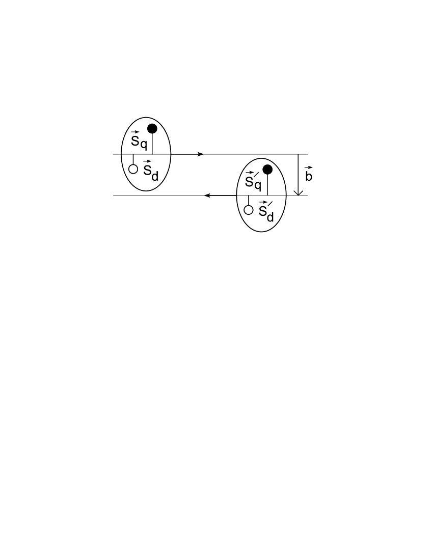
Figure 1: Proton-proton scattering in the quark-diquark model.

For the distribution of the constituents inside the nucleon we take a Gaussian with radius $R$:

$$D(s_{q},s_{d})=\frac{1+\lambda^{2}}{\pi R^{2}}e^{-(s_{q}^{2}+s_{d}^{2})/R^{2}}\delta^{2}(s_{d}+\lambda s_{q}).$$ (3)

The second parameter, $\lambda$, has the physical meaning of the ratio of the quark and diquark masses $\lambda=m_{q}/m_{d}$ (the delta function guarantees that the center-of-mass of the system moves along the straight line). One expects of course $1/2\leq\lambda\leq 1$.

Our strategy is to adjust the parameters of the model by demanding that (i) the total inelastic cross section (ii) the slope of the elastic cross section at $t=0$ (iii) the position of the first diffractive minimum in elastic cross section and (iv) the height of the second maximum in elastic scattering are in agreement with data.

The unitarity condition implies for the elastic amplitude

$$t_{el}(b)=1-\sqrt{1-\sigma(b)}.$$ (4)

The elastic amplitude in momentum transfer representation $T(\Delta)$ is a Fourier transform of the amplitude in impact parameter space:

$$T(\Delta)=\int t_{el}(b)e^{i\vec{\Delta}\cdot\vec{b}}d^{2}b=2\pi\int t_{el}(b)J_{0}(\Delta b)bdb,$$ (5)

where $J_{0}$ is the Bessel function.

With this normalization one can evaluate the relevant measurable quantities. Total cross section:

$$\sigma_{tot}=2T(0),$$ (6)

elastic differential cross section ($t\simeq-|\Delta|^{2}$):

$$\frac{d\sigma}{dt}=\frac{1}{4\pi}|T(\Delta)|^{2},$$ (7)

slope of the elastic cross section (at $t=0$):

$$B\equiv\frac{d}{dt}\left(\ln\frac{d\sigma}{dt}\right)|_{t=0}=\frac{\int t_{el}(b)b^{3}db}{2\int t_{el}(b)bdb}.$$ (8)

In the next sections we discuss two different choices for inelastic differential cross-sections of the constituents $\sigma_{ab}(s)$.

3 Diquark as a simple constituent

As a first choice we parametrized $\sigma_{ab}(s)$ using simple Gaussian forms:

$$\sigma_{ab}(s)=A_{ab}e^{-s^{2}/R_{ab}^{2}}.$$ (9)

The radii $R_{ab}$ were constrained by the condition $R_{ab}^{2}=R_{a}^{2}+R_{b}^{2}$ where $R_{a}$ denotes the quark or diquark’s radius (a natural constraint for the Gaussians).

This means that the quark and the diquark are treated on the same footing, their internal structures being described by one parameter, the radius ($R_{q}$ or $R_{d}$).

From (9) we deduce the total inelastic cross sections: $\sigma_{ab}=\pi A_{ab}R_{ab}^{2}$. To reduce the number of parameters, we also demand that the ratios of cross-sections satisfy the condition:

$$\sigma_{qq}:\sigma_{qd}:\sigma_{dd}=1:2:4,$$ (10)

expressing the idea that there are twice as many partons in the constituent diquark than those in the constituent quark (shadowing neglected). This allows to evaluate $A_{qd}$ and $A_{dd}$ in terms of $A_{qq}$:

$$A_{qd}=A_{qq}\frac{4R_{q}^{2}}{R_{q}^{2}+R_{d}^{2}},\quad A_{dd}=A_{qq}\frac{4R_{q}^{2}}{R_{d}^{2}}.$$ (11)

One sees that the model in this form contains $5$ parameters $R$, $\lambda$, $R_{q}$, $R_{d}$ and $A_{qq}$ (we expect $A_{qq}$ to be close to $1$).

Now the calculation of $\sigma(b)$ shown in (1) reduces to straightforward gaussian integrations. The relevant formula is given in the Appendix.

We have analyzed the data at all ISR energies [13, 14]. It turns out that the model works very well indeed, thus it is flexible enough. Note that this is not entirely trivial conclusion. For instance, an analogous calculation performed in the model with the assumption that the proton consists of three uncorrelated constituent quarks led to negative conclusions [6].

Four examples of our calculations are shown in Fig. 2, where the differential cross section $d\sigma/dt$ at the ISR energies $23$, $31$, $53$ and $62$ GeV, evaluated from the model, are compared with data [13].

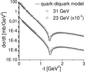
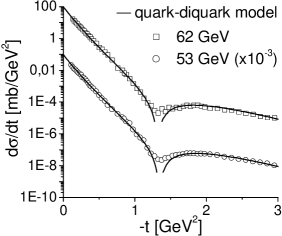
Figure 2: The quark-diquark model compared to data on differential cross section at four energies. Diquark as a simple constituent.

One sees an impressive agreement. Note that we are adjusting the model to account only for the slope and the value at $t=0$, and for the position of the minimum. Nevertheless, one sees that the resulting curve follows very well the subtle structure of the cross-section between $t=0$ and the minimum. This indicates that the nucleon model with two very different constituents may indeed represent more than a simple parametrization of data.

The values of the parameters at various energies are given in the Table 1. One sees some tendency for all radii to increase with increasing energy. Given the experimental and theoretical inaccuracies the effect is barely significant.

$\sqrt{s}$ [GeV]	$\lambda$	$R_{q}$ [fm]	$R_{d}$ [fm]	$R$ [fm]	$A_{qq}$
$23$	0.64	0.275	0.739	0.312	1
$31$	0.64	0.279	0.752	0.316	1
$53$	0.71	0.288	0.770	0.327	1
$62$	0.71	0.290	0.774	0.327	1

Table 1: Diquark as a simple constituent. The parameters of the model at four different energies.

The most striking feature seen in the Table 1 is the large value of the diquark radius $R_{d}$. It is almost three times larger than the radius of the quark, and not very much smaller than the radius of the proton itself. It is interesting that this feature agrees with other estimates [7], based on rather different arguments.

4 Diquark as a qq system

In this section we consider another option, treating the diquark as a system composed of the two constituent quarks. As before we parametrize $\sigma_{qq}(s)$ using the same simple Gaussian as in (9).

$$\sigma_{qq}(s)=A_{qq}e^{-s^{2}/2R_{q}^{2}}.$$ (12)

To evaluate quark-diquark and diquark-diquark cross-sections we need the distribution of the quarks inside the diquark which we again take as a Gaussian:

$$D(s_{q1},s_{q2})=\frac{1}{\pi d^{2}}e^{-\left(s_{q1}^{2}+s_{q2}^{2}\right)/2d^{2}}\delta^{2}(s_{q1}+s_{q2}),$$ (13)

where $s_{q1}$ and $s_{q2}$ are transverse positions of the quarks in the diquark.

Using the Glauber [12] and Czyz-Maximon [11] expansions, analogous to (1), we have:

$$\sigma_{qd}(s)=\frac{4A_{qq}R_{q}^{2}}{R_{d}^{2}+R_{q}^{2}}e^{-s^{2}\tfrac{1}{R_{d}^{2}+R_{q}^{2}}}-\frac{A_{qq}^{2}R_{q}^{2}}{R_{d}^{2}}e^{-s^{2}/R_{q}^{2}},$$ (14)

$$\sigma_{dd}(s) =\frac{4A_{qq}R_{q}^{2}}{R_{d}^{2}}e^{-s^{2}\tfrac{1}{2R_{d}^{2}}}-\frac{4A_{qq}^{2}R_{q}^{4}}{R_{d}^{4}}e^{-s^{2}/R_{d}^{2}}-\frac{2A_{qq}^{2}R_{q}^{2}}{2R_{d}^{2}-R_{q}^{2}}e^{-s^{2}/R_{q}^{2}}$$ (15)

$$+\frac{4A_{qq}^{3}R_{q}^{4}}{R_{d}^{2}(2R_{d}^{2}-R_{q}^{2})}e^{-s^{2}\tfrac{2R_{d}^{2}+R_{q}^{2}}{2R_{q}^{2}R_{d}^{2}}}-\frac{A_{qq}^{4}R_{q}^{4}}{(2R_{d}^{2}-R_{q}^{2})^{2}}e^{-s^{2}\tfrac{2}{R_{q}^{2}}},$$

where

$$R_{d}^{2}=d^{2}+R_{q}^{2}$$

is the effective diquark radius.

Introducing this result into the general formulae given in Section 2 one can evaluate the differential and total inelastic pp cross-sections.

Again we have analyzed the data at all ISR energies [13, 14]. It turns out that the model in this form also works reasonably well. The results are shown in Fig. 3, where the differential cross-section $d\sigma/dt$ at the various ISR energies (the same as in Fig. 2) are compared with the data. There is little difference between plots in Fig. 3 and that in Fig. 2, except the region $-t>2.5$ GeV² which is of no interest in the present context.

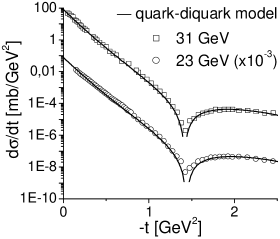
Figure 3: The quark-diquark model compared to data on differential cross section at four energies. Diquark as a $qq$ system.

The parameters used in Fig. 3 are given in Table 2.

$\sqrt{s}$ [GeV]	$\lambda$	$R_{q}$ [fm]	$R_{d}$ [fm]	$R$ [fm]	$A_{qq}$
$23$	1/2	0.322	0.748	0.154	0.78
$31$	1/2	0.327	0.761	0.157	0.78
$53$	1/2	0.335	0.781	0.161	0.79
$62$	1/2	0.336	0.786	0.163	0.80

Table 2: Diquark as a $qq$ system. The parameters of the model at four different energies.

One sees the similar features as in the model of Section 3. The diquark is much larger than the quark (confirming a weak binding), and the distance between quark and diquark even smaller than that in previous calculation.

From (12), (14) and (15) one can evaluate the total inelastic cross-section of the constituents. It turns out that the ratio of the cross-sections of the constituents satisfies:

$$\sigma_{qq}:\sigma_{qd}:\sigma_{dd}\approx 1:1.9:3.7,$$ (16)

which is rather close to (10), indicating a small amount of shadowing.

5 Discussion and conclusions

Our main conclusions can be summarized in three points.

(i) The constituent quark-diquark structure of the nucleon can account very well for the data on elastic $pp$ scattering at low momentum transfers and c. m. energies above $20$ GeV.

(ii) The confrontation with data allows to determine the parameters characterizing the two nucleon constituents.

(iii) The radius of the constituent diquark turns out much larger than that of the constituent quark. It is comparable to the radius of the nucleon.

Several comments are in order.

(a) It seems remarkable that our calculation reconstructs precisely the fine structure of the elastic scattering cross-section in the region before the first minimum. This indicates that, indeed, the two components of the proton with rather different radii are needed to explain the details of data.

(b) It is reassuring that our conclusion about the large radius of the diquark agrees with that obtained in [7] from rather different arguments.

(c) We have verified that the quark-diquark model gives also a good description of the $\pi p$ scattering. The discussion of this problem will be subject of a separate investigation [15].

(d) Finally, we find it significant that the quark-quark and quark-diquark cross-sections obtained here, when used in the wounded constituent model [10], explain very well the RHIC data on particle production in the central rapidity region.

Given all these arguments, it seems that the quark-diquark model of the nucleon structure at low momentum transfers does indeed capture the main features of this problem and thus deserves a closer attention.

Acknowledgements

We thank R. Peschanski, M. Praszalowicz and G. Ripka for discussions. This investigation was supported in part by the MEiN Grant No 1 P03 B 04529 (2005-2008).

6 Appendix

The presence of the two $\delta$ functions [c.f. (3)] reduces (1) to two gaussian integrations with the substitution

$$s_{d}=-\lambda s_{q};\quad s_{d}^{\prime}=-\lambda s_{q}^{\prime}.$$ (17)

The integration gives

$$\frac{4v^{2}}{\pi^{2}}\int d^{2}s_{q}d^{2}s_{q}^{\prime}e^{-2v(s_{q}^{2}+s_{q}^{\prime 2})}e^{-c_{qq}(b-s_{q}+s_{q}^{\prime})^{2}}e^{-c_{qd}(b-s_{q}+s_{d}^{\prime})^{2}}\times$$ (18)

$$\times e^{-c_{dq}(b-s_{d}+s_{q}^{\prime})^{2}}e^{-c_{dd}(b-s_{d}+s_{d}^{\prime})^{2}}=\frac{4v^{2}}{\Omega}e^{-b^{2}\Gamma/\Omega},$$

where:

$$\Omega =\left[4v+\left(1+\lambda\right)^{2}\left(c_{qd}+c_{dq}\right)\right]\left[v+c_{qq}+\lambda^{2}c_{dd}\right]+$$ (19)

$$+\left(1-\lambda\right)^{2}\left[v\left(c_{qd}+c_{dq}\right)+\left(1+\lambda\right)^{2}c_{qd}c_{dq}\right],$$

$$\Gamma =\left[4v+\left(1+\lambda\right)^{2}\left(c_{qd}+c_{dq}\right)\right]\left[v\left(c_{qq}+c_{dd}\right)+\left(1+\lambda\right)^{2}c_{qq}c_{dd}\right]+$$ (20)

$$+\left[4v+\left(1+\lambda\right)^{2}\left(c_{qq}+c_{dd}\right)\right]\left[v\left(c_{qd}+c_{dq}\right)+\left(1+\lambda\right)^{2}c_{qd}c_{dq}\right].$$

Other integrals can be obtained by putting some of the $c_{ab}=0$.

References

- [1] See, e.g., D. H. Perkins, Introduction to High Energy Physics, Cambridge U. Press (Cambridge, 2000).
- [2] See, e.g., H. J. Lipkin, F. Scheck, Phys. Rev. Lett. 16 (1966) 71; E. Levin, L. Frankfurt, JETP Lett. 2 (1965) 65; A. Bialas, K. Zalewski, Nucl. Phys. B6 (1968) 465.
- [3] A. Bialas, W. Czyz, W. Furmanski, Acta Phys. Pol. B8 (1977) 585; A. Bialas, W. Czyz, L. Lesniak, Phys. Rev. D25 (1982) 2328.
- [4] R. Nouicer, AIP Conf. Proc. 828 (2006) 11, nucl-ex/0512044; S. Eremin, S. Voloshin, Phys. Rev. C67 (2003) 064905; P. K. Netrakanti, B. Mohanty, Phys. Rev. C70 (2004) 027901; Bhaskar De, S. Bhattacharyya, Phys. Rev. C71 (2005) 024903. See also E. K. G. Sarkisyan, A. S. Sakharov, AIP Conf. Proc. 828 (2006) 35 and hep-ph/0410324 where the quark model is used to evaluate the energy deposition in the collision.
- [5] See, e.g., J. Bjorken, Acta Phys. Polon. B23 (1992) 637.
- [6] A. Bialas, K. Fialkowski, W. Slominski, M. Zielinski, Acta Phys. Pol. B8 (1977) 855.
- [7] See, e.g., R. Jaffe, F. Wilczek, Phys. World 17 (2004) 25; Phys. Rev. Lett. 91 (2003) 232003; M. Cristoforetti, P. Faccioli, G. Ripka, M. Traini, Phys. Rev. D71 (2005) 114010.
- [8] B. B. Back et al., Phys. Rev. C65 (2002) 061901; Phys. Rev. C70 (2004) 021902; Phys. Rev. C72 (2005) 031901; Phys. Rev. C74 (2006) 021901.
- [9] A. Bialas, M. Bleszynski, W. Czyz, Nucl. Phys. B111 (1976) 461.
- [10] A. Bialas, A. Bzdak, nucl-th/0611021.
- [11] W. Czyz, L. C. Maximon, Ann. of Phys. 52 (1969) 59.
- [12] R. J. Glauber, Lectures in Theoretical Physics, Vol. 1. Interscience, New York 1959.
- [13] E. Nagy et al., Nucl. Phys. B150 (1979) 221; N. Amos et al., Nucl. Phys. B262 (1985) 689; A. Breakstone et al., Nucl. Phys. B248 (1984) 253; A. Bohm et al., Phys. Lett. B49 (1974) 491.
- [14] U. Amaldi, K. R. Schubert, Nucl. Phys. B166 (1980) 301.
- [15] A. Bzdak, to be published.