CERN-PH-TH/2006-247 LPT–Orsay 06-78 TUM-HEP-653/06
Metastable Vacua in Flux Compactifications and Their Phenomenology

Abstract

In the context of flux compactifications, metastable vacua with a small positive cosmological constant are obtained by combining a sector where supersymmetry is broken dynamically with the sector responsible for moduli stabilization, which is known as the $F$–uplifting. We analyze this procedure in a model–independent way and study phenomenological properties of the resulting vacua.

1 Introduction

Recent progress in string theory compactifications with fluxes [1] has facilitated construction of string models with all moduli stabilized, zero or small cosmological constant, and broken supersymmetry. In the model of Kachru–Kallosh–Linde–Trivedi (KKLT) [2], the complex structure moduli and the dilaton are stabilized by fluxes on an internal manifold, while the Kähler ($T$) modulus is stabilized by non–perturbative effects such as gaugino condensation. The Kähler potential and the superpotential for the $T$–modulus are given by

$$K~{}=~{}-3\ln(T+\overline{T})\;,\quad W~{}=~{}W_{0}-A\,\mathrm{e}^{-a\,T}\;,$$ (1)

where $W_{0}$, $A$ and $a$ are model-dependent constants. Minimization of the corresponding scalar potential reveals that supersymmetry is unbroken at the minimum and the vacuum energy is negative and large in magnitude. To achieve a small and positive cosmological constant in this setup, KKLT introduced an anti–D3 brane whose contribution to vacuum energy can be adjusted arbitrarily. However, such a contribution breaks supersymmetry explicitly. It was later suggested in [3] that a similar uplifting effect could be achieved in the framework of spontaneously broken SUSY by including the $D$–terms. This procedure however cannot uplift the KKLT minimum due to the supergravity relation $D\propto F=0$ [4]. It can potentially be used to uplift non–SUSY minima such as those at exponentially large compactification volume [5, 6].

One of the obstacles to realizing the simplest KKLT scenario in supergravity is posed by the no–go theorem of Refs. [7, 8, 9] . It states that

if the modulus $T$ is the only light field and its Kähler potential is $K=-n\,\ln(T+\overline{T})$ ($1\leq n\leq 3$), de Sitter (dS) or Minkowski vacua with broken supersymmetry are not possible for any superpotential.

Thus, it is necessary to include additional fields in the system (or modify the Kähler potential [11]) providing the goldstino which is necessary to make the gravitino massive. In this case, dS or Minkowski vacua with spontaneously broken supersymmetry can be obtained due to the $F$–terms of hidden matter fields [9] (a somewhat similar approach was considered in [12]). Since matter fields are as generic as moduli in string constructions, this provides an interesting alternative to common scenarios with moduli/dilaton dominated SUSY breaking. In this article, we will follow our earlier work (LNR) [9].

Interest in this approach has been bolstered by recent work of Intriligator, Seiberg and Shih (ISS) [13] on dynamical SUSY breaking in metastable vacua. They have found that metastable vacua with broken supersymmetry are generic and realized even in simple systems like SUSY QCD. These vacua are long–lived and can be combined with the KKLT sector to achieve a small cosmological constant and acceptable supersymmetry breaking [14, 15, 16].

In this work, we analyze the $F$–term uplifting of the KKLT minimum in a model–independent way and study SUSY phenomenology of the resulting vacua. Before we proceed, let us give a few relevant supergravity formulae. The supergravity scalar potential is given by [17]

$$V~{}=~{}\mathrm{e}^{G}\,(G_{i}\,G_{\bar{\jmath}}\,G^{i\bar{\jmath}}-3)+{1\over 2}\,\operatorname{Re}(f_{a})^{-1}\,D^{a}D^{a}\;,$$ (2)

where $G=K+\ln|W|^{2}$ with $K$ and $W$ being the Kähler potential and the superpotential, respectively; $f_{a}$ is the gauge kinetic function, and $D^{a}$ are the $D$–terms. A subscript $i$ denotes differentiation with respect to the $i$-th field. $G^{i\bar{\jmath}}$ is the inverse Kähler metric. The gravitino mass is given by

$$m_{3/2}~{}=~{}\mathrm{e}^{G/2}\;,$$ (3)

and the SUSY–breaking $F$–terms are

$$F^{i}~{}=~{}\mathrm{e}^{G/2}\,G^{i\bar{\jmath}}\,G_{\bar{\jmath}}\;.$$ (4)

In what follows, we first review problems with the $D$–term uplifting and then focus on the uplifting with the $F$–terms.

2 Problems with the $\boldsymbol{D}$–term uplifting

There are two problems with the $D$–term uplifting scenario. First, supersymmetric minima cannot be uplifted by the $D$–terms [4]. The reason is that, in supergravity [17],

$$D^{a}\propto{1\over W}\,D_{i}W\;,$$ (5)

where $D_{i}W\equiv\partial_{i}W+W\partial_{i}K$. In supersymmetric configurations, $\langle D_{i}W\rangle=0$ and the $D$–terms vanish (unless $W=0$). Thus, only non–supersymmetric minima can potentially be uplifted.

Second, the $D$–term uplifting of non–supersymmetric vacua does not work either if the gravitino mass is hierarchically small [18] (unless moduli are exponentially large). Indeed, for matter on D7 branes, the gauge kinetic function is given by

$$f~{}=~{}T\;,$$ (6)

and the $D$–term of an anomalous U(1) is

$$D~{}\propto~{}{E\over\operatorname{Re}T}+\sum_{i}q_{i}\,|\phi_{i}|^{2}\;,$$ (7)

where $E$ is a constant related to the trace of the anomalous U(1) and $\phi_{i}$ are VEVs of fields carrying anomalous charges $q_{i}$. At the minimum of the scalar potential,

$$V_{T}~{}=~{}0\;,$$ (8)

which from Eq. (2) implies symbolically

$$m_{3/2}^{2}+D^{2}+D~{}=~{}0\;.$$ (9)

Here we have neglected all coefficients and assumed that there are no very large ($10^{15}$) or very small factors in this equation. Using $m_{3/2}\sim 10^{-15}$ (in Planck units) as favoured by phenomenology, this equation is solved by

$$D~{}\sim~{}m_{3/2}^{2}~{}\ll~{}m_{3/2}~{}\sim~{}F\;.$$ (10)

Thus, the $D$–term is much smaller than the $F$–terms and $D^{2}\sim m_{3/2}^{4}$ cannot uplift an AdS minimum with $V_{0}\sim-m_{3/2}^{2}$ to zero vacuum energy. This mechanism can only work for a heavy gravitino, e.g. $m_{3/2}\sim 1$. The existing examples of the $D$–term uplifting confirm this conclusion [19, 20, 21, 22] (for related work, see also [23, 24, 25]).

3 $\boldsymbol{F}$–term uplifting

It has been shown by LNR [9] that the $F$–term uplifting mechanism is viable and works for a hierarchically small gravitino mass. The $F$–uplifting in its simplest form amounts to combining a sector where supersymmetry is broken spontaneously in a metastable dS vacuum with the KKLT sector. Since the $T$–modulus is heavy, the resulting minimum of the system is given approximately by the minima in the separate subsectors. Then $T$ gives only a small contribution to SUSY breaking and the cosmological constant can be adjusted to be arbitrarily small. Let us study this procedure in more detail.

3.1 SUSY breaking sector

Consider a (hidden sector) matter field $\phi$ with

$$K~{}=~{}\overline{\phi}\phi\;,\quad W~{}=~{}\mathcal{W}(\phi)\;.$$ (11)

Suppose for simplicity that the minimum of the corresponding scalar potential

$$V~{}=~{}\mathrm{e}^{G}\,(G_{\phi}\,G_{\overline{\phi}}-3)\;,$$ (12)

is at real $\phi$. The non–supersymmetric minimum is found from

$$V_{\phi}~{}\propto~{}G_{\phi}^{2}+G_{\phi\phi}-2~{}=~{}0\;.$$ (13)

Denoting this minimum by $\phi_{0}$, supersymmetry is broken by $F^{\phi}~{}\sim~{}|\mathcal{W}|\,G_{\phi}\bigl{|}_{\phi_{0}}$. The vacuum energy can be chosen to be positive,

$$V(\phi_{0})~{}>~{}0\;,$$ (14)

and arbitrarily small by adjusting $\mathcal{W}(\phi)$. In this case, $F^{\phi}\sim|\mathcal{W}(\phi_{0})|$ and, assuming that the potential is not very steep, the mass of $\phi$ is typically of order $|\mathcal{W}(\phi_{0})|$.

3.2 KKLT sector

This sector consists of the $T$–modulus with the usual Kähler potential and the superpotential induced by fluxes and gaugino condensation,

$$K~{}=~{}-3\ln(T+\overline{T})\;,\quad W~{}=~{}\mathscr{W}(T)~{}\equiv~{}W_{0}-A\mathrm{e}^{-a\,T}\;,$$ (15)

with $A\sim 1$, $a\gg 1$. If the observable matter is placed on D7 branes, the SM gauge couplings require $\operatorname{Re}T\simeq 2$ at the minimum.

The scalar potential is

$$V~{}=~{}\mathrm{e}^{G}\,(G_{T}\,G_{\overline{T}}\,G^{T\overline{T}}-3)\;,$$ (16)

and its SUSY minimum is determined by

$$G_{T}~{}=~{}0\;.$$ (17)

The solution is

$$T_{0}~{}\approx~{}-{1\over a}\,\ln{W_{0}\over a}\;,$$ (18)

where again we have taken $T$ to be real. The corresponding vacuum energy is given by

$$V(T_{0})~{}=~{}-3\,\mathrm{e}^{G}\sim-\left|\mathscr{W}(T_{0})\right|^{2}\;.$$ (19)

3.3 KKLT + SUSY breaking sector

Now we combine the two sectors. The full Kähler potential and the superpotential are given by

$$K = |\phi|^{2}-3\ln(T+\overline{T})\;,$$

$$W = \mathcal{W}(\phi)+\mathscr{W}(T)\;.$$ (20)

The question is now how much the minimum of the system deviates from the minima of the separate subsectors.

Consider the system in the vicinity of the reference point $(\phi_{0},T_{0})$. At $T=T_{0}$, the superpotential for $\phi$ is

$$W~{}=~{}\mathcal{W}(\phi)+\mathscr{W}(T_{0})\;.$$ (21)

Similarly, at $\phi=\phi_{0}$ the superpotential for $T$ is

$$W~{}=~{}\mathscr{W}(T)+\mathcal{W}(\phi_{0})\;.$$ (22)

Thus, the constant terms in the superpotential shift relative to those of the original subsectors. It makes sense to compare the true minimum of the system to the minima of the subsectors with shifted superpotentials. For example, $T_{0}$ should be defined as the minimum of the KKLT subsector with the superpotential $\mathscr{W}(T)+\mathcal{W}(\phi_{0})$ and similarly for the $\phi$ subsector. This can be done iteratively.

The total potential is now

$$V~{}=~{}\mathrm{e}^{G}\,(G_{\phi}\,G_{\overline{\phi}}+G_{T}\,G_{\overline{T}}\,G^{T\overline{T}}-3)\;.$$ (23)

Let us see if $(\phi_{0},T_{0})$ is a stationary point. We have

$$V_{\phi} = G_{\phi}\,V+\mathrm{e}^{G}\,{\partial\over\partial\phi}(G_{\phi}G_{\overline{\phi}})+\mathrm{e}^{G}\,{\partial\over\partial\phi}(G_{T}\,G_{\overline{T}}\,G^{T\overline{T}})\;,$$

$$V_{T} = G_{T}\,V+\mathrm{e}^{G}\,{\partial\over\partial T}(G_{T}\,G_{\overline{T}}\,G^{T\overline{T}})+\mathrm{e}^{G}\,{\partial\over\partial T}(G_{\phi}\,G_{\overline{\phi}})\;.$$ (24)

Consider $V_{\phi}$. It is zero because the first two terms represent the equations of motion for the separate $\phi$–subsector, and the third term is proportional to $G_{T}$ which is zero at $T_{0}$. Consider now $V_{T}$. The first two terms are zero due to $G_{T}(T_{0})=0$. The last term however does not vanish,

$$\mathrm{e}^{G}\,{\partial\over\partial T}(G_{\phi}G_{\overline{\phi}})~{}\sim~{}m_{3/2}^{2}\;,$$ (25)

where we have used $G_{\phi},W_{T}/W\sim 1$ at $(\phi_{0},T_{0})$. It is non–zero but small compared to $V_{T\bar{T}}\sim a^{2}m_{3/2}^{2}$. Therefore, the (heavy) modulus shifts slightly from $T_{0}$. Finally, the vacuum energy at $(\phi_{0},T_{0})$ equals that of the $\phi$–subsector from Eq. (14).

We see that the stationary point conditions are “almost” satisfied at $(\phi_{0},T_{0})$. Let us now compute how much the true minimum is shifted compared to $(\phi_{0},T_{0})$. Suppose the true minimum is at $\phi_{0}+\delta\phi,T_{0}+\delta T$. At this point,

$$V_{\phi}(\phi_{0}+\delta\phi,T_{0}+\delta T) = 0\;,$$

$$V_{T}(\phi_{0}+\delta\phi,T_{0}+\delta T) = 0\;.$$ (26)

The $(\phi,T)$ system has been studied in detail in LNR [9], while here we will, for simplicity, treat $T$ and $\phi$ as real variables and expand this to first order in $\delta\phi,\delta T$,

$$V_{\phi\phi}\,\delta\phi+V_{\phi T}\,\delta T = 0\;,$$

$$V_{T}+V_{TT}\,\delta T+V_{T\phi}\,\delta\phi = 0\;,$$ (27)

where we have used $V_{\phi}(\phi_{0},T_{0})=0$ as explained above. The solution is

$$\delta T = {V_{T}\over V_{T\phi}^{2}/V_{\phi\phi}-V_{TT}}\;,$$

$$\delta\phi = -{V_{T\phi}\over V_{\phi\phi}}\,\delta T\;.$$ (28)

In the large $a$ limit, $\delta T\sim 1/a^{2}$ and $\delta\phi\sim 1/a~{}$.

Supersymmetry is now broken by $F^{\phi}$ and $F^{T}$ with the latter giving a small contribution,

$$F^{T}~{}\sim~{}\mathrm{e}^{G/2}\,{W_{TT}\over W}\,\delta T~{}\sim~{}{1\over a}\,m_{3/2}\;.$$ (29)

Finally, the cosmological constant can be chosen to be arbitrarily small by adjusting parameters of the $\phi$–subsector, i.e. ${\cal W}(\phi)$.

3.4 Example

As a simple example, consider a combination of the KKLT and the Polonyi model [27]. The superpotential of the Polonyi model is given by

$$\mathcal{W}(\phi)~{}=~{}c+\mu^{2}\,\phi\;,$$ (30)

where $c$ and $\mu^{2}$ are constants. A non–supersymmetric Polonyi vacuum is determined by

$$G_{\phi}^{2}+G_{\phi\phi}-2~{}=~{}0\;.$$ (31)

Choosing

$$G_{\phi}^{2}~{}=~{}3+\epsilon\;,$$ (32)

with $\epsilon\ll 1$, the vacuum energy is

$$V_{0}~{}\sim~{}\epsilon\,\mu^{4}\;.$$ (33)

The solution to first order in $\epsilon$ is given by

$$c~{}\approx~{}\mu^{2}\,\Bigl{(}2-\sqrt{3}-{\sqrt{3}\over 6}~{}\epsilon\Bigr{)}\;,\quad\phi~{}\approx~{}\sqrt{3}-1+{\sqrt{3}-3\over 6}\,\epsilon\;.$$ (34)

The mass of the Polonyi field is set by $\mu^{2}$.

Figure 1: Scalar potential of the KKLT + Polonyi model (in units of $10^{4}/\mu^{4}$).

This system can be used to uplift the AdS minimum of KKLT as explained above. Since $\mu^{2}\sim W_{0}$, the modulus is heavy compared to the Polonyi field. As a result, it shifts only slightly from the original position and its contribution to SUSY breaking is suppressed. The resulting vacuum energy can be made arbitrarily small by adjusting $\epsilon$ and without affecting other aspects of the system.

The scalar potential for $A=1$, $a=12$, $\mu=10^{-8}$ is displayed in Fig. 1.

3.5 Relation to ISS

An interesting class of matter sectors with dynamically broken supersymmetry is provided by ISS [13]. In this case, small $W_{0}$ is generated dynamically through dimensional transmutation. The ISS examples include SUSY QCD with massive flavours, whose dual is described by the superpotential

$$W~{}=~{}h\,\operatorname{Tr}\phi\,\Phi\,\widetilde{\phi}-h\,\mu^{2}\,\operatorname{Tr}\Phi\;.$$ (35)

Here $\phi_{i}^{a}$, $\widetilde{\phi}_{a}^{\bar{\jmath}}$, $\Phi^{i}_{\bar{\jmath}}$ are the quark and meson fields with $1\leq i,j\leq N_{f}$ and $1\leq a\leq N$ being the flavour and colour indices, respectively. $h$ and $\mu^{2}$ are (dynamically generated) constants.

This system possesses metastable vacua with broken supersymmetry and

$$V_{0}~{}=~{}(N_{f}-N)\,\left|h^{2}\,\mu^{4}\right|\;.$$ (36)

Such vacua can be used for uplifting the KKLT minimum along the lines described above. For more details, see [14, 15, 16].

3.6 Remark on other schemes

Although we have focused our discussion on uplifting the KKLT minimum, it is clear that very similar considerations apply to other schemes. Analogous systems arise in the heterotic string, with the substitution $K=-3\ln(T+\bar{T})\rightarrow-\ln(S+\bar{S})$ and $f=T\rightarrow S$. The analysis of SUSY breaking can be carried out in a similar fashion with the same qualitative conclusions.

A related analysis for M theory compactifications on $G_{2}$ manifolds is given in [28].

4 Soft terms

The resulting pattern of the soft terms is a version of the “matter dominated SUSY breaking” scenario [9]. $F$–term uplifting generally predicts heavy scalars with masses of order the gravitino mass and light gauginos,

$$m_{1/2}~{}\ll~{}m_{0}~{}\sim~{}m_{3/2}\;.$$ (37)

The suppression of the gaugino masses comes from the fact that the gauge kinetic function is independent of $\phi$ to leading order.

Let us now focus on the case $\langle\phi\rangle\ll 1$. Allowing for the Kähler potential coupling between $\phi$ and observable fields $Q_{i}$,

$$K~{}=~{}-3\ln(T+\overline{T})+\overline{\phi}\phi+\overline{Q}_{i}Q_{i}\,(T+\overline{T})^{n_{i}}\Bigl{[}1+\xi_{i}\,\overline{\phi}\phi+{\cal O}(\phi^{4})\Bigr{]}\;,$$ (38)

where $n_{i}$ are effective “modular weights”, we have [9]

$$M_{a} = M_{s}\,\left[\alpha_{\mathrm{FLM}}+b_{a}\,g_{a}^{2}\right]\;,$$ (39)

$$A_{ijk} = {}-M_{s}\,\left[3\,\alpha_{\mathrm{FLM}}-\gamma_{i}-\gamma_{j}-\gamma_{k}\right]\;,$$ (40)

$$m_{i}^{2} = (16\pi^{2}\,M_{s})^{2}\,\left[1-3\,\xi_{i}\right]\;,$$ (41)

with $M_{s}\equiv m_{3/2}/16\pi^{2}$. Here we follow the notation of [29]. $b_{a}$ and $\gamma_{i}$ are the beta–function coefficients and the anomalous dimensions, respectively. The gaugino masses and A–terms receive comparable contributions from the modulus and the anomaly [30, 31] as in Refs. [4, 32], while the scalar masses are dominated by the $F$–term of the uplifting field $\phi$. The parameter $\alpha_{\mathrm{FLM}}$ of [29] controls the balance between the modulus and the anomaly contributions to $M_{a}$ and $A_{ijk}$: at large $\alpha_{\mathrm{FLM}}$ the modulus contribution dominates, while at small $\alpha_{\mathrm{FLM}}$ the anomaly provides the dominant contribution.

The modular weights have little effect on the soft terms as they only affect the A–terms. Thus we have set them to zero. The important variables for phenomenology are $\alpha_{\mathrm{FLM}}$ and $\xi_{i}$.

An interesting feature of the soft terms is that the gaugino masses unify at a scale between the electroweak and the GUT scales [33] although there is no new physics appearing there. This is true in models where the non–universality in gaugino masses is given by the corresponding beta–functions. In general, loop–suppressed contributions to the gaugino masses come also from the Kähler anomalies [34, 35] and string threshold corrections [36]. When these are suppressed (e.g. when $\langle\phi\rangle\ll 1$), the “mirage unification” occurs. This, however, does not usually apply to the scalar masses.

In what follows, we study SUSY phenomenology of models with the pattern of soft terms given above.

5 Phenomenology

The variable string/GUT scale parameters in our scheme are

$$m_{3/2}~{}~{},~{}~{}\alpha_{\mathrm{FLM}}~{}~{},~{}~{}\xi_{i}~{}~{},~{}~{}\tan\beta\;,$$

while, for simplicity, we fix the sign of $\mu$ to be positive. Here $\xi_{i}$ can be different for Higgses and sfermions, but we assume it to be generation–independent. Further, we restrict ourselves to the range $0<\alpha_{\mathrm{FLM}}<30$ and $0\leq\xi_{i}<1/3$.

The “matter domination” scheme has distinct phenomenology. Compared to “mirage mediation” extensively studied in Refs. [4, 37, 33, 29, 38, 39, 40], our scenario differs in the scalar masses, which are now large and comparable to the gravitino mass. The controlled non–universality in the gaugino masses and the A–terms makes it different from mSUGRA and its extensions with non–universal Higgs masses. We find that there are considerable regions of parameter space where the scheme is consistent with all phenomenological constraints.

5.1 Constraints and observables

Certain regions of parameter space are excluded by absence of electroweak symmetry breaking and a charged/coloured LSP. Among other constraints, the most important ones come from the Higgs and chargino searches,

$$m_{h}~{}>~{}114\,\mathrm{GeV}\;,\quad m_{\tilde{\chi}^{+}}~{}>~{}103\,\mathrm{GeV}\;.$$ (42)

Due to heavy scalars in our scenario, we expect the lightest Higgs to be very similar to the SM Higgs, hence the LEP constraint $m_{h}>114\,\mathrm{GeV}$ applies. We further impose the $b\rightarrow s\gamma$ constraint from the B–factories [41, 42], $2.33\times 10^{-4}\leq\mathrm{BR}(b\rightarrow s\gamma)\leq 4.15\times 10^{-4}$.

We also take into account the dark matter constraint. That is, we assume that the LSP is stable, has thermal abundance and constitutes the dominant component of dark matter. Then we impose the $3\,\sigma$ WMAP constraint on dark matter abundance $0.087\lesssim\Omega_{\tilde{\chi}}\,h^{2}\lesssim 0.138$ [43] and exclude parts of parameter space. We also display parameter space allowed by a conservative bound $0.03<\Omega_{\tilde{\chi}}h^{2}<0.3$. Note that the above assumptions may be relaxed which would open up more available parameter space. For instance, the LSP abundance may be non–thermal or the LSP may only constitute a small component of dark matter.

Having singled out favoured regions of parameter space, we consider prospects of direct and indirect dark matter detection. Dark matter can be observed (“directly”) via elastic scattering on target nuclei with nuclear recoil (see [44, 45]). This process is dominated by the $Z$ and Higgs exchange. Indirect dark matter detection amounts to observing a gamma–ray flux from the Galactic center, which can be produced by dark matter annihilation [46, 47].

In our numerical analysis, we use the public codes SUSPECT [48], SOFTSUSY [49], DarkSUSY [50] and MicrOMEGAs [51].

5.2 Parameter space analysis

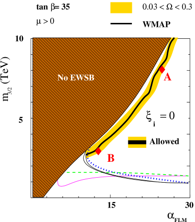
Figure 2: Allowed parameter space for tan$\beta=35$, $\xi_{i}=0$ and $\mu>0$. The region below the light grey (green) dashed line is excluded by the Higgs mass bound. The region below the the dotted line is excluded by the chargino mass bound, while that below the solid (magenta) line is excluded by BR($b\to s\gamma$). The narrow area between the black contours satisfies the $3\sigma$ WMAP constraint: $0.087\leq\Omega_{\tilde{\chi}_{1}^{0}}h^{2}\leq 0.138$, whereas the yellow region satisfies $0.03\leq\Omega_{\tilde{\chi}_{1}^{0}}h^{2}\leq 0.3$.

We start with the case $\xi_{i}=0$ and $\tan\beta=35$. The allowed parameter space is shown in Fig. 2, in yellow. The chargino and the Higgs mass constraints require $m_{3/2}$ to be above a few TeV. A large region is excluded due to no electroweak symmetry breaking (EWSB). This can be understood by writing the EWSB condition in terms of the GUT input parameters. At $\tan\beta=5$, we have [52]

$$M_{Z}^{2}~{}=~{}-1.8\,\mu^{2}-1.2\,m_{H_{u}}^{2}+5.9\,M_{3}^{2}+1.6\,m_{\tilde{q}_{3}}^{2}+\dots\;,$$ (43)

where $m_{\tilde{q}_{3}}$ is the third generation squark mass parameter. In the case of heavy scalars, the dominant contribution is given by $-1.2m_{H_{u}}^{2}+1.6m_{\tilde{q}_{3}}^{2}$, which must be positive. The coefficient of $m_{\tilde{q}_{3}}^{2}$ decreases with $\tan\beta$ due to the sbottom loops and at a certain critical value electroweak symmetry remains unbroken. Thus, at low $\tan\beta$ more parameter space is available.

Similarly, if we decrease the input value of $m_{\tilde{q}_{3}}^{2}$, electroweak symmetry gets restored. This means that increasing $\xi_{\mathrm{sf}}$ widens the region excluded by the “no EWSB” constraint.

The yellow region of Fig. 2 is favoured by dark matter considerations. There the LSP is a mixed higgsino–bino and the correct relic density is achieved due to neutralino annihilation and $\tilde{\chi}_{1}^{0}\tilde{\chi}_{1}^{+}$, $\tilde{\chi}_{1}^{0}\tilde{\chi}_{2}^{0}$ coannihilation processes. The sample spectra for this region are given in Table 1. To the left of the yellow region, the LSP relic density is below 0.03. This part of parameter space is also viable if the LSP constitutes only a fraction of dark matter. To the right of the yellow region, the relic density is too large. In principle, this could also be consistent with cosmological constraints if the dark matter production is non–thermal.

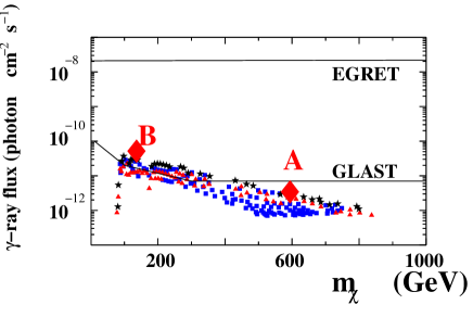
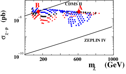
Figure 3: Scatter plot of the gamma-ray flux $\Phi_{\gamma}$ for a threshold of 1 GeV (left) and the spin–independent neutralino–proton cross section (right) as a function of the lightest neutralino mass $m_{\tilde{\chi}}$ for tan$\beta=35$, $\xi_{i}=0$ and $\mu>0$. An NFW dark matter profile with with $\Delta\Omega\sim 10^{-5}$ sr is used. All points in the figure satisfy the experimental bounds. The light grey (red) triangles correspond to $0.138<\Omega_{\tilde{\chi}^{0}_{1}}h^{2}<0.3$, black stars: $0.087<\Omega_{\tilde{\chi}^{0}_{1}}h^{2}<0.138$, dark grey (blue) boxes: $0.03<\Omega_{\tilde{\chi}^{0}_{1}}h^{2}<0.087$. The solid lines represent the $5\sigma$ sensitivity of the satellites.

Prospects for indirect and direct detection of dark matter are presented in Fig.3. Concerning the former, the gamma ray flux from the Galactic center is produced in this case by an s–channel $Z$ exchange or t–channel $\tilde{\chi}^{+}_{1},\tilde{\chi}_{2}^{0}$ exchange. We see that relatively light neutralinos, $m_{\tilde{\chi}^{0}_{1}}\lesssim 300$ GeV, can be detected by GLAST, a satellite based experiment to be launched in 2007, but are beyond the reach of EGRET. The neutralinos can also be detected directly via elastic scattering on nuclei dominated by the t–channel $Z$ and Higgs exchange. CDMS II (2007) will probe part of the parameter space, while ZEPLIN IV (2010) will cover the entire region allowed by WMAP. The scattering cross section is significant mainly due to the $Z$–exchange contribution and the higgsino–bino nature of the neutralino.

A B $\tan\beta$ 35 35 $\alpha$ 23.8 11.9 $m_{3/2}$ (TeV) 8 3 $M_{1}$ 625 125 $M_{2}$ 999 187 $M_{3}$ 2267 430 $m_{\tilde{\chi}^{0}_{1}}$ 594 112 $m_{\tilde{\chi}^{0}_{2}}$ 635 159 $m_{\tilde{\chi}^{+}_{1}}$ 627 151 $m_{\tilde{g}}$ 2810 612 $m_{h}$ 127.1 121.1 $m_{A}$ 5972 2236 $m_{H}$ 5972 2236 $\mu$ 617 194 $m_{\tilde{t}_{1}}$ 4483 1732 $m_{\tilde{t}_{2}}$ 5477 2239 $m_{\tilde{c}_{1}},~{}m_{\tilde{u}_{1}}$ 8171 2293 $m_{\tilde{c}_{2}},~{}m_{\tilde{u}_{2}}$ 8172 2989 $m_{\tilde{b}_{1}}$ 6240 2241 $m_{\tilde{b}_{2}}$ 7249 2647 $m_{\tilde{s}_{1}},~{}m_{\tilde{d}_{1}}$ 8170 2984 $m_{\tilde{s}_{2}},~{}m_{\tilde{d}_{2}}$ 8172 2994 $m_{\tilde{\tau}_{1}}$ 7098 2657 $m_{\tilde{\tau}_{2}}$ 7568 2825 $m_{\tilde{\mu}_{1}},~{}m_{\tilde{e}_{1}}$ 8001 2989 $m_{\tilde{\mu}_{2}},~{}m_{\tilde{e}_{2}}$ 8003 2996 $m_{\tilde{\nu}_{3}}$ 8003 2988 $\Omega h^{2}$ 0.108 0.101

Table 1: Sample spectra. All masses are in GeV, except for $m_{3/2}$ (in TeV).

5.3 Dependence on $\boldsymbol{\tan\beta}$ and $\boldsymbol{\xi_{i}}$

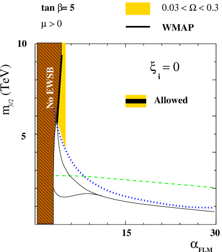
Figure 4: The same as in Fig. 2 but with tan$\beta=5$.

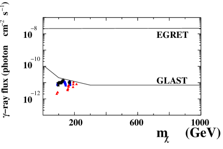
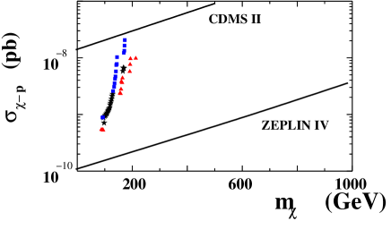
Figure 5: The same as in Fig. 3 but for tan$\beta=5$.

For lower $\tan\beta$, the “no EWSB” constraint relaxes, as explained above. The allowed region is again on the edge of the “no EWSB” area (Fig. 4). An interesting feature, absent in mSUGRA, is that $M_{1}(M_{Z})\simeq M_{2}(M_{Z})$ is possible. In this case, strong coannihilation of bino–neutralinos with wino–charginos ($m_{\tilde{\chi}_{1}^{0}}\sim m_{\tilde{\chi}_{1}^{+}}$) gives the relic LSP density consistent with WMAP. On the other hand, the indirect and direct detection rates are somewhat lower (Fig. 5). The neutralinos and charginos are light ($\lesssim 200$ GeV) and can be produced in collider experiments.

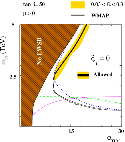
Figure 6: The same as in Fig. 2 but for tan$\beta=50$.

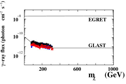
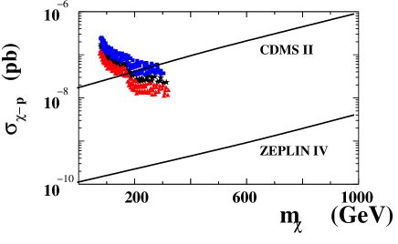
Figure 7: The same as in Fig. 3 but for tan$\beta=50$.

At $\tan\beta\sim 50$, the picture is similar to the $\tan\beta=35$ case (Fig. 6) except the detection rates are now enhanced (Fig. 7). We do not observe the A–pole funnel for dark matter annihilation since the scalars are too heavy in the considered parameter space.

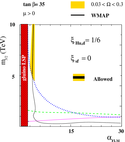
Figure 8: The same as in Fig. 2 but for $\xi_{H_{i}}=1/6$, $\xi_{\tilde{f}}=0$.

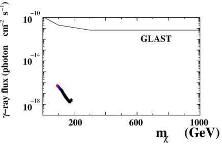
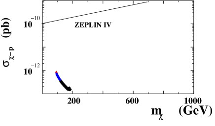
Figure 9: The same as in Fig. 3 but for $\xi_{H_{i}}=1/6$, $\xi_{\tilde{f}}=0$.

Increasing $\xi_{H_{u,d}}$ eliminates the “no EWSB” region (Fig. 8), as is clear from Eq.(43). In this case, a gluino LSP region appears at small $\alpha_{\mathrm{FLM}}$. Now the WMAP constraint is satisfied for larger $\mu$ and the LSP is a bino–wino. Consequently, the detection rates are suppressed (Fig. 9).

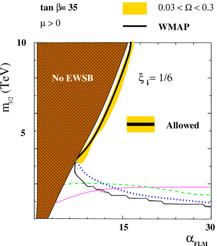
Figure 10: The same as in Fig. 2 but for $\xi_{i}=1/6$.

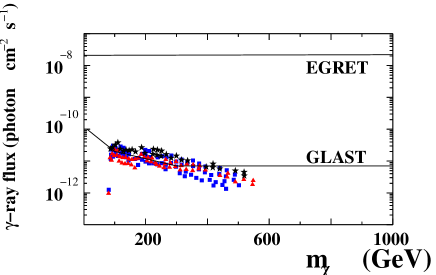
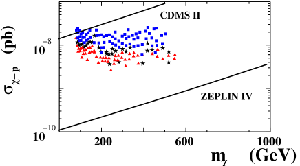
Figure 11: The same as in Fig. 3 but for $\xi_{i}=1/6$.

For all $\xi_{i}=1/6$, we essentially recover the plots for $\xi_{i}=0$ and the same conclusions (Figs. 10,11).

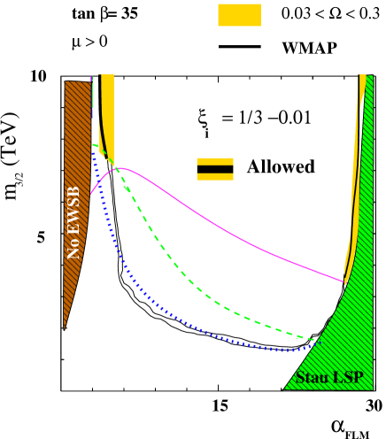
Figure 12: The same as in Fig. 2 but for $\xi_{i}=1/3-10^{-2}$.

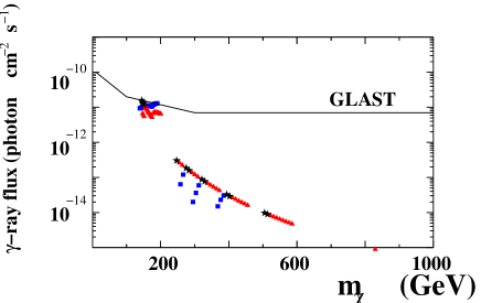
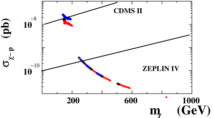
Figure 13: The same as in Fig. 3 but for $\xi_{i}=1/3-10^{-2}$.

Making the scalars lighter, $\xi_{i}=1/3-10^{-2}$, changes the picture dramatically (Fig. 12). The stau can be the LSP, similarly to the mSUGRA case. Close to the stau LSP region, $\tilde{\chi}^{0}_{1}\tilde{\tau}_{1}$ coannihilation is efficient and allows for an extra band in the parameter space consistent with WMAP. In this region, $\tilde{\chi}^{0}_{1}$ is mainly a bino and the detection rates are suppressed (Fig. 13). The points with significant detection rates correspond to the band on the left hand side of Fig. 12, in which case $\tilde{\chi}^{0}_{1}$ is a mixed higgsino–bino.

For $\xi_{i}=1/3$, we recover the “mirage mediation” soft terms [4], in which case the (suppressed) anomaly and modulus contributions to the scalar masses have to be included. The corresponding parameter space analysis can be found in [29, 40].

5.4 Summary

The “matter domination” scenario differs from the “mirage mediation” scheme and mSUGRA in several phenomenological aspects. First, the scalars are usually much heavier than the gauginos. This exacerbates the MSSM finetuning problem on one hand, but reduces the finetuning needed to suppress excessive CP violation and FCNC, on the other hand. The gauginos and higgsinos are typically quite light and accessible to collider searches. The neutralino dark matter can also be detected via the gamma ray flux from the Galactic center as well as elastic scattering on nuclei.

The typical values of $\alpha_{\mathrm{FLM}}$ increase compared to mirage mediation due to the electroweak symmetry breaking constraint. Also there are no charged or coloured tachyons. Non–universality in gaugino masses allows for $M_{1}(M_{Z})\simeq M_{2}(M_{Z})$, which is not possible in mSUGRA and leads to efficient chargino–neutralino coannihilation.

6 Comments on cosmological problems

The class of models we study do not offer an immediate solution to the gravitino or moduli problems [53]. The main point of these problems is that late decaying particles like gravitinos and moduli spoil the standard nucleosynthesis (BBN), which has proven to be very successful. One way to avoid these problems is to make gravitinos and moduli sufficiently heavy, 40 TeV or so, such that they decay before the BBN. This is possible in our framework for the price of increasing the sfermion masses as well. We note, however, that the above estimate is based on the decay width

$$\Gamma~{}\sim~{}\frac{m_{\mathrm{scalar}}^{3}}{M^{2}}\;,$$ (44)

with $M\sim M_{\mathrm{Pl}}$. In practice, this identification may be too rough and, depending on the Kähler potential and other factors, $M$ can be close to $M_{\mathrm{GUT}}$. In this case, the moduli problem is less severe and would not require a significant increase in the scalar mass. In such a scenario, the late–time entropy production will change the picture of dark matter generation (cf. [54]).

A version of the above problem, the so called “moduli–induced gravitino problem”, was recently pointed out in the context of the KKLT model with the anti-D3 brane uplifting [55, 56]. In this setup, supersymmetry is broken explicitly and $m_{T}\gg m_{3/2}$. As a result, the branching ratio for the $T$ decays into gravitinos is of order one which leads to abundant gravitino production and severe cosmological problems. In the context of spontaneously broken supergravity, such a problem is usually absent [9, 57] since the uplifting field $\phi$ typically has a mass comparable to $m_{3/2}$,

$$m_{\phi}\sim{\cal O}(m_{3/2})\;.$$ (45)

This is because, unlike $W(T)$, the uplifting superpotential is not very steep [14, 15, 16]. $\phi$ dominates the energy–density of the Universe at late times, however its decay into gravitinos is suppressed and the “moduli–induced gravitino problem” is absent.

7 Conclusions

Obtaining phenomenologically interesting vacua in flux compactifications is a difficult task. One of the problems is that the simple models such as the KKLT predict the existence of a deep AdS vacuum which then has to be “uplifted” to a dS/Minkowski vacuum by some mechanism. Here we have advocated the possibility that such uplifting can be provided by hidden matter $F$–terms, along the lines of our earlier work [9]. In this case, vacua with spontaneously broken supersymmetry, small positive cosmological constant and hierarchically small $m_{3/2}$ can be obtained. This procedure leads to “matter dominated” supersymmetry breaking, with the modulus contribution being suppressed. The resulting soft masses are characterized by light gauginos and heavy scalars.

We have performed a parameter space analysis in this class of models. There are considerable portions of parameter space consistent with all of the experimental constraints and accessible to collider searches. We also find good prospects for direct and indirect detection of neutralino dark matter in the near future.

Acknowledgements. This work was partially supported by the European Union 6th framework program MRTN-CT-2004-503069 “Quest for unification”, MRTN-CT-2004-005104 “ForcesUniverse”, MRTN-CT-2006-035863 “UniverseNet” and SFB-Transregio 33 “The Dark Universe” by Deutsche Forschungsgemeinschaft (DFG). The work of Y.M. is sponsored by the PAI program PICASSO under contract PAI–10825VF.

References

- [1] S. B. Giddings, S. Kachru, and J. Polchinski, Phys. Rev. D66 (2002), 106006, [hep-th/0105097].
- [2] S. Kachru, R. Kallosh, A. Linde, and S. P. Trivedi, Phys. Rev. D68 (2003), 046005, [hep-th/0301240].
- [3] C. P. Burgess, R. Kallosh, and F. Quevedo, JHEP 10 (2003), 056, [hep-th/0309187].
- [4] K. Choi, A. Falkowski, H. P. Nilles, and M. Olechowski, Nucl. Phys. B718 (2005), 113–133, [hep-th/0503216].
- [5] V. Balasubramanian, P. Berglund, J. P. Conlon, and F. Quevedo, JHEP 03 (2005), 007, [hep-th/0502058].
- [6] J. P. Conlon, S. S. Abdussalam, F. Quevedo, and K. Suruliz, (2006), hep-th/0610129.
- [7] R. Brustein and S. P. de Alwis, Phys. Rev. D69 (2004), 126006, [hep-th/0402088].
- [8] M. Gomez-Reino and C. A. Scrucca, JHEP 05 (2006), 015, [hep-th/0602246].
- [9] O. Lebedev, H. P. Nilles, and M. Ratz, Phys. Lett. B636 (2006), 126, [hep-th/0603047].
- [10] D. Lüst, S. Reffert, E. Scheidegger, W. Schulgin and S. Stieberger, arXiv:hep-th/0609013.
- [11] S. P. de Alwis, Phys. Lett. B 626, 223 (2005) [hep-th/0506266].
- [12] A. Saltman and E. Silverstein, JHEP 11 (2004), 066, [hep-th/0402135].
- [13] K. Intriligator, N. Seiberg, and D. Shih, JHEP 04 (2006), 021, [hep-th/0602239].
- [14] E. Dudas, C. Papineau, and S. Pokorski, (2006), hep-th/0610297.
- [15] H. Abe, T. Higaki, T. Kobayashi, and Y. Omura, (2006), hep-th/0611024.
- [16] R. Kallosh and A. Linde, (2006), hep-th/0611183.
- [17] E. Cremmer, S. Ferrara, L. Girardello and A. Van Proeyen, Nucl. Phys. B 212, 413 (1983).
- [18] K. Choi and K. S. Jeong, JHEP 08 (2006), 007, [hep-th/0605108].
- [19] G. Villadoro and F. Zwirner, Phys. Rev. Lett. 95 (2005), 231602, [hep-th/0508167].
- [20] A. Achucarro, B. de Carlos, J. A. Casas, and L. Doplicher, JHEP 06 (2006), 014, [hep-th/0601190].
- [21] S. L. Parameswaran and A. Westphal, JHEP 10 (2006), 079, [hep-th/0602253].
- [22] E. Dudas and Y. Mambrini, JHEP 10 (2006), 044, [hep-th/0607077].
- [23] F. Brümmer, A. Hebecker, and M. Trapletti, Nucl. Phys. B755 (2006), 186–198, [hep-th/0605232].
- [24] M. Haack, D. Krefl, D. Lüst, A. Van Proeyen, and M. Zagermann, (2006), hep-th/0609211.
- [25] A. P. Braun, A. Hebecker, and M. Trapletti, (2006), hep-th/0611102.
- [26] D. Lüst, S. Reffert and S. Stieberger, Nucl. Phys. B 727, 264 (2005) [arXiv:hep-th/0410074].
- [27] J. Polonyi, (1977), Budapest preprint KFK-1977-93.
- [28] B. Acharya, K. Bobkov, G. Kane, P. Kumar and D. Vaman, Phys. Rev. Lett. 97 (2006) 191601 [arXiv:hep-th/0606262].
- [29] A. Falkowski, O. Lebedev, and Y. Mambrini, JHEP 0511, 034 (2005) [hep-ph/0507110].
- [30] L. Randall and R. Sundrum, Nucl. Phys. B557 (1999), 79–118, [hep-th/9810155].
- [31] G. F. Giudice, M. A. Luty, H. Murayama, and R. Rattazzi, JHEP 12 (1998), 027, [hep-ph/9810442].
- [32] K. Choi, A. Falkowski, H. P. Nilles, M. Olechowski and S. Pokorski, JHEP 0411, 076 (2004) [hep-th/0411066].
- [33] K. Choi, K. S. Jeong, and K.-i. Okumura, JHEP 0509, 039 (2005) [hep-ph/0504037].
- [34] J. A. Bagger, T. Moroi, and E. Poppitz, JHEP 04 (2000), 009, [hep-th/9911029].
- [35] P. Binetruy, M. K. Gaillard and B. D. Nelson, Nucl. Phys. B 604, 32 (2001) [hep-ph/0011081].
- [36] L. J. Dixon, V. Kaplunovsky, and J. Louis, Nucl. Phys. B355 (1991), 649–688.
- [37] M. Endo, M. Yamaguchi and K. Yoshioka, Phys. Rev. D 72, 015004 (2005) [hep-ph/0504036].
-
[38]
K. Choi, K. S. Jeong, T. Kobayashi and K. i. Okumura,
Phys. Lett. B 633, 355 (2006)
[hep-ph/0508029];
R. Kitano and Y. Nomura, Phys. Lett. B 631, 58 (2005) [hep-ph/0509039];
O. Lebedev, H. P. Nilles and M. Ratz, hep-ph/0511320;
A. Pierce and J. Thaler, JHEP 0609, 017 (2006) [hep-ph/0604192]. - [39] O. Loaiza-Brito, J. Martin, H. P. Nilles and M. Ratz, AIP Conf. Proc. 805, 198 (2006) [hep-th/0509158].
-
[40]
H. Baer, E. K. Park, X. Tata and T. T. Wang,
JHEP 0608, 041 (2006)
[hep-ph/0604253];
Phys. Lett. B 641, 447 (2006) [hep-ph/0607085];
K. Choi, K. Y. Lee, Y. Shimizu, Y. G. Kim and K. i. Okumura, hep-ph/0609132. - [41] S. Chen et al. [CLEO Collaboration], Phys. Rev. Lett. 87, 251807 (2001) [hep-ex/0108032].
- [42] H. Tajima [BELLE Collaboration], Int. J. Mod. Phys. A17, 2967 (2002) [hep-ex/0111037].
- [43] D. N. Spergel et al., astro-ph/0603449.
- [44] C. Muñoz, Int. J. Mod. Phys. A 19, 3093 (2004) [hep-ph/0309346].
- [45] G. Bertone, D. Hooper and J. Silk, Phys. Rept. 405, 279 (2005) [hep-ph/0404175].
-
[46]
F. Prada, A. Klypin, J. Flix, M. Martinez and E. Simonneau,
astro-ph/0401512;
G. Bertone and D. Merritt, Mod. Phys. Lett. A 20, 1021 (2005) [astro-ph/0504422];
Y. Mambrini, C. Munoz, E. Nezri and F. Prada, JCAP 0601, 010 (2006) [arXiv:hep-ph/0506204]. -
[47]
D. Hooper, I. de la Calle Perez, J. Silk, F. Ferrer and S. Sarkar,
JCAP 0409, 002 (2004)
[astro-ph/0404205];
Y. Mambrini and C. Muñoz, Astropart. Phys. 24, 208 (2005) [hep-ph/0407158];
JCAP 0410, 003 (2004) [hep-ph/0407352];
S. Profumo, Phys. Rev. D 72, 103521 (2005) [astro-ph/0508628];
H. Baer, A. Mustafayev, E. K. Park, S. Profumo and X. Tata, JHEP 0604, 041 (2006) [hep-ph/0603197]. -
[48]
A. Djouadi, J. L. Kneur and G. Moultaka,
hep-ph/0211331;
http://www.lpm.univ-montp2.fr:6714/~kneur/suspect.html. - [49] B. C. Allanach, Comput. Phys. Commun. 143, 305 (2002) [hep-ph/0104145].
-
[50]
P. Gondolo, J. Edsjo, P. Ullio, L. Bergstrom, M. Schelke and E. A.
Baltz, astro-ph/0406204;
http://www.physto.se/~edsjo/darksusy. -
[51]
G. Belanger, F. Boudjema, A. Pukhov and A. Semenov,
hep-ph/0607059;
Comput. Phys. Commun. 149, 103 (2002) [hep-ph/0112278]. - [52] G. L. Kane, J. D. Lykken, B. D. Nelson and L. T. Wang, Phys. Lett. B 551, 146 (2003) [hep-ph/0207168].
- [53] G. D. Coughlan et al., Phys. Lett. B158 (1985), 401.
- [54] M. Drees, H. Iminniyaz and M. Kakizaki, Phys. Rev. D 73, 123502 (2006) [hep-ph/0603165].
- [55] M. Endo, K. Hamaguchi, and F. Takahashi, Phys. Rev. Lett. 96, 211301 (2006) [hep-ph/0602061].
- [56] S. Nakamura and M. Yamaguchi, Phys. Lett. B 638, 389 (2006)[arXiv:hep-ph/0602081].
- [57] M. Dine, R. Kitano, A. Morisse, and Y. Shirman, Phys. Rev. D73 (2006), 123518 [hep-ph/0604140].