Neutrino Masses, Lepton Flavor Mixing and Leptogenesis
in the Minimal Seesaw Model

Abstract

We present a review of neutrino phenomenology in the minimal seesaw model (MSM), an economical and intriguing extension of the Standard Model with only two heavy right-handed Majorana neutrinos. Given current neutrino oscillation data, the MSM can predict the neutrino mass spectrum and constrain the effective masses of the tritium beta decay and the neutrinoless double-beta decay. We outline five distinct schemes to parameterize the neutrino Yukawa-coupling matrix of the MSM. The lepton flavor mixing and baryogenesis via leptogenesis are investigated in some detail by taking account of possible texture zeros of the Dirac neutrino mass matrix. We derive an upper bound on the CP-violating asymmetry in the decay of the lighter right-handed Majorana neutrino. The effects of the renormalization-group evolution on the neutrino mixing parameters are analyzed, and the correlation between the CP-violating phenomena at low and high energies is highlighted. We show that the observed matter-antimatter asymmetry of the Universe can naturally be interpreted through the resonant leptogenesis mechanism at the TeV scale. The lepton-flavor-violating rare decays, such as $\mu\to e+\gamma$, are also discussed in the supersymmetric extension of the MSM.

1 Introduction

Recent solar,[1] atmospheric,[2] reactor[3] and accelerator[4] neutrino oscillation experiments have provided us with very robust evidence that neutrinos are massive and lepton flavors are mixed. This great breakthrough opens a novel window to new physics beyond the Standard Model (SM). In order to generate neutrino masses, the most straightforward extension of the SM is to preserve its $SU(2)_{\rm L}\times U(1)_{\rm Y}$ gauge symmetry and introduce a right-handed neutrino for each lepton family. Neutrinos can therefore acquire masses via the Dirac mass term, which links the lepton doublets to the right-handed singlets. If we adopt such a scenario and confront the masses of Dirac neutrinos with current experimental data, we have to give a reasonable explanation for the extremely tiny neutrino Yukawa couplings. This unnaturalness can be overcome, however, provided neutrinos are Majorana particles instead of Dirac particles. In this case, it is also possible to write out a lepton-number-violating mass term in terms of the fields of right-handed Majorana neutrinos. Since the latter are $SU(2)_{\rm L}$ singlets, their masses are not subject to the spontaneous gauge symmetry breaking. Given the Dirac neutrino mass term of the same order as the electroweak scale $\Lambda_{\rm EW}\sim 10^{2}$ GeV, the small masses of left-handed Majorana neutrinos can be generated by pushing the masses of right-handed Majorana neutrinos up to a superhigh-energy scale close to the scale of grand unified theories $\Lambda_{\rm GUT}\sim 10^{16}~{}{\rm GeV}$. This is just the well-known seesaw mechanism,[5] which has been extensively discussed in the literature. There are of course some other ways to make neutrinos massive. For instance, one may extend the SM with the scalar singlets or triplets which couple to two lepton doublets and form a gauge invariant mass term.[6] Neutrinos can then gain the Majorana masses after the relevant scalars gain their vacuum expectation values. But why is the seesaw mechanism so attractive? An immediate answer to this question is that the seesaw mechanism can not only account for the smallness of neutrino masses in a natural way, but also provide a natural possibility to interpret the observed matter-antimatter asymmetry of the Universe.

The cosmological baryon-antibaryon asymmetry is a long-standing problem in particle physics and cosmology. To dynamically generate a net baryon number asymmetry in the Universe, three Sakharov conditions have to be satisfied:[7] (1) baryon number non-conservation; (2) C and CP violation; (3) a departure from thermal equilibrium. Fortunately, both $B$- and $L$-violating anomalous interactions exist in the SM and can be in thermal equilibrium when the temperature is much higher than the electroweak scale. Fukugita and Yanagida have pointed out that it is possible to understand baryogenesis by means of the mechanism of leptogenesis,[8] in which a net lepton number asymmetry is generated from the CP-violating and out-of-equilibrium decays of heavy right-handed Majorana neutrinos. This lepton number asymmetry is partially converted into the baryon number asymmetry via the $(B-L)$-conserving sphaleron interaction,[9] such that the matter-antimatter asymmetry comes into being in the Universe.

The fact of neutrino oscillations and the elegance of leptogenesis convince us of the rationality of the seesaw mechanism. However, the seesaw models are usually pestered with too many parameters. In the framework of the SM extended with three right-handed Majorana neutrinos, for instance, there are fifteen free parameters in the Dirac Yukawa couplings as well as three unknown mass eigenvalues of heavy Majorana neutrinos. But the effective neutrino mass matrix resulting from the seesaw relation contains only nine physical parameters. That is to say, specific assumptions have to be made for the model so as to get some testable predictions for the neutrino mass spectrum, neutrino mixing angles and CP violation. Among many realistic seesaw models existing in the literature, the most economical one is the so-called minimal seesaw model (MSM) proposed by Frampton, Glashow and Yanagida.[10] The MSM contains only two right-handed Majorana neutrinos, hence the number of its free parameters is eleven instead of eighteen. Motivated by the simplicity and predictability of the MSM, a number of authors have explored its phenomenology. In particular, the following topics have been investigated: (a) the neutrino mass spectrum and its implication on the tritium beta decay and the neutrinoless double-beta decay; (b) specific neutrino mass matrices and their consequences on lepton flavor mixing and CP violation in neutrino oscillations; (c) radiative corrections to the neutrino mass and mixing parameters from the seesaw scale to the electroweak scale; (d) baryogenesis via leptogenesis at a superhigh-energy scale or via resonant leptogenesis[11] at the TeV scale; (e) lepton-flavor-violating processes (e.g., $\mu\to e+\gamma$) in the minimal supersymmetric extension of the SM. The purpose of this article is just to review a variety of works on these topics in the framework of the MSM.

The remaining parts of this review are organized as follows. In Sec. 2, we first describe the main features of the MSM and its minimal supersymmetric extension, and then discuss the neutrino mass spectrum and the lepton flavor mixing pattern. Stringent constraints are obtained on the effective masses of the tritium $\beta$ decay and the neutrinoless double-$\beta$ decay. Sec. 3 is devoted to a summary of five distinct parameterizations of the Dirac neutrino Yukawa couplings. They will be helpful for us to gain some insight into physics at high energies, when the relevant parameters are measured or constrained at low energies. In Sec. 4, we present a phenomenological analysis of the MSM with specific texture zeros in its Dirac Yukawa coupling matrix. Neutrino masses, lepton flavor mixing angles and CP-violating phases are carefully analyzed for the two-zero textures, in which the renormalization-group running effects on the neutrino mixing parameters are also calculated. Assuming the masses of two heavy right-handed Majorana neutrinos to be hierarchical, we derive an upper bound on the CP-violating asymmetry in the decay of the lighter right-handed Majorana neutrino in Sec. 5. We present a resonant leptogensis scenario at the TeV scale and a conventional leptogenesis scenario at much higher energy scales to interpret the cosmological baryon-antibaryon asymmetry. The correlation between the CP-violating phenomena at high and low energies is highlighted. For completeness, we also give some brief discussions about the lepton-flavor-violating processes $l_{j}\to l_{i}+\gamma$ in the supersymmetric MSM. In Sec. 6, we draw a number of conclusions and remark the importance of the MSM as an instructive example for model building in neutrino physics.

2 The Minimal Seesaw Model (MSM)

2.1 Salient Features of the MSM

In the MSM, two heavy right-handed Majorana neutrinos $N^{~{}}_{i\rm R}$ (for $i=1,2$) are introduced as the $SU(2)_{\rm L}$ singlets. The Lagrangian relevant for lepton masses can be written as[10]

$$-{\cal L}_{\rm lepton}\;=\;\overline{l^{~{}}_{\rm L}}Y^{~{}}_{l}E^{~{}}_{\rm R}H+\overline{l^{~{}}_{\rm L}}Y^{~{}}_{\nu}N^{~{}}_{\rm R}\tilde{H}+\frac{1}{2}\overline{N^{\rm c}_{\rm R}}M^{~{}}_{\rm R}N^{~{}}_{\rm R}+{\rm h.c.}\;,$$ (2.1)

where $\tilde{H}\equiv i\sigma^{~{}}_{2}H^{*}$ and $l_{\rm L}$ denotes the left-handed lepton doublet, while $E^{~{}}_{\rm R}$ and $N^{~{}}_{\rm R}$ stand respectively for the right-handed charged-lepton and neutrino singlets. After the spontaneous gauge symmetry breaking, one obtains the charged-lepton mass matrix $M^{~{}}_{l}=vY^{~{}}_{l}$ and the Dirac neutrino mass matrix $M^{~{}}_{\rm D}=vY^{~{}}_{\nu}$ with $v\simeq 174~{}{\rm GeV}$ being the vacuum expectation value (vev) of the neutral component of the Higgs doublet $H$. The heavy right-handed Majorana neutrino mass matrix $M^{~{}}_{\rm R}$ is a $2\times 2$ symmetric matrix. The overall lepton mass term turns out to be

$$-{\cal L}_{\rm mass}\;=\;\overline{E^{~{}}_{\rm L}}M^{~{}}_{l}E^{~{}}_{\rm R}+\frac{1}{2}\overline{(\nu^{~{}}_{\rm L},~{}N^{\rm c}_{\rm R})}\left(\begin{matrix}{\bf 0}&M^{~{}}_{\rm D}\cr M^{T}_{\rm D}&M^{~{}}_{\rm R}\cr\end{matrix}\right)\left(\begin{matrix}\nu^{\rm c}_{\rm L}\cr N^{~{}}_{\rm R}\cr\end{matrix}\right)+{\rm h.c.}\;,$$ (2.2)

where $E$, $\nu^{~{}}_{\rm L}$ and $N^{~{}}_{\rm R}$ represent the column vectors of $(e,\mu,\tau)$, $(\nu^{~{}}_{e},\nu^{~{}}_{\mu},\nu^{~{}}_{\tau})^{~{}}_{\rm L}$ and $(N^{~{}}_{1},N^{~{}}_{2})^{~{}}_{\rm R}$ fields, respectively. Without loss of generality, we work in the flavor basis where $M^{~{}}_{l}$ and $M^{~{}}_{\rm R}$ are both diagonal, real and positive; i.e., $M^{~{}}_{l}={\rm Diag}\{m^{~{}}_{e},m^{~{}}_{\mu},m^{~{}}_{\tau}\}$ and $M^{~{}}_{\rm R}={\rm Diag}\{M^{~{}}_{1},M^{~{}}_{2}\}$. The general form of $M^{~{}}_{\rm D}$ is

$$M^{~{}}_{\rm D}\;=\;\left(\begin{matrix}a^{~{}}_{1}&~{}b^{~{}}_{1}\cr a^{~{}}_{2}&~{}b^{~{}}_{2}\cr a^{~{}}_{3}&~{}b^{~{}}_{3}\cr\end{matrix}\right)\;,$$ (2.3)

where $a^{~{}}_{i}$ and $b^{~{}}_{i}$ (for $i=1,2,3$) are complex. After diagonalizing the $5\times 5$ neutrino mass matrix in Eq. (2.2), we obtain the effective mass matrix of three light (left-handed) Majorana neutrinos:

$$M^{~{}}_{\nu}=-M^{~{}}_{\rm D}M^{-1}_{\rm R}M^{T}_{\rm D}\;.$$ (2.4)

Note that this canonical seesaw relation holds up to the accuracy of ${\cal O}(M^{2}_{\rm D}/M^{2}_{\rm R})$.[12] Since the masses of right-handed Majorana neutrinos are not subject to the electroweak symmetry breaking, they can be much larger than $v$ and even close to $\Lambda^{~{}}_{\rm GUT}\sim 10^{16}~{}{\rm GeV}$. Thus Eq. (2.4) provides an elegant explanation for the smallness of three left-handed Majorana neutrino masses.

In the framework of the minimal supersymmetric standard model (MSSM), one may similarly have the supersymmetric version of the MSM with the following lepton mass term:

$$-{\cal L}_{\rm lepton}\;=\;\overline{l^{~{}}_{\rm L}}Y^{~{}}_{l}E^{~{}}_{\rm R}H_{1}+\overline{l^{~{}}_{\rm L}}Y^{~{}}_{\nu}N^{~{}}_{\rm R}H_{2}+\frac{1}{2}\overline{N^{\rm c}_{\rm R}}M^{~{}}_{\rm R}N^{~{}}_{\rm R}+{\rm h.c.}\;,$$ (2.5)

where $H_{1}$ and $H_{2}$ (with hypercharges $\pm 1/2$) are the MSSM Higgs doublet superfields. In this case, the seesaw relation in Eq. (2.4) remains valid, but $M_{\rm D}$ is given by $M_{\rm D}=Y_{\nu}v_{2}$ with $v_{i}$ being the vev of the Higgs doublet $H_{i}$ (for $i=1,2$). The ratio of $v_{2}$ to $v_{1}$ is commonly defined as $\tan\beta\equiv v_{2}/v_{1}$. Although $\tan\beta$ plays a crucial role in the supersymmetric MSM, its value is unfortunately unknown.

Let us give some comments on the salient features of the MSM. First of all, one of the light (left-handed) Majorana neutrinos must be massless. This observation is actually straightforward: since $M^{~{}}_{\rm R}$ is of rank 2, $M_{\nu}$ is also a rank-2 matrix with $|{\rm Det}(M^{~{}}_{\nu})|=m^{~{}}_{1}m^{~{}}_{2}m^{~{}}_{3}=0$, where $m^{~{}}_{i}$ (for $i=1,2,3$) are the masses of three light neutrinos. It is therefore possible to fix the neutrino mass spectrum by using current neutrino oscillation data (see Sec. 2.2 for a detailed analysis). Another merit of the MSM is that it has fewer free parameters than other seesaw models. Hence the MSM is not only realistic but also predictive in the phenomenological study of neutrino masses and leptogenesis. Furthermore, the MSM can be regarded as a special example of the conventional seesaw model with three right-handed Majorana neutrinos, if one of the following conditions or limits is satisfied: (1) one column of the $3\times 3$ Dirac neutrino Yukawa coupling matrix is vanishing or vanishingly small; (2) one of the right-handed Majorana neutrino masses is extremely larger than the other two, such that this heaviest neutrino essentially decouples from the model at low energies and almost has nothing to do with neutrino phenomenology.

2.2 Neutrino Masses and Mixing

As for three neutrino masses $m_{i}$ (for $i=1,2,3$), the solar neutrino oscillation data have set $m^{~{}}_{2}>m^{~{}}_{1}$.[1] Now that the lightest neutrino in the MSM must be massless, we are then left with either $m^{~{}}_{1}=0$ (normal mass hierarchy) or $m^{~{}}_{3}=0$ (inverted mass hierarchy). After a redefinition of the phases of three charged-lepton fields, the effective neutrino mass matrix $M^{~{}}_{\nu}$ can in general be expressed as

$$M^{~{}}_{\nu}\;=\;V\left(\begin{matrix}m^{~{}}_{1}&0&0\cr 0&m^{~{}}_{2}&0\cr 0&0&m^{~{}}_{3}\cr\end{matrix}\right)V^{T}\;$$ (2.6)

in the above-chosen flavor basis, where

$$V\;=\;\left(\begin{matrix}c^{~{}}_{x}c^{~{}}_{z}&s^{~{}}_{x}c^{~{}}_{z}&s^{~{}}_{z}\cr-c^{~{}}_{x}s^{~{}}_{y}s^{~{}}_{z}-s^{~{}}_{x}c^{~{}}_{y}e^{-i\delta}&-s^{~{}}_{x}s^{~{}}_{y}s^{~{}}_{z}+c^{~{}}_{x}c^{~{}}_{y}e^{-i\delta}&s^{~{}}_{y}c^{~{}}_{z}\cr-c^{~{}}_{x}c^{~{}}_{y}s^{~{}}_{z}+s^{~{}}_{x}s^{~{}}_{y}e^{-i\delta}&-s^{~{}}_{x}c^{~{}}_{y}s^{~{}}_{z}-c^{~{}}_{x}s^{~{}}_{y}e^{-i\delta}&c^{~{}}_{y}c^{~{}}_{z}\cr\end{matrix}\right)\left(\begin{matrix}1&0&0\cr 0&e^{i\sigma}&0\cr 0&0&1\cr\end{matrix}\right)\;$$ (2.7)

is the Maki-Nakagawa-Sakata (MNS) lepton flavor mixing matrix[13] with $s^{~{}}_{x}\equiv\sin\theta^{~{}}_{x}$, $c^{~{}}_{x}\equiv\cos\theta^{~{}}_{x}$ and so on. It is worth remarking that there is only a single nontrivial Majorana CP-violating phase ($\sigma$) in the MSM, as a straightforward consequence of $m_{1}=0$ or $m_{3}=0$.

A global analysis of current neutrino oscillation data[15] yields

$$30^{\circ}\leq \theta^{~{}}_{x} \leq\;38^{\circ}\;,$$

$$36^{\circ}\leq \theta^{~{}}_{y} \leq\;54^{\circ}\;,$$

$$0^{\circ}\leq \theta^{~{}}_{z} <\;10^{\circ}\;,$$ (2.8)

at the $99\%$ confidence level (the best-fit values: $\theta_{x}=34^{\circ}$, $\theta_{y}=45^{\circ}$ and $\theta_{z}=0^{\circ}$). The mass-squared differences of solar and atmospheric neutrino oscillations are defined respectively as $\Delta m^{2}_{\rm sun}\equiv m^{2}_{2}-m^{2}_{1}$ and $\Delta m^{2}_{\rm atm}\equiv|m^{2}_{3}-m^{2}_{2}|$. At the $99\%$ confidence level, we have[15]

$$7.2\times 10^{-5}~{}{\rm eV^{2}}\leq \Delta m^{2}_{\rm sun} \leq 8.9\times 10^{-5}~{}{\rm eV^{2}}\;,$$

$$1.7\times 10^{-3}~{}{\rm eV^{2}}\leq \Delta m^{2}_{\rm atm} \leq 3.3\times 10^{-3}~{}{\rm eV^{2}}\;,$$ (2.9)

together with the best-fit values $\Delta m^{2}_{\rm sun}=8.0\times 10^{-5}~{}{\rm eV}^{2}$ and $\Delta m^{2}_{\rm atm}=2.5\times 10^{-3}~{}{\rm eV}^{2}$. Whether $m^{~{}}_{2}<m^{~{}}_{3}$ or $m^{~{}}_{2}>m^{~{}}_{3}$, corresponding to whether $m_{1}=0$ or $m_{3}=0$ in the MSM, remains an open question. This ambiguity has to be clarified by the future neutrino oscillation experiments.

If $m^{~{}}_{1}=0$ holds in the MSM, one can easily obtain

$$m^{~{}}_{2} = \sqrt{\Delta m^{2}_{\rm sun}}\;\;,$$

$$m^{~{}}_{3} = \sqrt{\Delta m^{2}_{\rm sun}+\Delta m^{2}_{\rm atm}}\;\;.$$ (2.10)

On the other hand, $m^{~{}}_{3}=0$ will lead to

$$m^{~{}}_{1} = \sqrt{\Delta m^{2}_{\rm atm}-\Delta m^{2}_{\rm sun}}\;\;,$$

$$m^{~{}}_{2} = \sqrt{\Delta m^{2}_{\rm atm}}\;\;.$$ (2.11)

Taking account of Eq. (2.9), we are able to constrain the ranges of $m^{~{}}_{2}$ and $m^{~{}}_{3}$ by using Eq. (2.10) or the ranges of $m^{~{}}_{1}$ and $m^{~{}}_{2}$ by using Eq. (2.11). Our numerical results are shown in Fig. 2.1(a) and Fig. 2.1(b), respectively. The allowed ranges of two non-vanishing neutrino masses are

$$0.00849\;{\rm eV}\leq m^{~{}}_{2} \leq 0.00943\;{\rm eV}\;,$$

$$0.0421\;{\rm eV}\leq m^{~{}}_{3} \leq 0.0582\;{\rm eV}$$ (2.12)

for the normal neutrino mass hierarchy ($m^{~{}}_{1}=0$); and

$$0.0401\;{\rm eV}\leq m^{~{}}_{1} \leq 0.0568\;{\rm eV}\;,$$

$$0.0412\;{\rm eV}\leq m^{~{}}_{2} \leq 0.0574\;{\rm eV}$$ (2.13)

for the inverted neutrino mass hierarchy ($m^{~{}}_{3}=0$).

Figure 2.1: Allowed region of (a) $m^{~{}}_{2}$ and $m^{~{}}_{3}$ for $m^{~{}}_{1}=0$ or (b) $m^{~{}}_{1}$ and $m^{~{}}_{2}$ for $m^{~{}}_{3}=0$ in the MSM.

2.3 Tritium $\beta$ Decay and Neutrinoless Double-$\beta$ Decay

If neutrinos are Majorana particles, the neutrinoless double-$\beta$ decay may occur. The rate of this lepton-number-violating process depends both on an effective neutrino mass term $\langle m\rangle_{ee}$ and on the associated nuclear matrix element. The latter can be calculated, but it involves some uncertainties.[16] Here we aim to explore possible consequences of the MSM on the tritium $\beta$ decay (${}^{3}_{1}{\rm H}\rightarrow$ ${}^{3}_{2}{\rm He}+e^{-}+\overline{\nu}^{~{}}_{e}$) and the neutrinoless double-$\beta$ decay (${}^{A}_{Z}X\rightarrow$ ${}^{~{}~{}~{}A}_{Z+2}X+2e^{-}$), whose effective mass terms are

$$\langle m\rangle^{~{}}_{e}\;\equiv\;\sqrt{m^{2}_{1}|V^{~{}}_{e1}|^{2}+m^{2}_{2}|V^{~{}}_{e2}|^{2}+m^{2}_{3}|V^{~{}}_{e3}|^{2}}\;$$ (2.14)

and

$$\langle m\rangle^{~{}}_{ee}\;\equiv\;\left|m^{~{}}_{1}V_{e1}^{2}+m^{~{}}_{2}V_{e2}^{2}+m^{~{}}_{3}V_{e3}^{2}\right|\;,~{}~{}~{}~{}~{}~{}~{}$$ (2.15)

respectively,[17] where $V^{~{}}_{ei}$ (for $i=1,2,3$) are the elements of the MNS matrix $V$. While $\langle m\rangle^{~{}}_{ee}\neq 0$ must imply that neutrinos are Majorana particles, $\langle m\rangle^{~{}}_{ee}=0$ does not necessarily ensure that neutrinos are Dirac particles. The reason is simply that the Majorana phases hidden in $V$ may lead to significant cancellations in $\langle m\rangle^{~{}}_{ee}$, making $\langle m\rangle^{~{}}_{ee}$ vanishing or too small to be detectable.[18, 19] But we are going to show that $\langle m\rangle_{ee}=0$ is actually impossible in the MSM.

Now let us calculate the effective mass terms $\langle m\rangle^{~{}}_{e}$ and $\langle m\rangle^{~{}}_{ee}$. With the help of Eqs. (2.7), (2.10), (2.11) and (2.14), we obtain[20]

$$\langle m\rangle^{~{}}_{e}\;=\;\left\{\begin{array}[]{l}\displaystyle\sqrt{\Delta m^{2}_{\rm sun}s^{2}_{x}c^{2}_{z}+\left(\Delta m^{2}_{\rm sun}+\Delta m^{2}_{\rm atm}\right)s^{2}_{z}}\;\;,~{}~{}~{}~{}(m^{~{}}_{1}=0)\;,\cr\cr\displaystyle\sqrt{\left(\Delta m^{2}_{\rm atm}-\Delta m^{2}_{\rm sun}c^{2}_{x}\right)c^{2}_{z}}\;\;,~{}~{}~{}~{}~{}~{}~{}~{}~{}~{}~{}~{}~{}~{}~{}~{}~{}~{}~{}~{}(m^{~{}}_{3}=0)\;.\end{array}\right.~{}~{}~{}~{}~{}~{}~{}~{}~{}~{}~{}~{}~{}~{}~{}~{}~{}~{}$$ (2.16)

On the other hand, we get the expression of $\langle m\rangle_{ee}$ by combining Eqs. (2.7), (2.10), (2.11) and (2.15):[20]

$$\langle m\rangle^{~{}}_{ee}\;=\;\left\{\begin{array}[]{l}\displaystyle\sqrt{\Delta m^{2}_{\rm sun}s^{4}_{x}c^{4}_{z}+\left(\Delta m^{2}_{\rm sun}+\Delta m^{2}_{\rm atm}\right)s^{4}_{z}+T^{~{}}_{1}\cos 2\sigma}\;\;,~{}~{}~{}(m^{~{}}_{1}=0)\;,\cr\cr\displaystyle\sqrt{\Delta m^{2}_{\rm atm}s^{4}_{x}c^{4}_{z}+\left(\Delta m^{2}_{\rm atm}-\Delta m^{2}_{\rm sun}\right)c^{4}_{x}c^{4}_{z}+T^{~{}}_{3}\cos 2\sigma}\;\;,(m^{~{}}_{3}=0)\;,\end{array}\right.$$ (2.17)

where

$$T_{1} = 2\sqrt{\Delta m^{2}_{\rm sun}\left(\Delta m^{2}_{\rm sun}+\Delta m^{2}_{\rm atm}\right)}~{}s^{2}_{x}c^{2}_{z}s^{2}_{z}\;,$$

$$T_{3} = 2\sqrt{\Delta m^{2}_{\rm atm}\left(\Delta m^{2}_{\rm atm}-\Delta m^{2}_{\rm sun}\right)}~{}c^{2}_{x}s^{2}_{x}c^{4}_{z}\;.$$ (2.18)

Just as expected, $\langle m\rangle^{~{}}_{ee}$ depends on the Majorana CP-violating phase $\sigma$. This phase parameter does not affect CP violation in neutrino-neutrino and antineutrino-antineutrino oscillations, but it may play a significant role in the scenarios of leptogenesis[8] due to the lepton-number-violating and CP-violating decays of two heavy right-handed Majorana neutrinos.

With the help of current experimental data listed in Eqs. (2.8) and (2.9), we can obtain the numerical predictions for $\langle m\rangle^{~{}}_{e}$ and $\langle m\rangle^{~{}}_{ee}$ by using Eqs. (2.16) and (2.17). The results are shown in Fig. 2.2 for two different neutrino mass spectra. It is then straightforward to arrive at

$$0.00424\;{\rm eV}\leq \langle m\rangle^{~{}}_{e} \leq 0.0116\;{\rm eV}\;,$$

$$0.00031\;{\rm eV}\leq \langle m\rangle^{~{}}_{ee} \leq 0.0052\;{\rm eV}$$ (2.19)

for $m_{1}=0$; and

$$0.0398\;{\rm eV}\leq \langle m\rangle^{~{}}_{e} \leq 0.0571\;{\rm eV}\;,$$

$$0.0090\;{\rm eV}\leq \langle m\rangle^{~{}}_{ee} \leq 0.0571\;{\rm eV}$$ (2.20)

for $m^{~{}}_{3}=0$. Two comments are in order:

Figure 2.2: Allowed region of $\langle m\rangle_{e}$ and $\langle m\rangle_{ee}$ in the MSM: (a) $m_{1}=0$ and (b) $m_{3}=0$.

(a) Whether $\langle m\rangle^{~{}}_{e}$ and $\langle m\rangle^{~{}}_{ee}$ can be measured remains an open question. The present experimental upper bounds are $\langle m\rangle^{~{}}_{e}<2~{}{\rm eV}$ and $\langle m\rangle^{~{}}_{ee}<0.35~{}{\rm eV}$ at the $90\%$ confidence level.[14, 21] They are much larger than our predictions for the upper bounds of $\langle m\rangle^{~{}}_{e}$ and $\langle m\rangle^{~{}}_{ee}$ in the MSM. The proposed KATRIN experiment is possible to reach the sensitivity $\langle m\rangle^{~{}}_{e}\sim 0.3~{}{\rm eV}$.[22] If a signal of $\langle m\rangle^{~{}}_{e}\sim 0.1~{}{\rm eV}$ is seen, the MSM will definitely be ruled out. On the other hand, a number of the next-generation experiments for the neutrinoless double-$\beta$ decay[16] are possible to probe $\langle m\rangle^{~{}}_{ee}$ at the level of 10 meV to 50 meV. Such experiments are expected to test our prediction for $\langle m\rangle^{~{}}_{ee}$ given in Eq. (2.20); i.e., in the case of $m^{~{}}_{3}=0$.

(b) Now that the magnitude of $\langle m\rangle^{~{}}_{ee}$ in the case of $m^{~{}}_{3}=0$ is experimentally accessible in the future, its sensitivity to the unknown parameters $\theta^{~{}}_{z}$ and $\sigma$ is worthy of some discussions. Eq. (2.17) shows that $\langle m\rangle^{~{}}_{ee}$ depends only on $c^{~{}}_{z}$ for $m^{~{}}_{3}=0$. Hence we conclude that $\langle m\rangle^{~{}}_{ee}$ is insensitive to the change of $\theta^{~{}}_{z}$ in its allowed range (i.e., $0^{\circ}\leq\theta^{~{}}_{z}<10^{\circ}$).[15] The dependence of $\langle m\rangle^{~{}}_{ee}$ on the Majorana CP-violating phase $\sigma$ is illustrated in Fig. 2.3.[20] We observe that $\langle m\rangle^{~{}}_{ee}$ is significantly sensitive to $\sigma$. Thus a measurement of $\langle m\rangle^{~{}}_{ee}$ will allow us to determine or constrain this important phase parameter in the MSM.

Figure 2.3: Dependence of $\langle m\rangle^{~{}}_{ee}$ on the Majorana CP-violating phase $\sigma$ for $m^{~{}}_{3}=0$ in the MSM.

3 How to Describe the MSM

In the flavor basis where $M_{l}$ and $M_{\rm R}$ are both taken to be diagonal, it is easy to count the number of free parameters in the MSM: two heavy Majorana neutrino masses ($M^{~{}}_{1}$, $M^{~{}}_{2}$) and nine real parameters in the Dirac neutrino mass matrix $M^{~{}}_{\rm D}$. Note that three trivial phases in the Dirac Yukawa couplings can be rotated away by rephasing the charged-lepton fields. On the other hand, the effective neutrino mass matrix $M^{~{}}_{\nu}$ contains seven parameters: two non-vanishing neutrino masses, three flavor mixing angles and two nontrivial CP-violating phases (the Dirac phase $\delta$ and the Majorana phase $\sigma$), as one can easily see from Eqs. (2.6) and (2.7). Since $M_{\nu}$ is related to $M_{\rm D}$ and $M_{\rm R}$ via the seesaw relation given in Eq. (2.4), the parameters of $M_{\nu}$ are therefore dependent on those of $M_{\rm D}$ and $M_{\rm R}$. In principle, the light Majorana neutrino masses, flavor mixing angles and CP-violating phases may all be measured at low energies. Hence it is possible to reconstruct the Dirac Yukawa coupling matrix $Y_{\nu}$ (or equivalently $M_{\rm D}$) by means of two heavy Majorana neutrino masses, seven low-energy observables and two extra real parameters.

A few distinct parametrization schemes have been proposed to describe the MSM by using different combinations of eleven parameters. This kind of attempt is by no means trivial, because some intriguing phenomena (e.g., leptogenesis and the lepton-flavor-violating rare decays) are closely related to the Dirac Yukawa couplings. A brief summary of the existing schemes for the reconstruction of the MSM will be presented below, together with some comments on their respective advantages in the study of neutrino phenomenology.

3.1 Casas-Ibarra-Ross Parametrization

Ibarra and Ross[23] have advocated a useful parametrization of the Dirac neutrino mass matrix:

$$M^{~{}}_{\rm D}\;=\;iV\sqrt{m}~{}R\sqrt{M^{~{}}_{\rm R}}\;\;,~{}~{}$$ (3.1)

where $V$ is the MNS matrix, $m\equiv{\rm Diag}\{m^{~{}}_{1},m^{~{}}_{2},m^{~{}}_{3}\}$ with either $m_{1}=0$ or $m_{3}=0$, and $R$ is a $3\times 2$ complex matrix which satisfies the normalization relation $RR^{T}={\rm Diag}\{0,1,1\}$ for the $m^{~{}}_{1}=0$ case or $RR^{T}={\rm Diag}\{1,1,0\}$ for the $m^{~{}}_{3}=0$ case. Given $m_{1}=0$, $R$ can in general be parameterized as

$$R\;=\;\left(\begin{matrix}0&0\cr\cos z&-\sin z\cr\pm\sin z&\pm\cos z\cr\end{matrix}\right)\;,$$ (3.2)

where $z$ is a complex number. Given $m_{3}=0$, $R$ is of the form

$$R\;=\;\left(\begin{matrix}\cos z&-\sin z\cr\pm\sin z&\pm\cos z\cr 0&0\cr\end{matrix}\right)\;.$$ (3.3)

To be more explicit, $z$ can be written as $z=\alpha^{~{}}_{z}+i\beta^{~{}}_{z}$. Taking the normal neutrino mass hierarchy for example, we obtain

$$R\;=\;\left(\begin{matrix}0&0\cr\cosh\beta^{~{}}_{z}&-i\sinh\beta^{~{}}_{z}\cr\pm i\sinh\beta^{~{}}_{z}&\pm\cosh\beta^{~{}}_{z}\cr\end{matrix}\right)\left(\begin{matrix}\cos\alpha^{~{}}_{z}&-\sin\alpha^{~{}}_{z}\cr\sin\alpha^{~{}}_{z}&\cos\alpha^{~{}}_{z}\end{matrix}\right)\;.$$ (3.4)

Without loss of generality, one may take $-\pi\leq\alpha^{~{}}_{z}\leq\pi$ and leave $\beta^{~{}}_{z}$ unconstrained. With the help of Eqs. (3.1), (3.2) and (3.3), six elements of $M_{\rm D}$ can then be expressed as

$$\left(M_{\rm D}\right)^{~{}}_{\alpha 1}=\left\{\begin{array}[]{cc}\displaystyle i\sqrt{M^{~{}}_{1}}\left(V^{~{}}_{\alpha 2}\sqrt{m^{~{}}_{2}}\cos z\pm V^{~{}}_{\alpha 3}\sqrt{m^{~{}}_{3}}\sin z\right)&~{}~{}~{}~{}~{}~{}(m^{~{}}_{1}=0)\\ \displaystyle i\sqrt{M^{~{}}_{1}}\left(V^{~{}}_{\alpha 1}\sqrt{m^{~{}}_{1}}\cos z\pm V^{~{}}_{\alpha 2}\sqrt{m^{~{}}_{2}}\sin z\right)&~{}~{}~{}~{}~{}~{}(m^{~{}}_{3}=0)\end{array}\right.\;,$$ (3.7)

and

$$\left(M_{\rm D}\right)^{~{}}_{\alpha 2}=\left\{\begin{array}[]{cc}\displaystyle-i\sqrt{M^{~{}}_{2}}\left(V^{~{}}_{\alpha 2}\sqrt{m^{~{}}_{2}}\sin z\mp V^{~{}}_{\alpha 3}\sqrt{m^{~{}}_{3}}\cos z\right)&~{}~{}~{}~{}(m^{~{}}_{1}=0)\\ \displaystyle-i\sqrt{M^{~{}}_{2}}\left(V^{~{}}_{\alpha 1}\sqrt{m^{~{}}_{1}}\sin z\mp V^{~{}}_{\alpha 2}\sqrt{m^{~{}}_{2}}\cos z\right)&~{}~{}~{}~{}(m^{~{}}_{3}=0)\end{array}\right.\;,$$ (3.10)

where the subscript $\alpha$ runs over $e$, $\mu$ and $\tau$. It is straightforward to verify that $V^{\dagger}M^{~{}}_{\nu}V^{*}=m$ holds, where $M^{~{}}_{\nu}$ is determined by the seesaw formula.

Indeed, such a parametrization scheme was first proposed by Casas and Ibarra to describe the seesaw model with three right-handed Majorana neutrinos.[24] It has proved to be particularly useful to understand the generic features of different models in dealing with thermal leptogenesis.[25, 26, 27]

3.2 Bi-unitary Parametrization

Endoch et al have pointed out a different way to parameterize $M_{\rm D}$, which is here referred to as the bi-unitary parametrization.[28] Given $m_{1}=0$, $M_{\rm D}$ can in general be written as

$$M_{\rm D}\;=\;V_{\rm L}\left(\begin{matrix}0&~{}0\cr d_{2}&~{}0\cr 0&~{}d_{3}\cr\end{matrix}\right)U_{\rm R}\;,$$ (3.11)

where $d_{2}$ and $d_{3}$ are real and positive; $V_{\rm L}$ and $U_{\rm R}$ are the $3\times 3$ and $2\times 2$ unitary matrices, respectively. An explicit parametrization of $V_{\rm L}$ is

$$V_{\rm L}=\left(\begin{matrix}c^{~{}}_{1}c^{~{}}_{3}&s^{~{}}_{1}c^{~{}}_{3}&s^{~{}}_{3}\cr-c^{~{}}_{1}s^{~{}}_{2}s^{~{}}_{3}-s^{~{}}_{1}c^{~{}}_{2}e^{-i\delta_{\rm L}}&-s^{~{}}_{1}s^{~{}}_{2}s^{~{}}_{3}+c^{~{}}_{1}c^{~{}}_{2}e^{-i\delta_{\rm L}}&s^{~{}}_{2}c^{~{}}_{3}\cr-c^{~{}}_{1}c^{~{}}_{2}s^{~{}}_{3}+s^{~{}}_{1}s^{~{}}_{2}e^{-i\delta_{\rm L}}&-s^{~{}}_{1}c^{~{}}_{2}s^{~{}}_{3}-c^{~{}}_{1}s^{~{}}_{2}e^{-i\delta_{\rm L}}&c^{~{}}_{2}c^{~{}}_{3}\cr\end{matrix}\right)\left(\begin{matrix}1&0&0\cr 0&e^{-i\gamma_{\rm L}}&0\cr 0&0&e^{+i\gamma_{\rm L}}\cr\end{matrix}\right)\;,~{}~{}~{}~{}~{}$$ (3.12)

while $U_{\rm R}$ can be parameterized as

$$U_{\rm R} = \left(\begin{matrix}c_{\rm R}&~{}s_{\rm R}\cr-s_{\rm R}&~{}c_{\rm R}\cr\end{matrix}\right)\left(\begin{matrix}e^{-i{\gamma_{\rm R}}}&~{}0\cr 0&~{}e^{+i{\gamma_{\rm R}}}\cr\end{matrix}\right)\;,$$ (3.13)

where $c_{i}\equiv\cos\theta_{i}$ and $s_{i}\equiv\sin\theta_{i}$ (for $i=1,2,3$) as well as $c_{\rm R}\equiv\cos\theta_{\rm R}$ and $s_{\rm R}\equiv\sin\theta_{\rm R}$. In this scheme, the eleven parameters of the MSM are $M_{1}$, $M_{2}$, $d_{2}$, $d_{3}$, $\theta_{1}$, $\theta_{2}$, $\theta_{3}$, $\theta_{\rm R}$, $\delta_{\rm L}$, $\gamma_{\rm L}$ and $\gamma_{\rm R}$. Note that $V_{\rm L}$ itself is not the MNS matrix. Note also that a parametrization of $M_{\rm D}$ in the $m_{3}=0$ case can be considered in a similar way.

As far as leptogenesis is concerned in the MSM, it is convenient to define two effective neutrino masses

$$\tilde{m}_{i}\equiv\frac{({{M^{\dagger}_{\rm D}}M_{\rm D}})_{ii}}{M_{i}}=8\pi\Gamma_{i}\left(\frac{v}{M_{i}}\right)^{2}\;,$$ (3.14)

where $\Gamma_{i}\equiv M_{i}\left(Y^{\dagger}_{\nu}Y_{\nu}\right)_{ii}/(8\pi)$ is the tree-level decay width of the heavy Majorana neutrino $N_{i}$ (for $i=1,2$). The magnitude of $\tilde{m}_{i}$ will be crucial in evaluating the washout effects associated with the out-of-equilibrium decays of $N_{i}$. Note that ($\theta_{\rm R}$, $\gamma_{\rm R}$) and ($d_{2}$, $d_{3}$) can also be expressed in terms of a new set of parameters[28]

$$\cos 4\gamma_{\rm R} = \frac{m^{2}_{2}+m^{2}_{3}-\tilde{m}^{2}_{1}-\tilde{m}^{2}_{2}}{2\left(\tilde{m}_{1}\tilde{m}_{2}-m_{2}m_{3}\right)}\;,$$ (3.15)

and

$$(c_{\rm R},s_{\rm R}) = \left(\sqrt{\frac{\rho+\sigma_{-}}{2\rho}},-\sqrt{\frac{\rho-\sigma_{-}}{2\rho}}\right)\;,$$

$$(d^{2}_{2},\;d^{2}_{3}) = \sqrt{M_{1}M_{2}}\left(\sigma_{+}-\rho,\sigma_{+}+\rho\right)\;,$$ (3.16)

where $\sigma_{\pm}=(\tilde{m}_{2}\pm\tilde{m}_{1}\zeta)/(2\sqrt{\zeta})$, $\rho=\sqrt{(\tilde{m}_{1}\tilde{m}_{2}-m_{2}m_{3})+\sigma^{2}_{-}}$ and $\zeta\equiv M_{1}/M_{2}$. The CP-violating phase $\gamma_{\rm R}$ plays a special role in this parametrization scheme, as it shows up in both the high- and low-scale phenomena of CP violation. In comparison, the CP-violating phase $\delta$ of $V$ in the Casas-Ibarra-Ross parametrization scheme has nothing to do with leptogenesis.

3.3 Natural Reconstruction

Barger et al have pointed out a more natural way to reconstruct the MSM.[29] From Eqs. (2.3) and (2.4), one may directly obtain

$$M_{\nu}\;=\;-\left(\begin{matrix}\displaystyle\frac{a_{1}^{2}}{M_{1}}+\frac{b_{1}^{2}}{M_{2}}&\displaystyle\frac{a_{1}a_{2}}{M_{1}}+\frac{b_{1}b_{2}}{M_{2}}&\displaystyle\frac{a_{1}a_{3}}{M_{1}}+\frac{b_{1}b_{3}}{M_{2}}\cr\cr\displaystyle\frac{a_{1}a_{2}}{M_{1}}+\frac{b_{1}b_{2}}{M_{2}}&\displaystyle\frac{a_{2}^{2}}{M_{1}}+\frac{b_{2}^{2}}{M_{2}}&\displaystyle\frac{a_{2}a_{3}}{M_{1}}+\frac{b_{2}b_{3}}{M_{2}}\cr\cr\displaystyle\frac{a_{1}a_{3}}{M_{1}}+\frac{b_{1}b_{3}}{M_{2}}&\displaystyle\frac{a_{2}a_{3}}{M_{1}}+\frac{b_{2}b_{3}}{M_{2}}&\displaystyle\frac{a_{3}^{2}}{M_{1}}+\frac{b_{3}^{2}}{M_{2}}\cr\end{matrix}\right)\;.$$ (3.17)

Given $M_{1}$, $M_{2}$, $(M_{\nu})_{11}$ and $a_{1}$ (or $b_{1}$), the parameter $b_{1}$ (or $a_{1}$) reads

$$b_{1}=\pm\sqrt{-\left(M_{\nu}\right)_{11}M_{2}-\frac{M_{2}}{M_{1}}a^{2}_{1}}\;,$$ (3.18)

or

$$a_{1}=\pm\sqrt{-\left(M_{\nu}\right)_{11}M_{1}-b_{1}^{2}\frac{M_{1}}{M_{2}}}\;.$$ (3.19)

Then the remaining five elements of $M_{\rm D}$ can be expressed in terms of $M_{1}$, $M_{2}$, $(M_{\nu})_{ij}$ and $a_{1}$ (or $b_{1}$) as follows:

$$a_{i} = \frac{1}{\left(M_{\nu}\right)_{11}}\left\{a_{1}\left(M_{\nu}\right)_{1i}+\xi_{i}b_{1}\sqrt{\frac{M_{1}}{M_{2}}}\sqrt{\left(M_{\nu}\right)_{11}\left(M_{\nu}\right)_{ii}-\left(M_{\nu}\right)^{2}_{1i}}\right\}\;,$$

$$b_{i} = \frac{1}{\left(M_{\nu}\right)_{11}}\left\{b_{1}\left(M_{\nu}\right)_{1i}-\xi_{i}a_{1}\sqrt{\frac{M_{2}}{M_{1}}}\sqrt{\left(M_{\nu}\right)_{11}\left(M_{\nu}\right)_{ii}-\left(M_{\nu}\right)^{2}_{1i}}\right\}\;,$$ (3.20)

where $i=2$ or 3, and $\xi_{i}$ takes either $+1$ or $-1$. Note that we have assumed $(M_{\nu})_{11}$ to be nonzero in the calculation. It is worth remarking that Eqs. (3.14), (3.15) and (3.16) are valid for both $m_{1}=0$ and $m_{3}=0$ cases.

Since Eq. (3.13) is invariant under the permutations $a_{1}\leftrightarrow a_{2}$, $b_{1}\leftrightarrow b_{2}$, $(M_{\nu})_{11}\leftrightarrow(M_{\nu})_{22}$ and $(M_{\nu})_{13}\leftrightarrow(M_{\nu})_{23}$, we may also express $a_{i}$ and $b_{i}$ in terms of $a_{2}$ or $b_{2}$ (for $(M_{\nu})_{22}\neq 0$). The case of $(M_{\nu})_{33}\neq 0$ can be similarly treated. It is easy to count the number of model parameters in this natural parametrization: two right-handed Majorana neutrino masses from $M_{\rm R}$; two non-vanishing left-handed Majorana neutrino masses, three flavor mixing angles and two CP-violating phases from $M_{\nu}$, together with the real and imaginary parts of one free complex parameter (e.g., $a_{1}$ or $b_{1}$) from $M_{\rm D}$.

3.4 Modified Casas-Ibarra-Ross Scheme

Ibarra has also proposed an interesting parameterization scheme for the MSM,[30] in which all eleven model parameters can in principle be measured. This scheme is actually a modified version of the Casas-Ibarra-Ross scheme. Defining the Hermitian matrix

$$P\equiv M_{\rm D}M^{\dagger}_{\rm D}=V\sqrt{m}RM_{\rm R}R^{\dagger}\sqrt{m}V^{\dagger}\;,$$ (3.21)

where Eq. (3.1) has been used, we immediately get $(V^{\dagger}P)_{1i}=0$. As a result,

$$P_{11} = -\frac{P^{*}_{12}V^{*}_{21}+P^{*}_{13}V^{*}_{31}}{V^{*}_{11}}\;,$$

$$P_{22} = -\frac{P_{12}V^{*}_{11}+P^{*}_{23}V^{*}_{31}}{V^{*}_{21}}\;,$$

$$P_{33} = -\frac{P_{13}V^{*}_{11}+P_{23}V^{*}_{21}}{V^{*}_{31}}\;.$$ (3.22)

Since the diagonal elements of $P$ are real and positive, it is easy to derive the phases of $P_{13}$ and $P_{23}$ from the first and second relations in Eq. (3.18):

$$e^{i\phi_{13}} = \frac{-i\;{\rm Im}(P^{~{}}_{12}V^{~{}}_{21}V^{*}_{11})\pm\sqrt{|P_{13}|^{2}|V_{11}|^{2}|V_{31}|^{2}-\left[{\rm Im}(P^{~{}}_{12}V^{~{}}_{21}V^{*}_{11})\right]^{2}}}{|P^{~{}}_{13}|V^{~{}}_{31}V^{*}_{11}}\;,$$

$$e^{i\phi_{23}} = \frac{+i\;{\rm Im}\left(P^{~{}}_{12}V^{~{}}_{21}V^{*}_{11}\right)\pm\sqrt{|P_{23}|^{2}|V_{21}|^{2}|V_{31}|^{2}-\left[{\rm Im}(P^{~{}}_{12}V^{~{}}_{21}V^{*}_{11})\right]^{2}}}{|P^{~{}}_{23}|V^{~{}}_{31}V^{*}_{21}}\;,~{}~{}~{}~{}~{}$$ (3.23)

where $\phi_{13}\equiv\arg(P_{13})$ and $\phi_{23}\equiv\arg(P_{23})$. The above analysis shows that only $P_{12}$, $|P_{13}|$ and $|P_{23}|$ are the independent parameters of $P$.

Now let us define the Hermitian matrix $Q\equiv V^{\dagger}PV$. Its elements $Q_{22}$, $Q_{23}$, $Q_{33}$ can be expressed in terms of $M_{1}$, $M_{2}$ and $z$. It is then possible to use Eq. (3.17) to inversely derive the exact expressions for these three parameters:

$$M_{1}=\frac{1}{2}\left[\sqrt{\left(\frac{Q_{33}}{m_{3}}+\frac{Q_{22}}{m_{2}}\right)^{2}-4\frac{({\rm Im}Q_{23})^{2}}{m_{2}m_{3}}}-\sqrt{\left(\frac{Q_{33}}{m_{3}}-\frac{Q_{22}}{m_{2}}\right)^{2}+4\frac{({\rm Re}Q_{23})^{2}}{m_{2}m_{3}}}\right]\;,$$

$$M_{2}=\frac{1}{2}\left[\sqrt{\left(\frac{Q_{33}}{m_{3}}+\frac{Q_{22}}{m_{2}}\right)^{2}-4\frac{({\rm Im}Q_{23})^{2}}{m_{2}m_{3}}}+\sqrt{\left(\frac{Q_{33}}{m_{3}}-\frac{Q_{22}}{m_{2}}\right)^{2}+4\frac{({\rm Re}Q_{23})^{2}}{m_{2}m_{3}}}\right]\;,$$

$$\cos 2z=\frac{1}{M^{2}_{1}-M^{2}_{2}}\left(\frac{Q^{2}_{22}}{m^{2}_{2}}-\frac{Q^{2}_{33}}{m^{2}_{3}}+4i\frac{{\rm Re}Q_{23}{\rm Im}Q_{23}}{m_{2}m_{3}}\right)\;.$$ (3.24)

It is worth remarking that $|P_{12}|$, $|P_{13}|$ and $|P_{23}|$ could be measured through the lepton-flavor-violating rare decays $l_{j}\to l_{i}+\gamma$ in the supersymmetric case.[24, 31] The only phase appearing in $P_{12}$ might be determined from a measurement of the electric dipole moment of the electron, on which the present experimental upper bound is $d_{e}<1.6\times 10^{-27}$ e cm.[32] Of course, $\theta_{x},\theta_{y},\theta_{z},\delta,\sigma,m_{2}$ and $m_{3}$ are seven low-energy observables. Thus all the eleven independent parameters of the MSM are in principle measurable in this parameterization scheme. Although the above discussion has been restricted to the $m_{1}=0$ case, it can easily be extended to the $m_{3}=0$ case.

3.5 Vector Representation

Fujihara et al have parameterized the Dirac neutrino mass matrix as[33]

$$M_{\rm D}\;=\;\left(\begin{matrix}a_{1}&b_{1}\cr a_{2}&b_{2}\cr a_{3}&b_{3}\cr\end{matrix}\right)=({\bf a},{\bf b})\left(\begin{matrix}D_{1}&0\cr 0&D_{2}\cr\end{matrix}\right)\;,$$ (3.25)

where ${\bf a}=(a_{e},a_{\mu},a_{\tau})^{T}$ and ${\bf b}=(b_{e},b_{\mu},b_{\tau})^{T}$ are two unit vectors (i.e., ${\bf a^{\dagger}\cdot a}=1$ and ${\bf b^{\dagger}\cdot b}=1$). Both $D_{1}$ and $D_{2}$ are real and positive parameters. Without loss of generality, we take ${\bf a}$ and ${\bf b}$ to be real and complex, respectively. In this case, all low-energy parameters can be expressed in terms of ${\bf a}$, ${\bf b}$, $D_{1}$, $D_{2}$, $M_{1}$ and $M_{2}$. By using the seesaw relation and solving the eigenvalue equation ${\rm Det}\left(M_{\nu}M^{\dagger}_{\nu}-n^{2}\right)=0$, we obtain

$$n^{2}_{\pm} = \frac{X^{2}_{1}+X^{2}_{2}+2X_{1}X_{2}{\rm Re}[{\bf a^{\dagger}\cdot b}]^{2}}{2}$$ (3.26)

$$\pm\frac{\sqrt{\left(X^{2}_{1}+X^{2}_{2}+2X^{~{}}_{1}X^{~{}}_{2}{\rm Re}[{\bf a^{\dagger}\cdot b}]^{2}\right)^{2}-4X^{2}_{1}X^{2}_{2}\left(1-|{\bf a^{\dagger}\cdot b}|^{2}\right)^{2}}}{2}\;,$$

where $X_{i}=D^{2}_{i}/M_{i}$ (for $i=1,2$). For the normal neutrino mass hierarchy (i.e., $m_{1}=0$), the non-vanishing neutrino masses read

$$m^{2}_{2}=n^{2}_{-}\;,~{}~{}~{}~{}m^{2}_{3}=n^{2}_{+}\;;$$ (3.27)

and for the inverted neutrino mass hierarchy (i.e., $m_{3}=0$), the result is

$$m^{2}_{1}=n^{2}_{-}\;,~{}~{}~{}~{}m^{2}_{2}=n^{2}_{+}\;.$$ (3.28)

Meanwhile, one may decompose the MNS matrix $V$ into a product of unitary matrices. For simplicity, here we only concentrate on the $m_{1}=0$ case. We express $V$ as $V=UK$, where

$$U = \left(\begin{matrix}\displaystyle\frac{b^{*}_{\mu}a^{*}_{\tau}-b^{*}_{\tau}a^{*}_{\mu}}{\displaystyle\sqrt{1-|\bf a^{\dagger}\cdot b|^{2}}}&\frac{\displaystyle b_{e}-a_{e}\bf a^{\dagger}\cdot b}{\sqrt{\displaystyle 1-|\bf a^{\dagger}\cdot b|^{2}}}&a_{e}\cr\frac{\displaystyle b^{*}_{\tau}a^{*}_{e}-b^{*}_{e}a^{*}_{\tau}}{\displaystyle\sqrt{1-|\bf a^{\dagger}\cdot b|^{2}}}&\frac{\displaystyle b_{\mu}-a_{\mu}\bf a^{\dagger}\cdot b}{\displaystyle\sqrt{1-|\bf a^{\dagger}\cdot b|^{2}}}&a_{\mu}\cr\frac{\displaystyle b^{*}_{e}a^{*}_{\mu}-b^{*}_{\mu}a^{*}_{e}}{\displaystyle\sqrt{1-|\bf a^{\dagger}\cdot b|^{2}}}&\frac{\displaystyle b_{\tau}-a_{\tau}\bf a^{\dagger}\cdot b}{\displaystyle\sqrt{1-|\bf a^{\dagger}\cdot b|^{2}}}&a_{\tau}\cr\end{matrix}\right)\;,$$ (3.29)

and

$$K = \left(\begin{matrix}1&0&0\cr 0&\cos\theta_{\rm N}&\sin\theta_{\rm N}e^{-i\phi_{\rm N}}\cr 0&-\sin\theta_{\rm N}e^{i\phi_{\rm N}}&\cos\theta_{\rm N}\cr\end{matrix}\right)\left(\begin{matrix}1&0&0\cr 0&e^{i\alpha_{\rm N}}&0\cr 0&0&e^{-i\alpha_{\rm N}}\cr\end{matrix}\right)\;.$$ (3.30)

The parameters $\theta_{\rm N}$, $\phi_{\rm N}$ and $\alpha_{\rm N}$ in Eq. (3.26) are given by

$$\tan 2\theta_{\rm N} = \frac{2X_{2}\sqrt{1-|{\bf a^{\dagger}\cdot b}|^{2}}\left|{X_{1}\bf(a^{\dagger}\cdot b)^{\ast}}+X_{2}\left({\bf a^{\dagger}\cdot b}\right)\right|}{X^{2}_{1}+X^{2}_{2}\left(2\left|{\bf a^{\dagger}\cdot b}\right|^{2}-1\right)+2X_{1}X_{2}{\rm Re}\left[{\bf a^{\dagger}\cdot b}\right]^{2}}\;,$$ (3.31)

and

$$\phi_{\rm N} = \arg\left[X_{1}\left({\bf a^{\dagger}\cdot b}\right)^{\ast}+X_{2}\left({\bf a^{\dagger}\cdot b}\right)\right]\;,$$

$$\alpha_{\rm N} = \frac{1}{2}\arg\left[\left(Z_{\rm N}\right)_{22}\cos^{2}\theta_{\rm N}+\left(Z_{\rm N}\right)_{33}\sin^{2}\theta_{\rm N}e^{-2i\phi_{\rm N}}-\left(Z_{\rm N}\right)_{23}\sin 2\theta_{\rm N}e^{-i\phi_{\rm N}}\right]\;~{}~{}~{}~{}~{}~{}~{}~{}$$ (3.32)

with

$$(Z_{\rm N})_{22} = -X_{2}\left(1-\left|{\bf a^{\dagger}\cdot b}\right|^{2}\right)\;,$$

$$(Z_{\rm N})_{33} = -\left[X_{1}+X_{2}\left({\bf a^{\dagger}\cdot b}\right)^{2}\right]\;,$$

$$(Z_{\rm N})_{23} = -X_{2}\sqrt{1-|{\bf a^{\dagger}\cdot b}|^{2}}\left({\bf a^{\dagger}\cdot b}\right)\;.$$ (3.33)

The $m_{3}=0$ case can be discussed in a similar way.

In such a vector representation of the MSM, the eleven model parameters are $M_{1}$, $M_{2}$ and nine real parameters from $(M_{\rm D})_{ij}$; or equivalently $D_{1}$, $D_{2}$, $X_{1}$, $X_{2}$ and seven real parameters from ${\bf a}$ and ${\bf b}$. This parameterization scheme has been applied to the analysis of baryogenesis via leptogenesis by taking into account the contribution from individual lepton flavors.[33]

To summarize, we have outlined the main features of five typical parameterization schemes for the MSM. Each of them has its own advantage and disadvantage in the analysis of neutrino phenomenology. A “hybrid” parameterization scheme,[34] which is more or less similar to one of the representations discussed above, has also been proposed. These generic descriptions of the MSM are instructive, but specific assumptions have to be made on the texture of $M_{\rm D}$ in order to achieve specific predictions for the neutrino mixing angles, CP-violating phases and leptogenesis.

4 Texture Zeros in the MSM

Among eleven independent parameters of the MSM, only seven of them (two non-vanishing left-handed Majorana neutrino masses, three flavor mixing angles and two CP-violating phases) are possible to be measured in some low-energy neutrino experiments. Hence the predictability of the MSM depends on how its remaining four free parameters can be constrained. To reduce the freedom in the MSM, a phenomenologically popular and theoretically meaningful approach is to introduce texture zeros[10, 35, 36, 37] or flavor symmetries.[38] It is worth mentioning that certain texture zeros may be a natural consequence of a certain flavor symmetry.[39, 40] In this section, we concentrate on possible texture zeros in the MSM and investigate their implications on neutrino mixing and CP violation at low energies.

4.1 One-zero Textures

If the Dirac neutrino mass matrix $M_{\rm D}$ has one vanishing element,[29, 41, 42] two free real parameters can then be eliminated from the model. There are totally six one-zero textures for $M_{\rm D}$. Here let us take $b_{1}=0$ in Eq. (2.3) for example. By adopting the Casas-Ibarra-Ross parametrization[23] and using the expression of $V$ in Eq. (2.7), we get

$$-s_{x}c_{z}e^{i\sigma}\sqrt{m_{2}}\sin z\pm s_{z}\sqrt{m_{3}}\cos z=0\;$$ (4.1)

from $b_{1}=0$ in the $m_{1}=0$ case. This relation implies that it is now possible to fix the free parameter $z$:

$$\tan z=\pm\frac{s_{z}e^{-i\sigma}}{s_{x}c_{z}\sqrt{r_{23}}}\;\;,$$ (4.2)

where $r_{23}\equiv m_{2}/m_{3}$. Similarly, one may determine $z$ from $b_{1}=0$ in the $m_{3}=0$ case. If the scheme of natural reconstruction[29] is used, the texture zero $b_{1}=0$ can help us to compute the other five elements of $M_{\rm D}$ through Eqs. (3.15) and (3.16). Namely,

$$a_{1}=\pm i\sqrt{(M_{\nu})_{11}M_{1}}\;\;,$$ (4.3)

and

$$a_{i} = a_{1}\frac{(M_{\nu})_{1i}}{(M_{\nu})_{11}}\;,$$

$$b_{i} = -\xi_{i}\frac{a_{1}}{(M_{\nu})_{11}}\sqrt{\frac{M_{2}}{M_{1}}}\sqrt{(M_{\nu})^{~{}}_{11}(M_{\nu})^{~{}}_{ii}-(M_{\nu})^{2}_{1i}}\;\;,$$ (4.4)

where $i=2,3$ and $\xi_{i}=\pm 1$. More detailed discussions about the one-zero textures of $M_{\rm D}$ in the MSM can be found in Refs. 41 and 42.

Similar to the one-zero hypothesis for the texture of $M_{\rm D}$, the equality between two elements of $M_{\rm D}$ can also be assumed. As pointed out by Barger et al,[29] there are fifteen possibilities to set the equality, which is horizontal (e.g., $a_{1}=b_{1}$), vertical (e.g., $a_{1}=a_{2}$) or crossed (e.g., $a_{1}=b_{2}$). This kind of equality might come from an underlying flavor symmetry in much more concrete scenarios of the MSM.[43]

4.2 Two-zero Textures

If $M_{\rm D}$ involves two texture zeros, the MSM will have some testable predictions for neutrino phenomenology. There are totally fifteen two-zero textures of $M_{\rm D}$, among which only five can coincide with current neutrino oscillation data.[23] One of these five viable textures is referred to as the FGY ansatz, since it was first proposed and discussed by Frampton, Glashow and Yanagida (FGY).[10] We shall reveal a very striking feature of the FGY ansatz: its nontrivial CP-violating phases can be calculated in terms of three neutrino mixing angles $(\theta_{x},\theta_{y},\theta_{z})$ and the ratio of two neutrino mass-squared differences $\Delta m^{2}_{\rm sun}$ and $\Delta m^{2}_{\rm atm}$.

In the FGY ansatz, $M_{\rm D}$ is of the form

$$M_{\rm D}=\left(\begin{matrix}a_{1}&~{}{\bf 0}\cr a_{2}&~{}b_{2}\cr{\bf 0}&~{}b_{3}\cr\end{matrix}\right)\;.$$ (4.5)

Two texture zeros in $M_{\rm D}$ may arise from a horizontal flavor symmetry.[39, 40] With the help of Eq. (2.4), we immediately obtain

$$M_{\nu}\;=\;-\left(\begin{matrix}\displaystyle\frac{a^{2}_{1}}{M_{1}}&\displaystyle\frac{a_{1}a_{2}}{M_{1}}&{\bf 0}\cr\displaystyle\frac{a_{1}a_{2}}{M_{1}}&\displaystyle\frac{a^{2}_{2}}{M_{1}}+\frac{b^{2}_{2}}{M_{2}}&\displaystyle\frac{b_{2}b_{3}}{M_{2}}\cr{\bf 0}&\displaystyle\frac{b_{2}b_{3}}{M_{2}}&\displaystyle\frac{b^{2}_{3}}{M_{2}}\cr\end{matrix}\right)\;.$$ (4.6)

Without loss of generality, we can always redefine the phases of left-handed lepton fields to make $a_{1}$, $b_{2}$ and $b_{3}$ real and positive. In this basis, only $a_{2}$ is complex and its phase $\phi\equiv\arg(a_{2})$ is the sole source of CP violation in the model under consideration. Because $a_{1}$, $b_{2}$ and $b_{3}$ of $M_{\rm D}$ have been taken to be real and positive, $M_{\nu}$ may not be diagonalized as in Eq. (2.6). In this phase convention, a more general way to express $M_{\nu}$ is

$$M_{\nu}\;=\;\left(P_{l}V\right)\left(\begin{matrix}m_{1}&0&0\cr 0&m_{2}&0\cr 0&0&m_{3}\cr\end{matrix}\right)\left(P_{l}V\right)^{T},$$ (4.7)

where $P_{l}=i{\rm Diag}\{e^{i\alpha},e^{i\beta},e^{i\gamma}\}$ is a phase matrix, and $V$ is just the MNS matrix parameterized as in Eq. (2.7).

For the normal neutrino mass hierarchy ($m_{1}=0$), six independent elements of $M_{\nu}$ can be written as[36]

$$\left(M_{\nu}\right)_{11} = -e^{2i\alpha}\left[m_{2}s^{2}_{x}c^{2}_{z}e^{2i\sigma}+m_{3}s^{2}_{z}\right]\;,$$

$$(M_{\nu})_{22} = -e^{2i\beta}\left[m_{2}\left(-s_{x}s_{y}s_{z}+c_{x}c_{y}e^{-i\delta}\right)^{2}e^{2i\sigma}+m_{3}s^{2}_{y}c^{2}_{z}\right]\;,$$

$$(M_{\nu})_{33} = -e^{2i\gamma}\left[m_{2}\left(s_{x}c_{y}s_{z}+c_{x}s_{y}e^{-i\delta}\right)^{2}e^{2i\sigma}+m_{3}c^{2}_{y}c^{2}_{z}\right]\;;$$ (4.8)

and

$$(M_{\nu})_{12} = -e^{i(\alpha+\beta)}\left[m_{2}s_{x}c_{z}\left(-s_{x}s_{y}s_{z}+c_{x}c_{y}e^{-i\delta}\right)e^{2i\sigma}+m_{3}s_{y}s_{z}c_{z}\right]\;,$$

$$(M_{\nu})_{13} = -e^{i(\alpha+\gamma)}\left[-m_{2}s_{x}c_{z}\left(s_{x}c_{y}s_{z}+c_{x}s_{y}e^{-i\delta}\right)e^{2i\sigma}+m_{3}c_{y}s_{z}c_{z}\right]\;,$$

$$(M_{\nu})_{23} = -e^{i(\beta+\gamma)}\left[m_{2}\left(s_{x}c_{y}s_{z}+c_{x}s_{y}e^{-i\delta}\right)\left(s_{x}s_{y}s_{z}-c_{x}c_{y}e^{-i\delta}\right)e^{2i\sigma}+m_{3}s_{y}c_{y}c^{2}_{z}\right]\;.$$

Because of $(M_{\nu})_{13}=0$ as shown in Eq. (4.6), we immediately arrive at

$$\delta = \pm\arccos\left[\frac{c^{2}_{y}s^{2}_{z}-r^{2}_{23}s^{2}_{x}\left(c^{2}_{x}s^{2}_{y}+s^{2}_{x}c^{2}_{y}s^{2}_{z}\right)}{2r^{2}_{23}s^{3}_{x}c_{x}s_{y}c_{y}s_{z}}\right]\;,$$

$$\sigma = \frac{1}{2}\arctan\left[\frac{c_{x}s_{y}\sin\delta}{s_{x}c_{y}s_{z}+c_{x}s_{y}\cos\delta}\right]\;,$$ (4.10)

where $r_{23}\equiv m_{2}/m_{3}\approx 0.18$ obtained from Eqs. (2.10) and (2.12). This result implies that both $\delta$ and $\sigma$ can definitely be determined, if and only if the smallest mixing angle $\theta_{z}$ is measured. To establish the relationship between $\phi$ and $\delta$, we need to figure out $\alpha$, $\beta$ and $\gamma$. As $a_{1}$, $b_{2}$ and $b_{3}$ are real and positive, $(M_{\nu})_{11}$, $(M_{\nu})_{23}$ and $(M_{\nu})_{33}$ must be real and negative. Then $\alpha$, $\beta$ and $\gamma$ can be derived from Eqs. (4.9) and (4.10):

$$\alpha = -\frac{1}{2}\arctan\left[\frac{r^{2}_{23}s^{2}_{x}c^{2}_{z}\sin 2\sigma}{s^{2}_{z}+r^{2}_{23}s^{2}_{x}c^{2}_{z}\cos 2\sigma}\right]\;,$$

$$\beta = -\gamma-\arctan\left[\frac{c_{x}c_{y}s_{z}\sin\delta}{s_{x}s_{y}-c_{x}c_{y}s_{z}\cos\delta}\right]\;,$$

$$\gamma = +\frac{1}{2}\arctan\left[\frac{s^{2}_{z}\sin 2\sigma}{r^{2}_{23}s^{2}_{x}c^{2}_{z}+s^{2}_{z}\cos 2\sigma}\right]\;.$$ (4.11)

The overall phase of $-(M_{\nu})_{12}$, which is equal to the phase of $a_{2}$, is given by

$$~{}~{}~{}\phi\;=\;\alpha+\beta-\arctan\left[\frac{s_{x}c_{y}s_{z}\sin\delta}{c_{x}s_{y}+s_{x}c_{y}s_{z}\cos\delta}\right]\;.$$ (4.12)

Eqs. (4.10), (4.11) and (4.12) show that all six phase parameters ($\delta$, $\sigma$, $\phi$, $\alpha$, $\beta$ and $\gamma$) can be determined in terms of $r_{23}$, $\theta_{x}$, $\theta_{y}$ and $\theta_{z}$. Similar results can also be obtained for the inverted neutrino mass hierarchy ($m_{3}=0$),[36] but we do not elaborate on them here.

A measurement of the unknown neutrino mixing angle $\theta_{z}$ is certainly crucial to test the FGY ansatz. Because $|\cos\delta|\leq 1$ must hold, Eq. (4.10) allows us to constrain the magnitude of $\theta_{z}$. Taking the best-fit values of $\Delta m^{2}_{\rm sun}$, $\Delta m^{2}_{\rm atm}$, $\theta_{x}$ and $\theta_{y}$ as our typical inputs, we find that $\theta_{z}$ is restricted to a very narrow range $4.4^{\circ}\leq\theta_{z}\leq 4.9^{\circ}$ (i.e., $0.077\leq s_{z}\leq 0.086$). This result implies that the FGY ansatz with $m_{1}=0$ is highly sensitive to $\theta_{z}$ and can easily be ruled out if the experimental value of $\theta_{z}$ does not lie in the predicted region. We illustrate the numerical dependence of six phase parameters $(\delta,\sigma,\phi,\alpha,\beta,\gamma)$ on the smallest mixing angle $\theta_{z}$ in Fig. 4.1. To a good degree of accuracy, we obtain $\delta\approx 2\sigma$, $\phi\approx\alpha\approx-\sigma$, $\beta\approx-\gamma$ and $\gamma\approx 0$. These instructive relations can essentially be observed from Eqs. (4.10), (4.11) and (4.12), because of $s_{z}\ll 1$. Note that we have only shown the dependence of $\delta$ on $\theta_{z}$ in the range $0<\delta<\pi$. The reason is simply that only this range may lead to the correct sign for the cosmological baryon number asymmetry $Y_{\rm B}$, when the mechanism of baryogenesis via leptogenesis is taken into account.[36] As a by-product, the Jarlskog invariant of CP violation[44] and the effective mass of the neutrinoless double-$\beta$ decay are found to be $0<J_{\rm CP}\leq 0.019$ and $2.6~{}{\rm meV}\leq\langle m\rangle_{ee}\leq 3.1$ meV in the $m_{1}=0$ case. It is possible to measure $|J_{\rm CP}|\sim{\cal O}(10^{-2})$ in the future long-baseline neutrino oscillation experiments. The interesting correlation between $Y_{\rm B}$ and $J_{\rm CP}$ will be illustrated in Sec. 5.4.

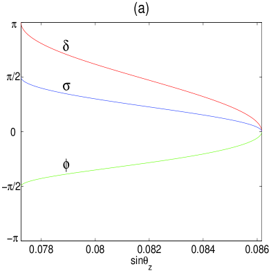
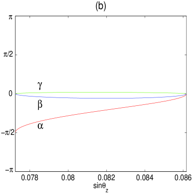
Figure 4.1: Numerical results for the FGY ansatz with $m_{1}=0$: (a) dependence of $\delta$, $\sigma$ and $\phi$ on $\sin\theta_{z}$; (b) dependence of $\alpha$, $\beta$ and $\gamma$ on $\sin\theta_{z}$.

Finally let us take a look at another two-zero texture of $M_{\rm D}$, in which $a_{2}=0$ and $b_{1}=0$ hold. The resultant neutrino mass matrix $M_{\nu}$ has a vanishing entry: $(M_{\nu})_{12}=0$. In this case, one may choose $a_{3}$ to be complex. The relevant phase parameters can then be calculated by setting $(M_{\nu})_{12}=0$ in Eq. (4.9). We find that the simple replacements $\delta\rightarrow\delta-\pi$ and $\theta_{y}\rightarrow\pi/2-\theta_{y}$ allow us to directly write out the expressions of $\sigma$, $\phi$, $\alpha$, $\beta$ and $\gamma$ in the $(M_{\nu})_{12}=0$ case from Eqs. (4.10), (4.11) and (4.12). It turns out that the numerical results of $\sigma$, $\phi$ and $\alpha$ are essentially unchanged, but those of $\beta$, $\gamma$ and $J_{\rm CP}$ require the replacements $\beta\leftrightarrow\gamma$ and $J_{\rm CP}\rightarrow-J_{\rm CP}$.

4.3 More Texture Zeros

It is straightforward to consider more texture zeros in $M_{\rm D}$. If $n$ (for $n=1,2,\cdots,6$) elements of $M_{\rm D}$ are vanishing, there are totally

$${\bf C}^{n}_{6}=\frac{6!}{n!(6-n)!}$$ (4.13)

patterns of $M_{\rm D}$. In the case of $n=3$, we are left with $20$ distinct textures of $M_{\rm D}$:

$${\rm Patterns~{}A1~{}to~{}A4} : ~{}~{}\left(\begin{matrix}{\bf 0}&{\bf 0}\cr{\bf 0}&\times\cr\times&\times\cr\end{matrix}\right)\;,~{}\left(\begin{matrix}{\bf 0}&{\bf 0}\cr\times&{\bf 0}\cr\times&\times\cr\end{matrix}\right)\;,~{}\left(\begin{matrix}{\bf 0}&{\bf 0}\cr\times&\times\cr{\bf 0}&\times\cr\end{matrix}\right)\;,~{}\left(\begin{matrix}{\bf 0}&{\bf 0}\cr\times&\times\cr\times&{\bf 0}\cr\end{matrix}\right)\;;~{}~{}~{}~{}~{}~{}~{}~{}$$ (4.14)

$${\rm Patterns~{}B1~{}to~{}B4} : ~{}~{}\left(\begin{matrix}{\bf 0}&\times\cr{\bf 0}&{\bf 0}\cr\times&\times\cr\end{matrix}\right)\;,~{}\left(\begin{matrix}\times&{\bf 0}\cr{\bf 0}&{\bf 0}\cr\times&\times\cr\end{matrix}\right)\;,~{}\left(\begin{matrix}\times&\times\cr{\bf 0}&{\bf 0}\cr{\bf 0}&\times\cr\end{matrix}\right)\;,~{}\left(\begin{matrix}\times&\times\cr{\bf 0}&{\bf 0}\cr\times&{\bf 0}\cr\end{matrix}\right)\;;~{}~{}~{}~{}~{}~{}~{}~{}$$ (4.15)

$${\rm Patterns~{}C1~{}to~{}C4} : ~{}~{}\left(\begin{matrix}{\bf 0}&\times\cr\times&\times\cr{\bf 0}&{\bf 0}\cr\end{matrix}\right)\;,~{}\left(\begin{matrix}\times&{\bf 0}\cr\times&\times\cr{\bf 0}&{\bf 0}\cr\end{matrix}\right)\;,~{}\left(\begin{matrix}\times&\times\cr{\bf 0}&\times\cr{\bf 0}&{\bf 0}\cr\end{matrix}\right)\;,~{}\left(\begin{matrix}\times&\times\cr\times&{\bf 0}\cr{\bf 0}&{\bf 0}\cr\end{matrix}\right)\;;~{}~{}~{}~{}~{}~{}~{}~{}$$ (4.16)

$${\rm Patterns~{}D1~{}to~{}D4} : ~{}~{}\left(\begin{matrix}{\bf 0}&\times\cr{\bf 0}&\times\cr{\bf 0}&\times\cr\end{matrix}\right)\;,~{}\left(\begin{matrix}\times&{\bf 0}\cr{\bf 0}&\times\cr{\bf 0}&\times\cr\end{matrix}\right)\;,~{}\left(\begin{matrix}{\bf 0}&\times\cr\times&{\bf 0}\cr{\bf 0}&\times\cr\end{matrix}\right)\;,~{}\left(\begin{matrix}{\bf 0}&\times\cr{\bf 0}&\times\cr\times&{\bf 0}\cr\end{matrix}\right)\;;~{}~{}~{}~{}~{}~{}~{}~{}$$ (4.17)

$${\rm Patterns~{}E1~{}to~{}E4} : ~{}~{}~{}\left(\begin{matrix}\times&{\bf 0}\cr\times&{\bf 0}\cr\times&{\bf 0}\cr\end{matrix}\right)\;,~{}\left(\begin{matrix}{\bf 0}&\times\cr\times&{\bf 0}\cr\times&{\bf 0}\cr\end{matrix}\right)\;,~{}\left(\begin{matrix}\times&{\bf 0}\cr{\bf 0}&\times\cr\times&{\bf 0}\cr\end{matrix}\right)\;,~{}\left(\begin{matrix}\times&{\bf 0}\cr\times&{\bf 0}\cr{\bf 0}&\times\cr\end{matrix}\right)\;,~{}~{}~{}~{}~{}~{}~{}~{}~{}$$ (4.18)

in which “$\times$” denotes an arbitrary non-vanishing matrix element.

It is quite obvious that the textures of $M_{\nu}$ resulting from Category A, B or C of $M_{\rm D}$ have been ruled out by current experimental data, because they only have non-vanishing entries in the (2,3), (3,1) or (1,2) block and cannot give rise to the phenomenologically-favored bi-large neutrino mixing pattern. Categories D and E of $M_{\rm D}$ can be transformed into each other by the exchange between $a_{i}$ and $b_{i}$ (for $i=1,2,3$). Hence let us examine the four patterns of $M_{\rm D}$ in Category D. Given three (or more) texture zeros in $M_{\rm D}$, its non-vanishing elements can all be chosen to be real by redefining the phases of three charged lepton fields. Considering Pattern D1, for example, we have

$$M_{\nu}=\frac{1}{M_{2}}\left(\begin{matrix}b^{2}_{1}&~{}~{}b_{1}b_{2}~{}~{}&b_{1}b_{3}\cr b_{2}b_{1}&b^{2}_{2}&b_{2}b_{3}\cr b_{3}b_{1}&b_{3}b_{2}&b^{2}_{3}\cr\end{matrix}\right)\;,$$ (4.19)

which is actually of rank one and has two vanishing neutrino mass eigenvalues. This result does conflict with the neutrino oscillation data. As for Patterns D2, D3 and D4, the resultant textures of $M_{\nu}$ are

$$~{}~{}~{}~{}~{}~{}~{}\left(\begin{matrix}\times&{\bf 0}&{\bf 0}\cr{\bf 0}&\times&\times\cr{\bf 0}&\times&\times\cr\end{matrix}\right)\;,~{}~{}~{}~{}\left(\begin{matrix}\times&{\bf 0}&\times\cr{\bf 0}&\times&{\bf 0}\cr\times&{\bf 0}&\times\cr\end{matrix}\right)\;,~{}~{}~{}~{}\left(\begin{matrix}\times&\times&{\bf 0}\cr\times&\times&{\bf 0}\cr{\bf 0}&{\bf 0}&\times\cr\end{matrix}\right)\;,$$ (4.20)

respectively. These three two-zero textures of $M_{\nu}$ have also been excluded by the present experimental data.[17, 37] Therefore, we conclude that the patterns of $M_{\rm D}$ with three or more texture zeros are all phenomenologically disfavored in the MSM.

4.4 Radiative Corrections

Now we discuss the possible renormalization-group running effects on neutrino masses and lepton flavor mixing parameters between the electroweak scale and the seesaw scale in the MSM. At energies far below the mass of the lighter right-handed Majorana neutrino $M_{1}$, two right-handed Majorana neutrino fields can be integrated out from the theory. Such a treatment will induce a dimension-5 operator $\overline{l_{\rm L}}\tilde{H}\kappa\tilde{H}^{T}l^{c}_{\rm L}$ in the effective Lagrangian, whose coupling matrix takes the canonical seesaw form at the scale $\mu=M_{1}$:

$$\kappa^{~{}}(M_{1})\;=\;-Y^{~{}}_{\nu}M^{-1}_{\rm R}Y^{\rm T}_{\nu}\;.$$ (4.21)

After the spontaneous gauge symmetry breaking, one may obtain the effective mass matrix of three light (left-handed) Majorana neutrinos $M_{\nu}=v^{2}\kappa(M_{Z})$ at the electroweak scale $\mu=M_{Z}$.

In the flavor basis where the charged-lepton and right-handed Majorana neutrino mass matrices are both diagonal, one can simplify the one-loop renormalization-group equations (RGEs).[46, 47] The effective coupling matrix $\kappa$ will receive radiative corrections when the energy scale runs from $M_{1}$ down to $M_{Z}$. To be more explicit, $\kappa(M_{Z})$ and $\kappa(M_{1})$ can be related to each other via

$$\kappa(M_{Z})\;=\;I_{\alpha}\left(\begin{matrix}I_{e}&0&0\cr 0&I_{\mu}&0\cr 0&0&I_{\tau}\cr\end{matrix}\right)\kappa(M_{1})\left(\begin{matrix}I_{e}&0&0\cr 0&I_{\mu}&0\cr 0&0&I_{\tau}\cr\end{matrix}\right)\;,$$ (4.22)

where $I_{\alpha}$ and $I_{l}$ ( for $l=e,\mu,\tau$ ) are the RGE evolution functions.[47] The overall factor $I_{\alpha}$ only affects the magnitudes of light neutrino masses, while $I^{~{}}_{l}$ can modify the neutrino masses, flavor mixing angles and CP-violating phases.[48] The strong mass hierarchy of three charged leptons (i.e., $m_{e}<m_{\mu}<m_{\tau}$) implies that $I_{e}<I_{\mu}<I_{\tau}$ holds below the scale $\mu=M_{1}$.[47] Two comments are in order.

1. The determinant of $\kappa$, which vanishes at $\mu=M_{1}$, keeps vanishing at $\mu=M_{Z}$. This point can clearly be seen from the relation

   $${\rm Det}[\kappa(M_{Z})]\;=\;I^{3}_{\alpha}I^{2}_{e}I^{2}_{\mu}I^{2}_{\tau}~{}{\rm Det}[\kappa(M_{1})]\;.$$ (4.23)

   Taking account of $m_{1}=0$ or $m_{3}=0$, we have $\left|{\rm Det}[\kappa(M_{Z})]\right|=m_{1}m_{2}m_{3}/v^{6}=0$.

2. Comparing between Eqs. (4.21) and (4.22), we find that the radiative correction to $\kappa$ can effectively be expressed as the RGE running effects in the elements of $M_{\rm D}$ (i.e., $a_{i}$ and $b_{i}$):

   $$a_{1}(M_{Z}) = I_{e}\sqrt{I_{\alpha}}~{}a_{1}(M_{1})\;,$$

   $$a_{2}(M_{Z}) = I_{\mu}\sqrt{I_{\alpha}}~{}a_{2}(M_{1})\;,$$

   $$a_{3}(M_{Z}) = I_{\tau}\sqrt{I_{\alpha}}~{}a_{3}(M_{1})\;,$$ (4.24)

   with the assumption that $M_{1}$ keeps unchanged. The same relations can be obtained for $b_{i}$ (for $i=1,2,3$) at two different energy scales. This observation indicates that possible texture zeros of $\kappa$ at $\mu=M_{1}$ remain there even at $\mu=M_{Z}$, at least at the one-loop level of the RGE evolution. In other words, the texture zeros of $\kappa$ are essentially stable against quantum corrections from $M_{1}$ to $M_{Z}$.

To illustrate, we typically take the top-quark mass $m_{t}(M_{Z})\approx 181~{}{\rm GeV}$ to calculate the evolution functions $I_{\alpha}$ and $I^{~{}}_{l}$ (for $l=e,\mu,\tau$). It turns out that $I_{e}\approx I_{\mu}\approx 1$ is an excellent approximation in the SM. Thus the RGE running of $\kappa$ is mainly governed by $I_{\alpha}$ and $I_{\tau}$. The behaviors of $I_{\alpha}$ and $I_{\tau}$ changing with $M_{1}$ are shown in Fig. 4.2. One can see that $I_{\tau}\approx 1$ is also a good approximation in the SM and in the MSSM with mild values of $\tan\beta$. Hence the evolution of three light neutrino masses are dominated by $I_{\alpha}$, which may significantly deviate from unity.

file=fig4.2.eps,bbllx=2cm,bblly=2cm,bburx=21cm,bbury=24cm, width=14.0cm,height=15cm,angle=0,clip=0

Figure 4.2: Numerical illustration of the evolution functions $I_{\alpha}$ and $I_{\tau}$ changing with $M_{1}$ for different values of the Higgs mass $m^{~{}}_{H}$ in the SM (up) or for different values of $\tan\beta$ in the MSSM (down).

We proceed to discuss radiative corrections to three neutrino masses. For simplicity, here we mainly consider the $m_{1}=0$ case. The RGE running of $m_{i}$, $\dot{m}_{i}\equiv{\rm d}m_{i}/{\rm d}t$ with $t=[\ln(\mu/M_{Z})]/(16\pi^{2})$, is proportional to $m_{i}$ itself (for $i=1,2,3$) at the one-loop level.[46] Explicitly,[47]

$$\dot{m}_{1} = 0\;,$$

$$\dot{m}_{2} \approx \frac{1}{16\pi^{2}}\left(\alpha+2Cf_{\tau}^{2}c_{x}^{2}s_{y}^{2}\right)m_{2}\;,$$

$$\dot{m}_{3} \approx \frac{1}{16\pi^{2}}\left(\alpha+2Cf_{\tau}^{2}c_{y}^{2}\right)m_{3}\;,$$ (4.25)

where $C=-3/2$ (SM) or 1 (MSSM), $\alpha$ denotes the contribution from both the gauge couplings and the top-quark Yukawa coupling,[46] and $f_{\tau}$ is the tau-lepton Yukawa coupling. It becomes clear that the running behaviors of $m_{2}$ and $m_{3}$ are essentially identical.[47] For illustration, we show the ratio ${\rm R}\equiv m_{2}(M_{Z})/m_{2}(M_{1})$ changing with the Higgs mass $m^{~{}}_{H}$ (SM) or with $\tan\beta$ (MSSM) in Fig. 4.3, where $M_{1}=10^{14}$ GeV has typically been taken and the $m_{3}=0$ case is also included. One can see that ${\rm R}_{m_{1}=0}\approx{\rm R}_{m_{3}=0}\approx I_{\alpha}$ is an excellent approximation in the SM or in the MSSM with mild values of $\tan\beta$.

file=fig4.3.eps,bbllx=2cm,bblly=2cm,bburx=21cm,bbury=24cm, width=14.0cm,height=15cm,angle=0,clip=0

Figure 4.3: Numerical illustration of the ratio $R\equiv m_{2}(M_{Z})/m_{2}(M_{1})$ as a function of $m_{H}$ in the SM (up) or of $\tan\beta$ in the MSSM (down), where $M_{1}=10^{14}$ GeV has typically been input for the MSM with either $m_{1}=0$ or $m_{3}=0$.

The RGEs of three flavor mixing angles $(\theta_{x},\theta_{y},\theta_{z})$ and two CP-violating phases $(\delta,\sigma)$ in the $m_{1}=0$ case are approximately given by[47]

$$\dot{\theta}_{x} \approx -\frac{Cf_{\tau}^{2}}{16\pi^{2}}s_{x}c_{x}s_{y}^{2}\;,$$

$$\dot{\theta}_{y} \approx -\frac{Cf_{\tau}^{2}}{16\pi^{2}}s_{y}c_{y}\left(1+2r_{23}c_{x}^{2}\cos\delta\right)\;,$$

$$\dot{\theta}_{z} \approx -\frac{Cf_{\tau}^{2}}{8\pi^{2}}r_{23}s_{x}c_{x}s_{y}c_{y}\;;$$ (4.26)

and

$$\dot{\sigma} \approx \frac{Cf_{\tau}^{2}}{8\pi^{2}}\left(s_{x}c_{x}s_{y}c_{y}\frac{r_{23}}{s_{z}}\right)r_{23}\sin\delta\;,$$

$$\dot{\delta} \approx \frac{Cf_{\tau}^{2}}{8\pi^{2}}\left[s_{x}c_{x}s_{y}c_{y}\frac{r_{23}}{s_{z}}+c^{2}_{x}\left(c_{y}^{2}-s_{y}^{2}\right)\right]r_{23}\sin\delta\;,$$ (4.27)

where $r_{23}\equiv m_{2}/m_{3}$ has been defined before. We see that the running effects of these five parameters are all governed by $f^{2}_{\tau}$. Because of $f^{2}_{\tau}\approx 10^{-4}$ in the SM, the evolution of $(\theta_{x},\theta_{y},\theta_{z})$ and $(\sigma,\delta)$ is negligibly small. When $\tan\beta$ is sufficiently large (e.g., $\tan\beta\sim 50$) in the MSSM, however, $f^{2}_{\tau}\approx 10^{-4}/\cos^{2}\beta$ can be of ${\cal O}(0.1)$ and even close to unity — in this case, some small variation of $(\theta_{x},\theta_{y},\theta_{z})$ and $(\sigma,\delta)$ due to the RGE running from $M_{Z}$ to $M_{1}$ will appear. A detailed analysis[47] has shown that the smallest neutrino mixing angle $\theta_{z}$ is most sensitive to radiative corrections, but its change from $\mu=M_{Z}$ to $\mu=M_{1}$ is less than $10\%$ even if $M_{1}=10^{14}$ GeV and $\tan\beta=50$ are taken. Thus we conclude that the RGE effects on three flavor mixing angles and two CP-violating phases are practically negligible in the MSM with $m_{1}=0$. As for the $m_{3}=0$ case, it is found that the near degeneracy between $m_{1}$ and $m_{2}$ may result in significant RGE running effects on the mixing angle $\theta_{x}$ in the MSSM, and the evolution of two CP-violating phases can also be appreciable if both $M_{1}$ and $\tan\beta$ take sufficiently large values.[47]

4.5 Non-Diagonal $M_{l}$ and $M_{\rm R}$

So far we have been working in the flavor basis where both $M_{l}$ and $M_{\rm R}$ are diagonal. In an arbitrary flavor basis, however, $M_{l}$ and $M_{\rm R}$ need to be diagonalized by using proper unitary transformations:

$$M_{l}\;=\;U_{l}\left(\begin{matrix}m_{e}&0&0\cr 0&m_{\mu}&0\cr 0&0&m_{\tau}\cr\end{matrix}\right)\tilde{U}^{\dagger}_{l}\;,$$ (4.28)

and

$$M_{\rm R}\;=\;U_{\rm R}\left(\begin{matrix}M_{1}~{}&~{}0\cr 0~{}&~{}M_{2}\cr\end{matrix}\right)U^{T}_{\rm R}\;.$$ (4.29)

When $M_{l}$ is Hermitian or symmetric, we have $\tilde{U}_{l}=U_{l}$ or $\tilde{U}_{l}=U^{*}_{l}$. The MNS matrix is in general given by $V_{\rm MNS}=U^{\dagger}_{l}V$, where $V$ is the unitary matrix used to diagonalize the effective neutrino mass matrix $M_{\nu}$ in Eq. (2.6). Without loss of generality, $U_{l}$ can be parameterized in terms of three rotation angles and one phase, while $U_{\rm R}$ can be parameterized in terms of one rotation angle and one phase.

Let us make some brief comments on the texture of $M_{\rm D}$ in the flavor basis where $M_{l}$ and $M_{\rm R}$ are not diagonal. There are two possibilities:

1. $M_{\rm D}$ has no texture zeros. By redefining the fields $l_{\rm L}$, $E_{\rm R}$ and $N_{\rm R}$, we transform $M_{l}$ and $M_{\rm R}$ into the diagonal mass matrices $\tilde{M}_{l}$ and $\tilde{M}_{\rm R}$. Then $M_{\rm D}$ becomes $\tilde{M}_{\rm D}=U_{l}^{\dagger}M_{\rm D}U_{\rm R}^{*}$ in the new basis. If $\tilde{M}_{\rm D}$ has no texture zeros, we cannot get any extra constraint on the seesaw relation. Provided $\tilde{M}_{\rm D}$ has texture zeros, $(\tilde{M}_{\rm D})_{ij}=0$, then we have

   $$(\tilde{M}_{\rm D})_{ij}\;=\left(iV_{\rm MNS}\sqrt{m}R\sqrt{M^{\prime}_{\rm R}}\right)_{ij}=0\;$$ (4.30)

   in the Casas-Ibarra-Ross parameterization, where $\sqrt{M^{\prime}_{\rm R}}=R^{\prime}\sqrt{M_{\rm R}}U^{*}_{\rm R}$ is a diagonal matrix with $R^{\prime}$ being a $2\times 2$ orthogonal matrix.

2. $M_{\rm D}$ has texture zeros. Then $(M_{\rm D})_{ij}=0$ means

   $$(M_{\rm D})_{ij}\;=\;\left(iU_{l}V_{\rm MNS}\sqrt{m}R\sqrt{M_{\rm R}}\right)_{ij}=0$$ (4.31)

   in the Casas-Ibarra-Ross parameterization. After transforming $M_{l}$ and $M_{\rm R}$ into $\tilde{M}_{l}$ and $\tilde{M}_{\rm R}$, we get $\tilde{M}_{\rm D}=U_{l}^{\dagger}M_{\rm D}U_{\rm R}^{*}$ in the new basis. If $\tilde{M}_{\rm D}$ has texture zeros, Eq. (4.30) will be applicable. Otherwise, only Eq. (4.31) can impose some constraints on the model.[23, 40]

4.6 Comments on Model Building

To dynamically understand possible texture zeros in $M_{\rm D}$, one may incorporate a certain flavor symmetry in the supersymmetric version of the MSM. For illustration, we first consider the $SU(2)_{\rm H}$ horizontal symmetry. In the presence of a local $SU(2)_{\rm H}$ horizontal symmetry under which right-handed charged leptons transform nontrivially, freedom from global anomalies requires that there be at least two right-handed neutrinos with masses of order of the horizontal symmetry breaking scale.[40] Taking account of the quark-lepton symmetry, one may introduce an extra right-handed neutrino, which is the $SU(2)_{\rm H}$ singlet and too heavy to couple to low-energy physics. In the leptonic sector, the $SU(2)_{\rm H}$ doublets include $(l_{e\rm L},l_{\mu\rm L})$, $(\mu_{\rm R},-e_{\rm R})$ and $(\nu_{\mu\rm R},-\nu_{e\rm R})$, and the $SU(2)_{\rm H}$ singlets are $l_{\tau\rm L}$, $\tau_{\rm R}$ and $\nu_{\tau\rm R}$. In addition to the MSSM Higgs doublets $H_{1}$ and $H_{2}$, the new Higgs doublets $\chi=(\chi_{1},\chi_{2})$ and $\bar{\chi}=(-\bar{\chi}_{2},\bar{\chi}_{1})$ are assumed. The gauge-invariant Yukawa couplings relevant for the Dirac neutrino mass matrix is given by[40]

$$W_{\rm Y}=h_{0}\left(l_{e\rm L}H_{2}\nu_{e\rm R}+l_{\mu\rm L}H_{2}\nu_{\mu\rm R}\right)+h_{1}l_{\tau\rm L}\left(\nu_{\mu\rm R}\chi_{2}+\nu_{e\rm R}\chi_{1}\right)H_{2}/M\;,$$ (4.32)

where $M$ can be regarded as the scale of the horizontal symmetry breaking. After the horizontal and gauge symmetries are spontaneously broken down, the Higgs fields gain their vevs as $\langle H_{i}\rangle=v_{i}$, $\langle\chi_{i}\rangle=u_{i}$ (for $i=1,2$). Then we obtain the Dirac neutrino mass matrix

$$M_{\rm D}=\left(\begin{matrix}h_{0}v_{2}&{\bf 0}\cr{\bf 0}&h_{0}v_{2}\cr h_{1}w_{1}&h_{1}w_{2}\cr\end{matrix}\right)\;,$$ (4.33)

where $w_{i}\equiv v_{2}u_{i}/M$ (for $i=1,2$). Note that the mass matrices $M_{l}$ and $M_{\rm R}$ are in general not diagonal. This scenario indicates that the MSM can be viewed as the special case of a more generic seesaw model with three right-handed Majorana neutrinos, when one of them is so heavy that it essentially decouples from low-energy physics.

Another simple scenario, in which the MSM is incorporated with a $SU(2)\times U(1)$ family symmetry, has also been proposed.[39] It can naturally result in the texture of $M_{\rm D}$ in Eq. (4.5). The superpotential relevant for $M_{\rm D}$ in this model is written as[39]

$$W_{\rm Y}=\frac{H}{M}\left(L_{a}\phi^{a}N_{1}+L_{a}\tilde{\phi}^{a}N_{2}+l_{3}\omega N_{2}\right)+\frac{1}{2}\left(S^{~{}}_{1}N_{1}^{2}+S^{~{}}_{2}N_{2}^{2}\right)\;,$$ (4.34)

where $L_{a}=(l_{\rm L1},~{}l_{\rm L2})^{T}$ is a doublet of the $SU(2)$ family symmetry, while $l_{\rm L3}$ is a singlet. In addition, two flavor (anti)-doublets ($\phi^{a}$ and $\tilde{\phi}^{a}$), four flavor singlets ($N_{1}$, $N_{2}$, $S_{1}$ and $S_{2}$) and the SM Higgs doublet $H$ are introduced. Note that $M$ is a superhigh mass scale in Eq. (4.34). In the basis where $M_{l}$ is diagonal, the $U(1)$ charge assignments for the fields $\{L_{a},l_{3},N_{1},N_{2},\phi^{a},\tilde{\phi}^{a},\omega,S_{1},\ S_{2}\}$ are $\{1,\xi,x,y,-(x+1),-(y+1),-(\xi+y),-2x,-2y\}$ with $x\neq y$. We assume that $\phi$ and $\tilde{\phi}$ can get vevs $\langle\phi\rangle=(\phi^{1},~{}\phi^{2})^{T}$ and $\langle\tilde{\phi}\rangle=(0,~{}\tilde{\phi}^{2})^{T}$. The vevs $\langle S_{i}\rangle=M_{i}$ (for $i=1,2$) are also needed to give the states $N_{i}$ sufficiently large masses. These vevs can be obtained via the suitable terms added to the above superpotential.[39] Then we obtain the texture of $M_{\rm D}$ as given in Eq. (4.5), where

$$a_{1} = v\sin\beta\frac{\phi^{1}}{\sqrt{2}M}\;,$$

$$a_{2} = v\sin\beta\frac{\phi^{2}}{\sqrt{2}M}\;,$$

$$b_{2} = v\sin\beta\frac{\tilde{\phi}^{2}}{\sqrt{2}M}\;,$$

$$b_{3} = v\sin\beta\frac{\omega}{\sqrt{2}M}\;,$$ (4.35)

together with $\langle H\rangle=(0,~{}v\sin\beta)^{T}$. These vevs are in general complex.

Finally, it is worth mentioning that the FGY ansatz can also be derived from certain extra-dimensional models.[35] Another possibility to obtain the texture zeros in $M_{\rm D}$ is to require the vanishing of certain CP-odd invariants together with a reasonable assumption of no conspiracy among the parameters of $M_{\rm D}$ and $M_{\rm R}$.[42]

5 Baryogenesis via Leptogenesis

The cosmological baryon number asymmetry is one of the most striking mysteries in the Universe. Thanks to the three-year WMAP observation,[49] the ratio of baryon to photon number densities can now be determined to a very good precision: $\eta_{\rm B}\equiv n^{~{}}_{\rm B}/n^{~{}}_{\gamma}=(6.1\pm 0.2)\times 10^{-10}$. This tiny quantity measures the observed matter-antimatter or baryon-antibaryon asymmetry of the Universe,

$$Y_{\rm B}\;\equiv\;\frac{n^{~{}}_{\rm B}-n^{~{}}_{\rm\bar{B}}}{\bf s}\;\approx\;\frac{\eta_{\rm B}}{7.04}\;\approx\;(8.66\pm 0.28)\times 10^{-11}\;,$$ (5.1)

where $\bf s$ denotes the entropy density. To dynamically produce a net baryon number asymmetry in the framework of the standard Big-Bang cosmology, three Sakharov necessary conditions have to be satisfied:[7] (a) baryon number non-conservation, (b) C and CP violation, and (c) departure from thermal equilibrium. Among a number of baryogenesis mechanisms existing in the literature,[50] the one via leptogenesis[8] is particularly interesting and closely related to neutrino physics.

5.1 Thermal Leptogenesis

First of all, let us outline the main points of thermal leptogenesis in the MSM. The decays of two heavy right-handed Majorana neutrinos, $N_{i}\rightarrow l+H^{\dagger}$ and $N_{i}\rightarrow l^{c}+H$ (for $i=1,2$), are both lepton-number-violating and CP-violating. The CP asymmetry $\varepsilon_{i}$ arises from the interference between the tree-level and one-loop decay amplitudes. If $N_{1}$ and $N_{2}$ have a hierarchical mass spectrum ($M_{1}\ll M_{2}$), the interactions involving $N_{1}$ can be in thermal equilibrium when $N_{2}$ decays. Hence $\varepsilon_{2}$ is erased before $N_{1}$ decays. The CP-violating asymmetry $\varepsilon_{1}$, which is produced by the out-of-equilibrium decay of $N_{1}$, may finally survive. For simplicity, we assume $M_{1}\ll M_{2}$ here and in Sec. 5.2. The possibility of $M_{1}\approx M_{2}$, which gives rise to the resonant leptogenesis,[51] will be discussed in Sec. 5.3.

In the flavor basis where the mass matrices of charged leptons ($M_{l}$) and right-handed Majorana neutrinos ($M_{\rm R}$) are both diagonal, one may calculate the CP-violating asymmetry $\varepsilon_{1}$:[52]

$$\varepsilon_{1} \equiv \frac{\Gamma(N_{1}\rightarrow l+H^{\dagger})-\Gamma(N_{1}\rightarrow l^{\rm c}+H)}{\Gamma(N_{1}\rightarrow l+H^{\dagger})+\Gamma(N_{1}\rightarrow l^{\rm c}+H)}$$ (5.2)

$$\approx -\frac{3}{16\pi v^{2}}\frac{M_{1}}{M_{2}}\frac{{\rm Im}\left[(M^{\dagger}_{\rm D}M^{~{}}_{\rm D})^{2}_{12}\right]}{(M^{\dagger}_{\rm D}M^{~{}}_{\rm D})_{11}}\;.$$ (5.3)

Leptogenesis means that $\varepsilon_{1}$ gives rise to a net lepton number asymmetry in the Universe,

$$Y_{\rm L}\equiv\frac{n_{\rm L}-n_{\bar{{\rm L}}}}{\bf s}=\frac{\kappa}{g_{*}}\;\varepsilon_{1}\;,$$ (5.4)

where $g_{*}=106.75$ is an effective number characterizing the relativistic degrees of freedom which contribute to the entropy of the early Universe, and $\kappa$ accounts for the dilution effects induced by the lepton-number-violating wash-out processes. The efficiency factor $\kappa$ can be figured out by solving the full Boltzmann equations.[52] For simplicity, here we take the following analytical approximation for $\kappa$:[54]

$$\kappa\;\approx\;0.3\left(\frac{10^{-3}~{}{\rm eV}}{\tilde{m}_{1}}\right)\left[\ln\left(\frac{\tilde{m}_{1}}{10^{-3}~{}{\rm eV}}\right)\right]^{-0.6}\;$$ (5.5)

with $\tilde{m}_{1}=(M^{\dagger}_{\rm D}M_{\rm D})_{11}/{M_{1}}$. The lepton number asymmetry $Y_{\rm L}$ is eventually converted into a net baryon number asymmetry $Y_{\rm B}$ via the non-perturbative sphaleron processes,[9, 55]

$$Y_{\rm B}=-c\;Y_{\rm L}\;,$$ (5.6)

where $c=28/79\approx 0.35$ in the SM. A similar relation between $Y_{\rm B}$ and $Y_{\rm L}$ can be obtained in the supersymmetric extension of the MSM.[52]

5.2 Upper Bound of $|\varepsilon_{1}|$

In those seesaw models with three right-handed Majorana neutrinos, the CP-violating asymmetry $\varepsilon_{1}$ has an upper bound[56]

$$|\varepsilon_{1}| \leq \frac{3M_{1}}{16\pi v^{2}}\left|\frac{m_{2}^{2}-m_{1}^{2}}{m_{2}}+\frac{m_{3}^{2}-m_{1}^{2}}{m_{3}}\right|\;.$$ (5.7)

Since $m_{1}$ or $m_{3}$ must be massless in the MSM, we ought to obtain more rigorous constraints on $|\varepsilon_{1}|$.[23] But it is not proper to directly substitute $m_{1}=0$ or $m_{3}=0$ into Eq. (5.6). With the help of Eqs. (2.4) and (2.6), the expression of $\varepsilon_{1}$ in Eq. (5.2) can be rewritten as

$$\varepsilon_{1} \approx -\frac{3}{16\pi v^{2}}\frac{M_{1}}{(M^{\dagger}_{\rm D}M_{\rm D})_{11}}{\rm Im}\left[(M^{T}_{\rm D}M^{*}_{\nu}M_{\rm D})_{11}\right],\;$$ (5.8)

$$\approx -\frac{3}{16\pi v^{2}}\frac{M_{1}}{(M^{\dagger}_{\rm D}M_{\rm D})_{11}}{\rm Im}\left\{\left[(V^{\dagger}M_{\rm D})^{T}m(V^{\dagger}M_{\rm D})\right]_{11}\right\}\;,$$ (5.9)

where $m\equiv{\rm Diag}\{m_{1},m_{2},m_{3}\}$ with either $m_{1}=0$ or $m_{3}=0$, and $V$ is the MNS matrix. In the $m_{1}=0$ case, we adopt the Casas-Ibarra-Ross parametrization of $M_{\rm D}$ and define

$$K\equiv V^{\dagger}M_{\rm D}=i\sqrt{m}~{}R\sqrt{M_{\rm R}}\;\;.$$ (5.10)

Because of $K_{1i}=0$, we obtain $(M^{\dagger}_{\rm D}M^{~{}}_{\rm D})_{11}=(K^{\dagger}K)_{11}=|K_{21}|^{2}+|K_{31}|^{2}$. In addition,

$${\rm Im}\left\{\left[(V^{\dagger}M_{\rm D})^{T}m(V^{\dagger}M_{\rm D})\right]_{11}\right\} = {\rm Im}\left[(K^{T}mK)_{11}\right]$$ (5.11)

$$= m_{2}{\rm Im}\left[K^{2}_{21}\right]+m_{3}{\rm Im}\left[K^{2}_{31}\right]\;$$

and $m_{2}{\rm Im}[K^{2}_{31}]+m_{3}{\rm Im}[K^{2}_{21}]=0$ hold.[23] Then $\varepsilon_{1}$ in Eq. (5.7) can be expressed as

$$\varepsilon_{1} \approx -\frac{3M_{1}}{16\pi v^{2}}\frac{m^{2}_{3}-m^{2}_{2}}{m_{3}}\frac{{\rm Im}[K^{2}_{31}]}{|K_{21}|^{2}+|K_{31}|^{2}}\;.$$ (5.12)

The upper bound of $|\varepsilon_{1}|$ turns out to be

$$|\varepsilon_{1}| \leq \frac{3M_{1}}{16\pi v^{2}}\frac{\Delta m^{2}_{\rm atm}}{\sqrt{\Delta m^{2}_{\rm atm}+\Delta m^{2}_{\rm sun}}}\;$$ (5.13)

in the $m_{1}=0$ case. Similarly, one may get

$$|\varepsilon_{1}| \leq \frac{3M_{1}}{16\pi v^{2}}\frac{\Delta m^{2}_{\rm sun}}{\sqrt{\Delta m^{2}_{\rm atm}}}\;~{}~{}~{}~{}~{}~{}~{}~{}~{}~{}~{}~{}$$ (5.14)

in the $m_{3}=0$ case.

In the MSM, the successful leptogenesis depends on three parameters: $\varepsilon_{1}$, $M_{1}$ and $\tilde{m}_{1}$. Because of the washout effects, which are characterized by $\tilde{m}_{1}$, the maximal $\varepsilon_{1}$ does not imply the minimal $M_{1}$. Taking $m_{1}=0$ for example and making use of Eqs. (3.2) and (5.8), we obtain

$$\frac{{\rm Im}[K^{2}_{31}]}{|K_{21}|^{2}+|K_{31}|^{2}}=-\frac{m_{3}{\rm Im}[\sin^{2}z]}{m_{2}|\cos z|^{2}+m_{3}|\sin z|^{2}}\;,$$ (5.15)

and

$$\tilde{m}_{1} = m_{2}|\cos z|^{2}+m_{3}|\sin z|^{2}\;.$$ (5.16)

These results indicate that $\tilde{m}_{1}\geq m_{2}$ holds. Furthermore,

$$m_{3}{\rm Im}[\sin^{2}z]\leq m_{3}|\sin z|^{2}=\tilde{m}_{1}-m_{2}|\cos z|^{2}\leq\tilde{m}_{1}-m_{2}\;.$$ (5.17)

With the help of Eqs. (5.10), (5.13), (5.14) and (5.15), we arrive at a new upper bound on $\varepsilon_{1}$:[23]

$$|\varepsilon_{1}| \leq \frac{3M_{1}}{16\pi v^{2}}\frac{\Delta m^{2}_{\rm atm}}{\sqrt{\Delta m^{2}_{\rm atm}+\Delta m^{2}_{\rm sun}}}\left(1-\frac{\sqrt{\Delta m^{2}_{\rm sun}}}{\tilde{m}_{1}}\right)\;,$$ (5.18)

in which the effect of $\tilde{m}_{1}$ has been taken into account. For the $m_{3}=0$ case, one may similarly obtain

$$|\varepsilon_{1}| \leq \frac{3M_{1}}{16\pi v^{2}}\frac{\Delta m^{2}_{\rm sun}}{\sqrt{\Delta m^{2}_{\rm atm}}}\left(1-\frac{\sqrt{\Delta m^{2}_{\rm atm}-\Delta m^{2}_{\rm sun}}}{\tilde{m}_{1}}\right)\;,$$ (5.19)

where $\tilde{m}_{1}$ satisfies $\tilde{m}_{1}\geq m_{1}$.

Using the maximal value of $\varepsilon_{1}$ in Eq. (5.16) or (5.17), together with the best-fit values of $\Delta m^{2}_{\rm sun}$ and $\Delta m^{2}_{\rm atm}$, we carry out a numerical analysis of $Y_{\rm B}$ versus $\tilde{m}_{1}$ and show the result in Fig. 5.1, where the observationally-allowed range of $Y_{\rm B}$ is taken to be $8.5\times 10^{-11}\leq Y_{\rm B}\leq 9.4\times 10^{-11}$. We see that the successful baryogenesis via leptogenesis requires $M_{1}\geq 5.9\times 10^{10}~{}{\rm GeV}$ in the $m_{1}=0$ case and $M_{1}\geq 1.3\times 10^{13}~{}{\rm GeV}$ in the $m_{3}=0$ case. Because $\tilde{m}_{1}\geq m_{2}$ holds for the normal neutrino mass hierarchy, we have

$$|a_{1}|^{2}+|a_{2}|^{2}+|a_{3}|^{2}\geq M_{1}m_{2}\geq 0.53~{}{\rm GeV}^{2}\;,$$ (5.20)

where $a_{i}$ (for $i=1,2,3$) are the matrix elements in the first column of $M_{\rm D}$. Thus the largest $|a_{i}|$ should not be smaller than $0.42~{}{\rm GeV}$. For the inverted neutrino mass hierarchy, we can similarly find that the largest $|a_{i}|$ should be above $14.6~{}{\rm GeV}$.

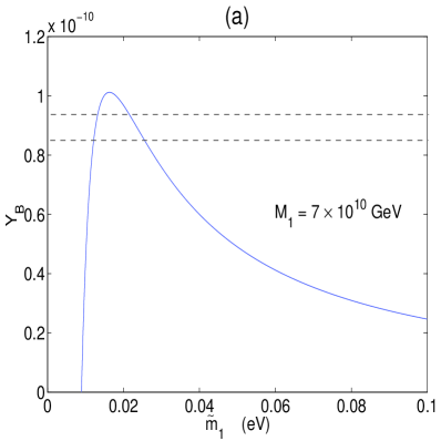
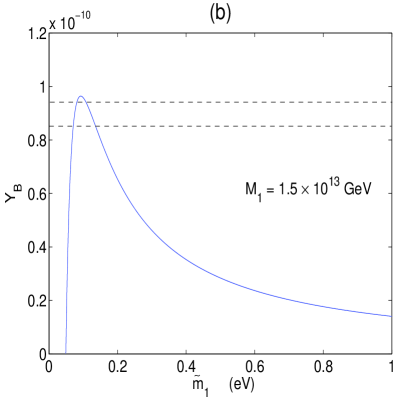
Figure 5.1: Numerical illustration of the correlation between $Y_{\rm B}$ and $\tilde{m}_{1}$ in the MSM: (a) the $m_{1}=0$ case; and (b) the $m_{3}=0$ case.

5.3 Resonant Leptogenesis

In the previous sections, we have discussed the simplest scenario of thermal leptogenesis with two hierarchical right-handed Majorana neutrinos. Another interesting scenario is the so-called resonant leptogenesis.[51] When the masses of two heavy Majorana neutrinos are approximately degenerate (i.e., $M_{1}\approx M_{2}$), the one-loop self-energy effect can be resonantly enhanced and play the dominant role in $\varepsilon_{1}$ and $\varepsilon_{2}$. It is then possible to generate the observed baryon number asymmetry $Y_{\rm B}$ through the out-of-equilibrium decays of relatively light and approximately degenerate $N_{1}$ and $N_{2}$. Such a scenario could allow us to relax the lower bound on the lighter right-handed Majorana neutrino mass $M_{1}$ in the MSM and to get clear of the gravitino overproduction problem in the supersymmetric version of the MSM.[57]

When the mass splitting between two heavy Majorana neutrinos is comparable to their decay widths, the CP-violating asymmetry $\varepsilon_{i}$ is dominated by the one-loop self-energy contribution[11]

$$\varepsilon_{i} = \frac{{\rm Im}\left[(M^{\dagger}_{\rm D}M^{~{}}_{\rm D})^{2}_{ij}\right]}{(M^{\dagger}_{\rm D}M^{~{}}_{\rm D})_{ii}(M^{\dagger}_{\rm D}M^{~{}}_{\rm D})_{jj}}\;\frac{(M^{2}_{i}-M^{2}_{j})\;M_{i}\;\Gamma_{j}}{(M^{2}_{i}-M^{2}_{j})^{2}+M^{2}_{i}\;\Gamma^{2}_{j}}\;,$$ (5.21)

where $\Gamma_{i}\equiv M_{i}\left(Y^{\dagger}_{\nu}Y_{\nu}\right)_{ii}/(8\pi)$ is the tree-level decay width of $N_{i}$. If $|M_{i}-M_{j}|\sim\Gamma_{i}/2$ holds, the factor $(M^{2}_{i}-M^{2}_{j})M_{i}\Gamma_{j}/[(M^{2}_{i}-M^{2}_{j})^{2}+M^{2}_{i}\Gamma^{2}_{j}]$ may approach its maximal value $1/2$. If the masses of two heavy Majorana neutrinos are exactly degenerate, however, $\varepsilon_{i}$ must vanish as one can see from Eq. (5.19).

A simple scenario of TeV-scale leptogenesis in the MSM has recently been proposed.[58] For simplicity, here let us concentrate on the $m_{1}=0$ case to introduce this phenomenological scenario. By using the bi-unitary parametrization, the $3\times 2$ Dirac neutrino mass matrix $M_{\rm D}$ can be expressed as

$$M_{\rm D}\;=\;V_{0}\left(\begin{matrix}0&0\cr x&0\cr 0&y\cr\end{matrix}\right)U\;,$$ (5.22)

where $V_{0}$ and $U$ are $3\times 3$ and $2\times 2$ unitary matrices, respectively. Then the seesaw relation $M_{\nu}=M_{\rm D}M^{-1}_{\rm R}M^{T}_{\rm D}$ implies that the flavor mixing of light neutrinos depends primarily on $V_{0}$ and the decays of heavy neutrinos rely mainly on $U$. This observation motivates us to take $V_{0}$ to be the tri-bimaximal mixing pattern[59]

$$V_{0}\;=\;\left(\begin{matrix}2/\sqrt{6}&1/\sqrt{3}&0\cr-1/\sqrt{6}&1/\sqrt{3}&1/\sqrt{2}\cr 1/\sqrt{6}&~{}~{}-1/\sqrt{3}~{}~{}&1/\sqrt{2}\cr\end{matrix}\right)\;,$$ (5.23)

which is compatible very well with the best fit of current experimental data on neutrino oscillations[15]. On the other hand, we assume $U$ to be the maximal mixing pattern with a single CP-violating phase,

$$U=\left(\begin{matrix}1/\sqrt{2}&1/\sqrt{2}\cr-1/\sqrt{2}&1/\sqrt{2}\cr\end{matrix}\right)\left(\begin{matrix}e^{-i\alpha}&0\cr 0&e^{+i\alpha}\cr\end{matrix}\right)\;.$$ (5.24)

Since $\alpha$ is the only phase parameter in our model, it should be responsible both for the CP violation in neutrino oscillations and for the CP violation in $N_{i}$ decays. In order to implement the idea of resonant leptogenesis, we assume that $N_{1}$ and $N_{2}$ are highly degenerate in mass; i.e., the magnitude of $r\equiv(M_{2}-M_{1})/M_{2}$ is strongly suppressed. Indeed $|r|\sim{\cal O}(10^{-7})$ or smaller has typically been anticipated in some seesaw models with three right-handed Majorana neutrinos[11] to gain the successful resonant leptogenesis.

Given $|r|<{\cal O}(10^{-4})$, the explicit form of $M_{\nu}$ can reliably be formulated from the seesaw relation $M_{\nu}=M_{\rm D}M^{-1}_{\rm R}M^{T}_{\rm D}$ by neglecting the tiny mass splitting between $N_{1}$ and $N_{2}$. In such a good approximation, we obtain

$$M_{\nu}\;=\;\frac{y^{2}}{M_{2}}\left[V_{0}\left(\begin{matrix}0&0&0\cr 0&\omega^{2}\cos 2\alpha&i\omega\sin 2\alpha\cr 0&i\omega\sin 2\alpha&\cos 2\alpha\cr\end{matrix}\right)V^{T}_{0}\right]\;,$$ (5.25)

where $\omega=x/y$. The diagonalization $V^{\dagger}M_{\nu}V^{*}={\rm Diag}\left\{0,m_{2},m_{3}\right\}$, where $V$ is just the MNS matrix, yields

$$m_{2} = \displaystyle\frac{y^{2}}{2M_{2}}\left[\sqrt{\left(1+\omega^{2}\right)^{2}\cos^{2}2\alpha+4\omega^{2}\sin^{2}2\alpha}~{}-\left(1-\omega^{2}\right)\left|\cos 2\alpha\right|\right]\;,$$

$$m_{3} = \displaystyle\frac{y^{2}}{2M_{2}}\left[\sqrt{\left(1+\omega^{2}\right)^{2}\cos^{2}2\alpha+4\omega^{2}\sin^{2}2\alpha}~{}+\left(1-\omega^{2}\right)\left|\cos 2\alpha\right|\right]\;,~{}~{}$$ (5.26)

where $0<\omega<1$. Taking account of $m_{2}=\sqrt{\Delta m^{2}_{21}}$ and $m_{3}=\sqrt{\Delta m^{2}_{21}+|\Delta m^{2}_{32}|}$, we obtain $m_{2}\approx 8.9\times 10^{-3}$ eV and $m_{3}\approx 5.1\times 10^{-2}$ eV by using $\Delta m^{2}_{21}\approx 8.0\times 10^{-5}~{}{\rm eV}^{2}$ and $|\Delta m^{2}_{32}|\approx 2.5\times 10^{-3}~{}{\rm eV}^{2}$as the typical inputs.[15] Furthermore,

$$~{}~{}~{}V=\left(\begin{matrix}2/\sqrt{6}&\cos\theta/\sqrt{3}&i\sin\theta/\sqrt{3}\cr-1/\sqrt{6}&\cos\theta/\sqrt{3}+i\sin\theta/\sqrt{2}&\cos\theta/\sqrt{2}+i\sin\theta/\sqrt{3}\cr 1/\sqrt{6}&-\cos\theta/\sqrt{3}+i\sin\theta/\sqrt{2}&\cos\theta/\sqrt{2}-i\sin\theta/\sqrt{3}\cr\end{matrix}\right)\;,\;\;\;$$ (5.27)

where $\theta$ is given by $\tan 2\theta=2\omega\tan 2\alpha/(1+\omega^{2})$. Comparing this result with the parameterization of $V$ in Eq. (2.7), we immediately arrive at

$$\sin^{2}\theta_{x} = \frac{1-\sin^{2}\theta}{3-\sin^{2}\theta}\;,$$

$$\sin^{2}\theta_{z} = \frac{\sin^{2}\theta}{3}\;,$$ (5.28)

$\theta_{y}=\pi/4$, $\delta=-\pi/2$ and vanishing Majorana phases of CP violation. Eq. (5.26) implies an interesting correlation between $\theta_{x}$ and $\theta_{z}$: $\sin^{2}\theta_{x}=(1-2\tan^{2}\theta_{z})/3$. When $\theta_{z}\rightarrow 10^{\circ}$, we get $\theta_{x}\rightarrow 34^{\circ}$, which is very close to the present best-fit value of the solar neutrino mixing angle.[15] Note that the smallness of $\theta_{z}$ requires the smallness of $\theta$ or equivalently the smallness of $\alpha$. Eqs. (5.24) and (5.26), together with $\theta_{z}<10^{\circ}$ and the values of $m_{2}$ and $m_{3}$ obtained above, yield $0.39\lesssim\omega\lesssim 0.42$, $0^{\circ}\lesssim\alpha\lesssim 23^{\circ}$ and $0^{\circ}\lesssim\theta\lesssim 18^{\circ}$. We observe that Eq. (5.24) can reliably approximate to $m_{2}\approx x^{2}/M_{2}$ and $m_{3}\approx y^{2}/M_{2}$ for $\alpha\lesssim 10^{\circ}$. The Jarlskog parameter $J_{\rm CP}$,[44] which determines the strength of CP violation in neutrino oscillations, is found to be $|J_{\rm CP}|=\sin 2\theta/(6\sqrt{6})\lesssim 0.04$ in this scenario. It is possible to measure $|J_{\rm CP}|\sim{\cal O}(10^{-2})$ in the future long-baseline neutrino oscillation experiments.

We proceed to discuss the baryon number asymmetry via resonant leptogenesis. Given Eq. (5.20), $M^{\dagger}_{\rm D}M_{\rm D}$ takes the following form for the $m_{1}=0$ case:

$$M^{\dagger}_{\rm D}M_{\rm D}\;=\;U^{\dagger}\left(\begin{matrix}x^{2}&0\cr 0&y^{2}\cr\end{matrix}\right)U\;.$$ (5.29)

Combining Eqs. (5.27) and (5.19), we obtain the explicit expression of $\varepsilon_{i}$:

$$\varepsilon_{i}=\frac{-32\pi v^{2}y^{2}\left(1-\omega^{2}\right)^{2}}{\left(1+\omega^{2}\right)\left[1024\pi^{2}v^{4}r^{2}+y^{4}\left(1+\omega^{2}\right)^{2}\right]}~{}r\sin 4\alpha\;,$$ (5.30)

in which $r\equiv(M_{2}-M_{1})/M_{2}$ has been defined to describe the mass splitting between $N_{1}$ and $N_{2}$. Since $r$ is extremely tiny, we have some excellent approximations: $\Gamma_{1}=\Gamma_{2}$, $\varepsilon_{1}=\varepsilon_{2}$ and $\tilde{m}_{1}=\tilde{m}_{2}$, where the effective neutrino masses are defined as $\tilde{m}_{i}\equiv(M^{\dagger}_{\rm D}M_{\rm D})_{ii}/M_{i}$. To estimate $\varepsilon_{i}$ at the TeV scale, we restrict ourselves to the interesting $\alpha\lesssim 10^{\circ}$ region and make use of the approximate result $y^{2}\approx m_{3}M_{2}$ obtained above. We get $y^{2}\approx 5.1\times 10^{-8}~{}{\rm GeV}^{2}$ from $m_{3}\approx 5.1\times 10^{-2}$ eV and $M_{2}\approx 1$ TeV. In addition, $\omega\approx 0.42$. Then Eq. (5.28) is approximately simplified to

$$\varepsilon_{i}\;\approx\;\left\{\begin{array}[]{lll}-9.7\times 10^{-15}~{}r^{-1}\sin 4\alpha\;,&{}{}{}{}&{\rm for}~{}r\gg 2.0\times 10^{-14}\;,\\ -2.5\times 10^{13}~{}r\sin 4\alpha\;,&&{\rm for}~{}r\ll 2.0\times 10^{-14}\;,\end{array}\right.~{}$$ (5.31)

together with $\varepsilon_{i}\sim-0.25\times\sin 4\alpha$ for $r\sim 2.0\times 10^{-14}$. Note that $|\varepsilon_{i}|\sim{\cal O}(10^{-5})$ is in general expected to achieve the successful leptogenesis. Hence the third possibility $r\sim{\cal O}(10^{-14})$ requires $\alpha\sim{\cal O}(10^{-4})$, implying very tiny (unobservable) CP violation in neutrino oscillations. If $\alpha\sim 5^{\circ}\cdots 10^{\circ}$, one may take either $r\sim 10^{-10}$ or $r\sim 10^{-18}$ to obtain $|\varepsilon_{i}|\sim{\cal O}(10^{-5})$.

The generated lepton number asymmetry can be partially converted into the baryon number asymmetry via the $(B-L)$-conserving sphaleron process[60]

$$\eta_{\rm B}\approx-0.96\times 10^{-2}\sum^{2}_{i=1}\left(\kappa_{i}\varepsilon_{i}\right)\approx-1.92\times 10^{-2}~{}\kappa_{i}\varepsilon_{i}\;.$$ (5.32)

To evaluate the efficiency factors $\kappa_{i}$, we define the decay parameters $K_{i}\equiv\tilde{m}_{i}/m^{*}$, where $m^{*}\simeq 1.08\times 10^{-3}~{}{\rm eV}$ is the equilibrium neutrino mass. When the parameters $\tilde{m}_{i}$ or $K_{i}$ lie in the strong washout region (i.e., $\tilde{m}_{i}\gg m_{*}$ or $K_{i}\gg 1$), $\kappa_{i}$ can be estimated by using the approximate formula[25]

$$\frac{1}{\kappa_{i}}\;\approx\;\left(2+4.38K^{0.13}_{i}e^{-1.25/K_{i}}\right)K_{i}\;,~{}~{}~{}~{}~{}~{}$$ (5.33)

which is valid when the masses of two heavy right-handed Majorana neutrinos are nearly degenerate. Given $\alpha\lesssim 10^{\circ}$,

$$\tilde{m}_{i}\approx\frac{1}{2}\left(m_{2}+m_{3}\right)\approx 2.9\times 10^{-2}~{}{\rm eV}\;$$ (5.34)

holds. Thus we get $K_{i}\approx 27$ and $\kappa_{i}\approx 4.4\times 10^{-3}$. The baryon number asymmetry turns out to be

$$\eta_{\rm B}\;\approx\;\left\{\begin{array}[]{lll}8.2\times 10^{-19}~{}r^{-1}\sin 4\alpha\;,&{}{}{}{}&{\rm for}~{}r\gg 2.0\times 10^{-14}\\ 2.1\times 10^{9}~{}r\sin 4\alpha\;,&&{\rm for}~{}r\ll 2.0\times 10^{-14}\end{array}\right.$$ (5.35)

Note that these results are obtained by taking $M_{2}\approx 1$ TeV. Other results can similarly be achieved by starting from Eq. (5.28) and allowing $M_{2}$ to vary, for instance, from 1 TeV to 10 TeV. To illustrate, Fig. 5.2 shows the simple correlation between $r$ and $\alpha$ to get $\eta_{B}=6.1\times 10^{-10}$, where $M_{2}=1$ TeV, 2 TeV, 3 TeV, 4 TeV and 5 TeV have typically been input. We see the distinct behaviors of $r$ changing with $\alpha$ in two different regions: $r\gg{\cal O}(10^{-13})$ and $r\ll{\cal O}(10^{-13})$, in which $\eta_{\rm B}\propto\varepsilon_{i}\propto y^{2}r^{-1}\sin 4\alpha\propto M_{2}r^{-1}\sin 4\alpha$ and $\eta_{\rm B}\propto\varepsilon_{i}\propto y^{-2}r\sin 4\alpha\propto M^{-1}_{2}r\sin 4\alpha$ hold respectively as the leading-order approximations. Thus we have $r\propto\sin 4\alpha$ in the first region and $r\propto 1/\sin 4\alpha$ in the second region for given values of $\eta_{\rm B}$ and $M_{2}$. The leptogenesis in the $m_{3}=0$ case can be discussed in a similar way.[58]

file=fig5.2a.eps, bbllx=2.5cm, bblly=8.8cm, bburx=12.5cm, bbury=19.8cm,width=7.5cm, height=7.5cm, angle=0, clip=0 file=fig5.2b.eps, bbllx=2.5cm, bblly=8.5cm, bburx=12.5cm, bbury=19.5cm,width=7.5cm, height=7.5cm, angle=0, clip=0

Figure 5.2: Numerical illustration of the correlation between the mass splitting parameter $r$ and the CP-violating phase $\alpha$ in the $m_{1}=0$ case to achieve the successful baryogenesis via leptogenesis.

The tiny splitting between $M_{1}$ and $M_{2}$ is characterized by $r$. A natural idea is that $r$ may be zero at a superhigh energy scale $M_{\rm X}$ and it becomes non-vanishing when the heavy Majorana neutrino masses run from $M_{\rm X}$ down to the seesaw scale $M_{\rm S}$.[26, 27] Using the one-loop RGEs,[46] one may approximately obtain

$$r\;\approx\;\pm\frac{m_{3}M_{\rm S}(1-r_{23})}{8\pi^{2}v^{2}}\;{\rm ln}\left(\frac{M_{\rm X}}{M_{\rm S}}\right)$$ (5.36)

in the $m_{1}=0$ case, where $r_{23}\equiv m_{2}/m_{3}$ has been defined before. Hence $r$ can be extremely small. When $M_{\rm X}$ is just the scale of grand unified theories ($M_{\rm X}\sim\Lambda_{\rm GUT}=10^{16}~{}{\rm GeV}$), for example, we have $r\approx 1.6\times 10^{-12}$ for $M_{\rm S}=1~{}{\rm TeV}$. The possibility that $r$ is radiatively generated has been studied in detail in the supersymmetric version of the MSM for both normal and inverted neutrino mass hierarchies.[27] In the absence of supersymmetry and in the presence of one texture zero in $M_{\rm D}$, however, it is impossible to achieve successful resonant leptogenesis from the radiative generation of $r$.[26]

Flavor effects in the mechanism of thermal leptogenesis have recently attracted a lot of attention.[53] Because all the Yukawa interactions of charged leptons are in thermal equilibrium at the TeV scale, the flavor issue should be taken into account in our model. After calculating the CP-violating asymmetry $\varepsilon_{i\alpha}$ and the corresponding washout effect for each lepton flavor $\alpha$ ($=e$, $\mu$ or $\tau$) in the final states of $N_{i}$ decays, we find that the prediction for the total baryon number asymmetry $\eta_{\rm B}$ is enhanced by a factor $\sim 4$ in both $m_{1}=0$ and $m_{3}=0$ cases.[58] However, such flavor effects may be negligible when the masses of heavy right-handed Majorana neutrinos are all of or above ${\cal O}(10^{12})~{}{\rm GeV}$.[53]

5.4 Leptogenesis in Two-Zero Textures

We have calculated the CP-violating phases and their RGE running effects for a typical two-zero texture of $M_{\rm D}$ (i.e., the FGY ansatz) in Sec. 4.2. For completeness, here we discuss the mechanism of thermal leptogenesis in this interesting ansatz by assuming $M_{1}\ll M_{2}$. Note that we have taken $a_{1}$, $b_{2}$ and $b_{3}$ of $M_{\rm D}$ to be real and positive, while $a_{2}$ is complex and its phase is denoted as $\phi$. Given $a_{3}=b_{1}=0$, the seesaw relation allows us to get[36]

$$a^{2}_{1} = M_{1}|(M_{\nu})_{11}|\;,~{}~{}~{}~{}~{}~{}~{}|a_{2}|^{2}=M_{1}\frac{|(M_{\nu})_{12}|^{2}}{|(M_{\nu})_{11}|}\;,$$

$$b^{2}_{3} = M_{2}|(M_{\nu})_{33}|\;,~{}~{}~{}~{}~{}~{}~{}~{}b^{2}_{2}~{}~{}=M_{2}\frac{|(M_{\nu})_{23}|^{2}}{|(M_{\nu})_{33}|}\;.$$ (5.37)

With the help of Eqs. (4.5) and (5.2), we obtain

$$\varepsilon_{1} \approx \frac{3}{16\pi v^{2}}\frac{M_{1}|(M_{\nu})_{12}|^{2}|(M_{\nu})_{23}|^{2}\sin 2\phi}{\left\{|(M_{\nu})_{11}|^{2}+|(M_{\nu})_{12}|^{2}\right\}|(M_{\nu})_{33}|}\;.~{}$$ (5.38)

It is clear that $\varepsilon_{1}$ and $Y_{\rm B}$ only involve two free parameters: $M_{1}$ and $\phi$. Because $\phi$ is closely related to the mixing angle $\theta_{z}$, one may analyze the dependence of $Y_{\rm B}$ on $\theta_{z}$ for given values of $M_{1}$. For the $m_{1}=0$ and $m_{3}=0$ cases, we plot the numerical results of $Y_{\rm B}$ in Fig. 5.3 (a) and (b), respectively. Two comments are in order:

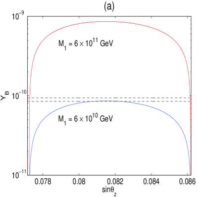
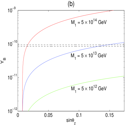
Figure 5.3: Numerical illustration of $Y_{\rm B}$ changing with $M_{1}$ and $\sin\theta_{z}$: (a) for the $m_{1}=0$ case; (b) for the $m_{3}=0$ case. The region between two dashed lines in (a) or (b) corresponds to the range of $Y_{\rm B}$ allowed by current observational data.

1. In the $m_{1}=0$ case, current data of $Y_{\rm B}$ require $M_{1}\geq 5.9\times 10^{10}~{}{\rm GeV}$ for the allowed ranges of $s_{z}$. Once $s_{z}$ is precisely measured, it is possible to fix the value of $M_{1}$ and then exclude some possibilities (e.g., the one with $M_{1}=10^{11}~{}{\rm GeV}$ will be ruled out, if $s_{z}\approx 0.082$ holds).

2. In the $m_{3}=0$ case, the condition $M_{1}\geq 3.8\times 10^{13}~{}{\rm GeV}$ is imposed by current data of $Y_{\rm B}$. Although $\theta_{z}$ is less restricted in this scenario, it remains possible to pin down the value of $M_{1}$ once $\theta_{z}$ is determined (e.g., $M_{1}\approx 5\times 10^{13}~{}{\rm GeV}$ is expected, if $s_{z}\approx 0.14$ holds).

A similar analysis of $Y_{\rm B}$ can be done in the supersymmetric version of the MSM.[36]

Note that we have simply used the low-energy values of light neutrino masses and flavor mixing angles in the above calculation of $\varepsilon_{1}$ and $Y_{\rm B}$. Now let us take into account the RGE running effects on these parameters from $\mu=M_{Z}$ up to $\mu=M_{1}$. With the help of Eq. (4.24), we can obtain an approximate relationship between $\varepsilon_{1}(M_{1})$ and $\varepsilon_{1}(M_{Z})$:[47]

$$\varepsilon_{1}(M_{1})\approx I^{-1}_{\alpha}\varepsilon_{1}(M_{Z})\;.$$ (5.39)

Looking at the running behavior of $I_{\alpha}$ shown in Fig. 4.2, we conclude that $\varepsilon_{1}$ is radiatively corrected by a factor smaller than two. Therefore, $\varepsilon_{1}(M_{1})\approx\varepsilon_{1}(M_{Z})$ is actually an acceptable approximation in the MSM.

In the flavor basis where both $M_{l}$ and $M_{\rm R}$ are diagonal, Eq. (5.2) shows that $\varepsilon_{1}$ only depends on the nontrivial phases of $M_{\rm D}$. This observation implies that there might not exist a direct connection between CP violation in heavy Majorana neutrino decays and that in light Majorana neutrino oscillations. The former is characterized by $\varepsilon_{i}$, while the latter is measured by the phase parameter $\delta$ of $V$ or more exactly by the Jarlskog invariant $J_{\rm CP}$. That is to say, $\varepsilon_{i}$ and $J_{\rm CP}$ (or $\delta$) seem not to be necessarily correlated with each other.[61] But their correlation is certainly possible in the MSM under discussion, in which $M_{\nu}$ is linked to $M_{\rm D}$ and $M_{\rm R}$. Taking account of the flavor effects in leptogenesis,[53] however, several authors have pointed out that CP violation at low energies is necessarily related to that at high energies in the canonical seesaw models.[62]

The correlation between leptogenesis and CP violation in neutrino oscillations has been discussed in the MSM.[25, 28, 36, 47] Here we illustrate how the cosmological baryon number asymmetry is correlated with the Jarlskog invariant of CP violation in the FGY ansatz. We plot the numerical result of $Y_{\rm B}$ versus $J_{\rm CP}$ in Fig. 5.4,[36] where $M_{1}=8\times 10^{10}~{}{\rm GeV}$ for the $m_{1}=0$ case and $M_{1}=6\times 10^{13}~{}{\rm GeV}$ for the $m_{3}=0$ case have typically been taken. One can see that the observationally-allowed range of $Y_{\rm B}$ corresponds to $J_{\rm CP}\sim 1\%$ in the $m_{1}=0$ case and $J_{\rm CP}\sim 2\%$ in the $m_{3}=0$ case. The correlation between $Y_{\rm B}$ and $J_{\rm CP}$ is so strong that it might be used to test the FGY ansatz after $J_{\rm CP}$ is measured in the future long-baseline neutrino oscillation experiments.

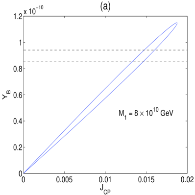
Figure 5.4: Numerical illustration of the correlation between $Y_{\rm B}$ and $J_{\rm CP}$: (a) in the $m_{1}=0$ case with $M_{1}=8\times 10^{10}~{}{\rm GeV}$; and (b) in the $m_{3}=0$ case with $M_{1}=6\times 10^{13}~{}{\rm GeV}$.

5.5 Lepton-Flavor-Violating Decays

The existence of neutrino oscillations implies the violation of lepton flavors. Hence the lepton-flavor-violating (LFV) decays in the charged-lepton sector, such as $\mu\to e+\gamma$, should also take place. They are unobservable in the SM, because their decay amplitudes are expected to be highly suppressed by the ratios of neutrino masses ($m_{i}\lesssim 1$ eV) to the $W$-boson mass ($M_{W}\approx 80$ GeV). In the supersymmetric extension of the SM, however, the branching ratios of such rare processes can be enormously enlarged. Current experimental bounds on the LFV decays $\mu\to e+\gamma$, $\tau\to e+\gamma$ and $\tau\to\mu+\gamma$ are[63]

$${\rm BR}(\mu\rightarrow e\gamma)\; < \;1.2\times 10^{-11}\;,$$

$${\rm BR}(\tau\rightarrow e\gamma)\; < \;1.1\times 10^{-7}\;,$$

$${\rm BR}(\tau\rightarrow\mu\gamma)\; < \;6.8\times 10^{-8}\;.$$ (5.40)

The sensitivities of a few planned experiments[64] may reach ${\rm BR}(\mu\rightarrow e\gamma)\sim 1.3\times 10^{-13}$, ${\rm BR}(\tau\rightarrow e\gamma)\sim{\cal O}(10^{-8})$ and ${\rm BR}(\tau\rightarrow\mu\gamma)\sim{\cal O}(10^{-8})$.

For simplicity, here we restrict ourselves to a very conservative case in which supersymmetry is broken in a hidden sector and the breaking is transmitted to the observable sector by a flavor blind mechanism, such as gravity.[23] Then all the soft breaking terms are diagonal at high energy scales, and the only source of lepton flavor violation in the charged-lepton sector is the radiative correction to the soft terms through the neutrino Yukawa couplings. In other words, the low-energy LFV processes $l_{j}\to l_{i}+\gamma$ are induced by the RGE effects of the slepton mixing. The branching ratios of $l_{j}\to l_{i}+\gamma$ are given by [24, 31]

$${\rm BR}(l_{j}\rightarrow l_{i}\gamma)\approx\frac{\alpha^{3}}{G^{2}_{\rm F}m^{8}_{\rm S}}\left[\frac{3m^{2}_{0}+A^{2}_{0}}{8\pi^{2}v^{2}\sin^{2}\beta}\right]^{2}|C_{ij}|^{2}\tan^{2}\beta\;,$$ (5.41)

where $m_{0}$ and $A_{0}$ denote the universal scalar soft mass and the trilinear term at $\Lambda_{\rm GUT}$, respectively. In addition,[65]

$$m^{8}_{\rm S}\;\approx\;0.5m^{2}_{0}M^{2}_{1/2}(m^{2}_{0}+0.6M^{2}_{1/2})^{2}\;$$ (5.42)

with $M_{1/2}$ being the gaugino mass; and

$$C_{ij}\;=\;\sum_{k}(M_{\rm D})_{ik}(M^{*}_{\rm D})_{jk}{\rm ln}\frac{\Lambda_{\rm GUT}}{M_{k}}\;$$ (5.43)

with $\Lambda_{\rm GUT}=2.0\times 10^{16}$ GeV to be fixed in our calculations. The LFV decays have been discussed in the supersymmetric version of the MSM.[23, 35, 40, 66] To illustrate, we are going to compute the LFV processes by taking account of the FGY ansatz, which only has three unknown parameters $\theta_{z}$, $M_{1}$ and $M_{2}$.

To calculate the branching ratio of $\mu\rightarrow e+\gamma$, we need to know the following parameters in the framework of the minimal supergravity (mSUGRA) model: $M_{1/2}$, $m_{0}$, $A_{0}$, $\tan\beta$ and ${\rm sign}(\mu)$. These parameters can be constrained from cosmology (by demanding that the proper supersymmetric particles should give rise to an acceptable dark matter density) and low-energy measurements (such as the process $b\rightarrow s+\gamma$ and the anomalous magnetic moment of muon $g_{\mu}-2$). Here we adopt the Snowmass Points and Slopes [67] (SPS) listed in Table. 5.1. These points and slopes are a set of benchmark points and parameter lines in the mSUGRA parameter space corresponding to different scenarios in the search for supersymmetry at present and future experiments. Points 1a and 1b are “typical” mSUGRA points (with intermediate and large $\tan\beta$, respectively), and they lie in the “bulk” of the cosmological region where the neutralino is sufficiently light and no specific suppression mechanism is needed. Point 2 lies in the “focus point” region, where a too large relic abundance is avoided by an enhanced annihilation cross section of the lightest supersymmetric particle (LSP) due to a sizable higgsino component. Point 3 is directed towards the co-annihilation region where the LSP is quasi-degenerate with the next-to-LSP (NLSP). A rapid co-annihilation between the LSP and the NLSP can give a sufficiently low relic abundance. Points 4 and 5 are extreme $\tan\beta$ cases with very large and small values, respectively.

Point	$M_{1/2}$	$m_{0}$	$A_{0}$	$\tan\beta$	Slope
1 a	250	100	-100	10	$m_{0}=-A_{0}=0.4M_{1/2}$, $M_{1/2}$ varies
1 b	400	200	0	30
2	300	1450	0	10	$m_{0}=2M_{1/2}+850$ GeV, $M_{1/2}$ varies
3	400	90	0	10	$m_{0}=0.25M_{1/2}-10$ GeV, $M_{1/2}$ varies
4	300	400	0	50
5	300	150	-1000	5

Table 5.1: Some parameters for the SPS in the mSUGRA. The masses are given in unit of GeV. $\mu$ appearing in the Higgs mass term has been taken as $\mu>0$ for all SPS.

With the help of Eqs. (4.5) and (5.41), $|C_{ij}|^{2}$ can explicitly be written as

$$|C_{12}|^{2} = |a_{1}|^{2}\;|a_{2}|^{2}\;\left(\displaystyle{\rm ln}\frac{\Lambda_{\rm GUT}}{M_{1}}\right)^{2}\;,$$

$$|C_{13}|^{2} = 0\;,$$

$$|C_{23}|^{2} = |b_{2}|^{2}\;|b_{3}|^{2}\;\left(\displaystyle{\rm ln}\frac{\Lambda_{\rm GUT}}{M_{2}}\right)^{2}\;.$$ (5.44)

Because of $|C_{13}|^{2}=0$, we are left with ${\rm BR}(\tau\rightarrow e\gamma)=0$. If ${\rm BR}(\tau\rightarrow e\gamma)\neq 0$ is established from the future experiments, it will be possible to exclude the FGY ansatz. Using Eq. (5.35), we reexpress Eq. (5.42) as

$$|C_{12}|^{2} = M_{1}^{2}\;|(M_{\nu})_{12}|^{2}\;\left(\displaystyle{\rm ln}\frac{\Lambda_{\rm GUT}}{M_{1}}\right)^{2}\;,$$

$$|C_{23}|^{2} = M_{2}^{2}\;|(M_{\nu})_{23}|^{2}\;\left(\displaystyle{\rm ln}\frac{\Lambda_{\rm GUT}}{M_{2}}\right)^{2}\;.$$ (5.45)

As shown in Sec. 5.4, $M_{1}$ may in principle be constrained by leptogenesis for given values of $\sin\theta_{z}$. For simplicity, we choose $Y_{\rm B}=9.0\times 10^{-11}$ as an input parameter, but $M_{2}$ is entirely unrestricted from the successful leptogenesis with $M_{2}\gg M_{1}$.

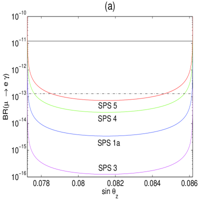
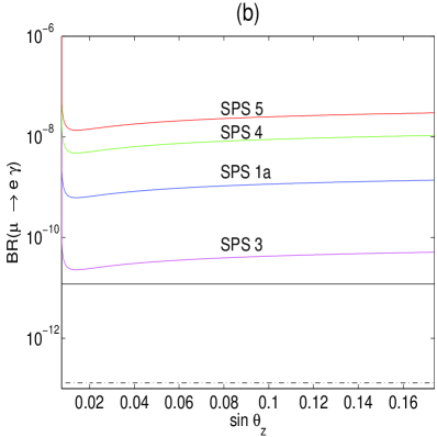
Figure 5.5: Numerical illustration of the dependence of ${\rm BR}(\mu\rightarrow e\gamma)$ on $\sin\theta_{z}$: (a) in the $m_{1}=0$ case; and (b) in the $m_{3}=0$ case. The black solid line and black dash-dot line denote the present experimental upper bound on and the future experimental sensitivity to ${\rm BR}(\mu\rightarrow e\gamma)$, respectively.

We numerically calculate BR($\mu\rightarrow e\gamma$) for different values of $\sin\theta_{z}$ by using the SPS points. The results are shown in Fig. 5.5. Since the SPS points 1a and 1b (or Points 2 and 3) almost have the same consequence in our scenario, we only focus on Point 1a (or Point 3). When $\sin\theta_{z}\rightarrow 0.077$ or $\sin\theta_{z}\rightarrow 0.086$, the future experiment is likely to probe the branching ratio of $\mu\rightarrow e+\gamma$ in the $m_{1}=0$ case. The reason is that $\sin\theta_{z}\rightarrow 0.077$ (or $\sin\theta_{z}\rightarrow 0.086$) implies $\phi\rightarrow-\pi/2$ (or $\phi\rightarrow 0$). Furthermore, the successful leptogenesis requires a very large $M_{1}$ due to $\varepsilon_{1}\propto\sin 2\phi$. It is clear that the SPS points are all unable to satisfy ${\rm BR}(\mu\rightarrow e\gamma)\leq 1.2\times 10^{-11}$ in the $m_{3}=0$ case. Therefore, we can exclude the $m_{3}=0$ case when the SPS points are taken as the mSUGRA parameters. When $\sin\theta_{z}\simeq 0.014$, ${\rm BR}(\mu\rightarrow e\gamma)$ arrives at its minimal value in the $m_{3}=0$ case. For the SPS slopes, larger $M_{1/2}$ yields smaller ${\rm BR}(\mu\rightarrow e\gamma)$. We plot the numerical dependence of BR($\mu\rightarrow e\gamma$) on $M_{1/2}$ in Fig. 5.6, where we have adopted the SPS slope 3 and taken $300~{}{\rm GeV}\leq M_{1/2}\leq 1000~{}{\rm GeV}$. We find that $M_{1/2}\geq 474~{}{\rm GeV}$ (or $M_{1/2}\geq 556~{}{\rm GeV}$) can result in ${\rm BR}(\mu\rightarrow e\gamma)\leq 1.2\times 10^{-11}$ for $\sin\theta_{z}=0.014$ (or $\sin\theta_{z}=0.1$). For all values of $M_{1/2}$ between 300 GeV and 1000 GeV, ${\rm BR}(\mu\rightarrow e\gamma)$ is larger than the sensitivity of some planned experiments, which ought to examine the $m_{3}=0$ case when the SPS slope 3 is adopted. The same conclusion can be drawn for the SPS slopes 1a and 2. In view of the present experimental results on muon $g_{\mu}-2$, one may get $M_{1/2}\lesssim 430$ GeV for $\tan\beta=10$ and $A_{0}=0$,[68] implying that the $m_{3}=0$ case should be disfavored.

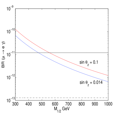
Figure 5.6: Numerical illustration of the dependence of ${\rm BR}(\mu\rightarrow e\gamma)$ on $M_{1/2}$ for SPS slope 3 in the $m_{3}=0$ case. The black solid line and black dash-dot line denote the present experimental upper bound on and the future experimental sensitivity to ${\rm BR}(\mu\rightarrow e\gamma)$, respectively.

With the help of Eqs. (5.39) and (5.43), one can obtain

$$\frac{{\rm BR}(\tau\rightarrow\mu\gamma)}{{\rm BR}(\mu\rightarrow e\gamma)}\;=\;\frac{M_{2}^{2}\;|(M_{\nu})_{23}|^{2}\;\left[{\rm ln}({\Lambda_{\rm GUT}}/{M_{2}})\right]^{2}}{M_{1}^{2}\;|(M_{\nu})_{12}|^{2}\;\left[{\rm ln}({\Lambda_{\rm GUT}}/{M_{1}})\right]^{2}}\;\;.$$ (5.46)

Since the successful leptogenesis can be used to fix $M_{1}$, a measurement of the above ratio will allow us to determine or constrain $M_{2}$. It is worth remarking that this ratio is independent of the mSUGRA parameters. To illustrate, we show the numerical result of ${\rm BR}(\tau\rightarrow\mu\gamma)/{\rm BR}(\mu\rightarrow e\gamma)$ in Fig. 5.7 for both $m_{1}=0$ and $m_{3}=0$ cases. Below $\Lambda_{\rm GUT}$, the term $M_{2}^{2}[{\rm ln}(\Lambda_{\rm GUT}/{M_{2}})]^{2}$ and the ratio in Eq. (5.44) reach their maximum values at $M_{2}=\Lambda_{\rm GUT}/e=7.4\times 10^{15}$ GeV. Obviously, the ratio ${\rm BR}(\tau\rightarrow\mu\gamma)/{\rm BR}(\mu\rightarrow e\gamma)$ is below $2\times 10^{9}$ in the $m_{1}=0$ case and below $8\times 10^{3}$ in the $m_{3}=0$ case. This conclusion is independent of the mSUGRA parameters.[70]

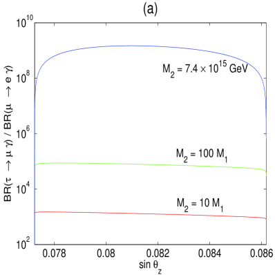
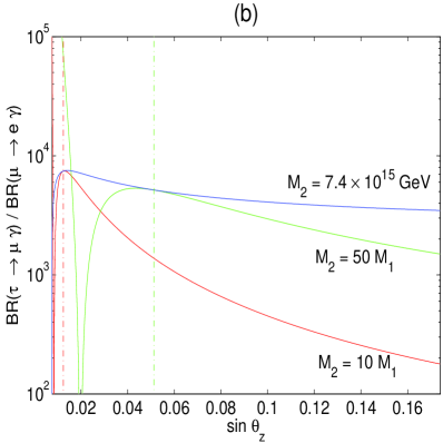
Figure 5.7: Numerical illustration of the dependence of ${\rm BR}(\tau\rightarrow\mu\gamma)/{\rm BR}(\mu\rightarrow e\gamma)$ on $\sin\theta_{z}$: (a) in the $m_{1}=0$ case; and (b) in the $m_{3}=0$ case.

6 Concluding Remarks

We have presented a review of recent progress in the study of the MSM, which only contains two heavy right-handed Majorana neutrinos. The attractiveness of this economical seesaw model is three-fold:

• Its consequences on neutrino phenomenology are almost as rich as those obtained from the conventional seesaw models with three heavy right-handed Majorana neutrinos. In particular, the MSM can simultaneously account for two kinds of new physics beyond the SM: the cosmological matter-antimatter asymmetry and neutrino oscillations.

• Its predictability and testability are actually guaranteed by its simplicity. For example, the neutrino mass spectrum in the MSM is essentially fixed, although current experimental data remain unable to tell whether $m_{1}=0$ or $m_{3}=0$ is really true or close to the truth.

• Its supersymmetric version allows us to explore a wealth of new phenomena at both low- and high-energy scales. On the one hand, certain flavor symmetries can be embedded in the supersymmetric MSM; on the other hand, the rare LFV processes can naturally take place in such interesting scenarios.

Therefore, we are well motivated to outline the salient features of the MSM and summarize its various phenomenological implications in this article.

In view of current neutrino oscillation data, we have demonstrated that the MSM can predict the neutrino mass spectrum and constrain the effective masses of the tritium beta decay and the neutrinoless double-beta decay. Five distinct parameterization schemes have been introduced to describe the neutrino Yukawa-coupling matrix of the MSM. We have investigated neutrino mixing and baryogenesis via leptogenesis in some detail by taking account of possible texture zeros of the Dirac neutrino mass matrix. An upper bound on the CP-violating asymmetry in the decay of the lighter right-handed Majorana neutrino has been derived. The RGE running effects on neutrino masses, flavor mixing angles and CP-violating phases have been analyzed, and the correlation between the CP-violating phenomena at low and high energies has been highlighted. It has been shown that the observed matter-antimatter asymmetry of the Universe can naturally be interpreted through the resonant leptogenesis mechanism at the TeV scale. The LFV decays, such as $\mu\to e+\gamma$, have also been discussed in the supersymmetric extension of the MSM.

Of course, there remain many open questions in neutrino physics. But we are paving the way to eventually answer them. No matter whether the MSM can survive the experimental and observational tests in the near future, we expect that it may provide us with some valuable hints in looking for the complete theory of massive neutrinos.

References

- [1] SNO Collaboration, Q. R. Ahmad et al., Phys. Rev. Lett. 89 (2002) 011301.
- [2] For a review, see: C. K. Jung et al., Ann. Rev. Nucl. Part. Sci. 51 (2001) 451.
- [3] KamLAND Collaboration, K. Eguchi et al., Phys. Rev. Lett. 90 (2003) 021802; CHOOZ Collaboration, M. Apollonio et al., Phys. Lett. B420 (1998) 397; Palo Verde Collaboration, F. Boehm et al., Phys. Rev. Lett. 84 (2000) 3764.
- [4] K2K Collaboration, M. H. Ahn et al., Phys. Rev. Lett. 90 (2003) 041801.
- [5] P. Minkowski, Phys. Lett. B67 (1977) 421; T. Yanagida, in Proceedings of the Workshop on Unified Theory and the Baryon Number of the Universe, edited by O. Sawada and A. Sugamoto (KEK, Tsukuba, 1979); M. Gell-Mann, P. Ramond and R. Slansky, in Supergravity, edited by P. van Nieuwenhuizen and D. Freedman (North Holland, Amsterdam, 1979); S. L. Glashow, in Quarks and Leptons, edited by M. Lvy et al. (Plenum, New York, 1980); R. N. Mohapatra and G. Senjanovic, Phys. Rev. Lett. 44 (1980) 912.
- [6] See, e.g., T. P. Cheng and L. F. Li, Phys. Rev. D22 (1980) 2860; J. Schechter and J. W. F. Valle, Phys. Rev. D22 (1980) 2227.
- [7] A. D. Sakharov, JETP Lett. 5 (1967) 24.
- [8] M. Fukugita and T. Yanagida, Phys. Lett. B174 (1986) 45.
- [9] G. ’t Hooft, Phys. Rev. Lett. 37 (1976) 8; F. R. Klinkhamer and N. S. Manton, Phys. Rev. D30 (1984) 2212; V. A. Kuzmin, V. A. Rubakov and M. E. Shaposhnikov, Phys. Lett. B155 (1985) 36.
- [10] P. H. Frampton, S. L. Glashow and T. Yanagida, Phys. Lett. B548 (2002) 119. Earlier works on the seesaw mechanism with two heavy right-handed Majorana neutrinos can be found: A. Kleppe, in Proceedings of the Workshop on What Comes Beyond the Standard Model, Bled, Slovenia, 29 June - 9 July 1998; L. Lavoura and W. Grimus, JHEP 0009 (2000) 007.
- [11] A. Pilaftsis, Phys. Rev. D56 (1997) 5431; Int. J. Mod. Phys. A14 (1999) 1811; A. Pilaftsis and T. E. J. Underwood, Nucl. Phys. B692 (2004) 303.
- [12] Z. Z. Xing and S. Zhou, High Energy Phys. Nucl. Phys. 30 (2006) 828.
- [13] Z. Maki, M. Nakagawa and S. Sakata, Prog. Theor. Phys. 28 (1962) 870.
- [14] Particle Data Group, W. M. Yao et al., J. Phys. G33 (2006) 1.
- [15] A. Strumia and F. Vissani, Nucl. Phys. B26 (2005) 294; hep-ph/0606054.
- [16] S. M. Bilenky, C. Giunti, J. A. Grifols and E. Mass, Phys. Rept. 379 (2003) 69; and references therein.
- [17] See, e.g., Z. Z. Xing, Int. J. Mod. Phys. A19 (2004) 1; and references therein.
- [18] L. Wolfenstein, in Proc. of Neutrino 84, p. 730; F. Vissani, JHEP 9906 (1999) 022; S. M. Bilenky, S. Pascoli and S. T. Petcov, Phys. Rev. D64 (2001) 053010; W. Rodejohann, Nucl. Phys. B597 (2001) 110; F. Feruglio, A. Strumia and F. Vissani, Nucl. Phys. B637 (2002) 345; S. Pascoli, S. T. Petcov and L. Wolfenstein, Phys. Lett. B524 (2002) 319.
- [19] Z. Z. Xing, Phys. Rev. D68 (2003) 053002.
- [20] W. L. Guo and Z. Z. Xing, High Energy Phys. Nucl. Phys. 30 (2006) 709.
- [21] Heidelberg-Moscow Collaboration, H. V. Klapdor-Kleingrothaus, hep-ph/0103074; C. E. Aalseth et al., Phys. Rev. D65 (2002) 092007; and references cited therein.
- [22] KATRIN Collaboration, A. Osipowicz et al., hep-ex/0109033.
- [23] A. Ibarra and G. G. Ross, Phys. Lett. B591 (2004) 285.
- [24] J. A. Casas and A. Ibarra, Nucl. Phys. B618 (2001) 171.
- [25] S. Blanchet and P. Di Bari, JCAP 0606 (2006) 023.
- [26] R. Gonzalez Felipe, F. R. Joaquim and B. M. Nobre, Phys. Rev. D70 (2004) 085009.
- [27] K. Turzynski, Phys. Lett. B589 (2004) 135.
- [28] T. Endoh, S. Kaneko, S. K. Kang, T. Morozumi and M. Tanimoto, Phys. Rev. Lett. 89 (2002) 231601.
- [29] V. Barger, D. A. Dicus, H. J. He and T. J. Li, Phys. Lett. B583 (2004) 173.
- [30] A. Ibarra, JHEP 0601 (2006) 064.
- [31] J. Hisano, T. Moroi, K. Tobe, M. Yamaguchi and T. Yanagida, Phys. Lett. B357 (1995) 579; J. Hisano, T. Moroi, K. Tobe and M. Yamaguchi, Phys. Rev. D53 (1996) 2442.
- [32] B. C. Regan, E. D. Commins, C. J. Schmidt and D. DeMille, Phys. Rev. Lett. 88 (2002) 071805.
- [33] T. Fujihara, S. Kaneko, S. K. Kang, D. Kimura, T. Morozumi and M. Tanimoto, Phys. Rev. D72 (2005) 016006.
- [34] K. Bhattacharya, N. Sahu, U. Sarkar and S. K. Singh, hep-ph/0607272.
- [35] M. Raidal and A. Strumia, Phys. Lett. B553 (2003) 72.
- [36] W. L. Guo and Z. Z. Xing, Phys. Lett. B583 (2004) 163.
- [37] Z. Z. Xing, Phys. Lett. B530 (2002) 159; P. H. Frampton, S. L. Glashow and D. Marfatia, Phys. Lett. B536 (2002) 79; Z. Z. Xing, Phys. Lett. B539 (2002) 85; A. Kageyama, S. Kaneko, N. Shimoyama and M. Tanimoto, Phys. Lett. B538 (2002) 96; W. L. Guo and Z. Z. Xing, Phys. Rev. D67 (2003) 053002; Z. Z. Xing and H. Zhang, Phys. Lett. B569 (2003) 30; Z. Z. Xing, Phys. Rev. D69 (2004) 013006; Z. Z. Xing and H. Zhang, J. Phys. G30 (2004) 129; S. Zhou and Z. Z. Xing, Eur. Phys. J. C38 (2005) 495; Z. Z. Xing and S. Zhou, Phys. Lett. B606 (2005) 145.
- [38] For recent reviews with extensive references, see: H. Fritzsch and Z. Z. Xing, Prog. Part. Nucl. Phys. 45 (2000) 1; V. Barger, D. Marfatia and K. Whisnant, Int. J. Mod. Phys. E12 (2003) 569; G. Altarelli and F. Feruglio, New J. Phys. 6 (2004) 106; R. N. Mohapatra and A. Yu. Smirnov, hep-ph/0603118.
- [39] S. Raby, Phys. Lett. B561 (2003) 119.
- [40] R. Kuchimanchi and R. N. Mohapatra, Phys. Rev. D66 (2002) 051301; Phys. Lett. B552 (2003) 198; B. Dutta and R. N. Mohapatra, Phys. Rev. D68 (2003) 056006.
- [41] S. Chang, S. K. Kang and K. Siyeon, Phys. Lett. B597 (2004) 78.
- [42] G. C. Branco, M. N. Rebelo and J. I. Silva-Marcos, Phys. Lett. B633 (2006) 345.
- [43] R. N. Mohapatra and S. Nasri, Phys. Rev. D71 (2005) 033001.
- [44] C. Jarlskog, Phys. Rev. Lett. 55 (1985) 1039; D.D. Wu, Phys. Rev. D33 (1986) 860.
- [45] Z. Z. Xing, Phys. Rev. D69 (2004) 013006.
- [46] See, e.g., J. A. Casas, J. R. Espinosa, A. Ibarra and I. Navarro, Nucl. Phys. B569 (2000) 82; B573 (2000) 652; P. H. Chankowski and S. Pokorski, Int. J. Mod. Phys. A17 (2002) 575; S. Antusch, J. Kersten, M. Lindner and M. Ratz, Nucl. Phys. B674 (2003) 401; S. Antusch, J. Kersten, M. Lindner, M. Ratz and M. A. Schmidt, JHEP 0503 (2005) 024; J. W. Mei, Phys. Rev. D71 (2005) 073012.
- [47] J. W. Mei and Z. Z. Xing, Phys. Rev. D69 (2004) 073003.
- [48] J. R. Ellis and S. Lola, Phys. Lett. B458 (1999) 310; Z. Z. Xing, Phys. Rev. D63 (2001) 057301.
- [49] D. N. Spergel et al., astro-ph/0603449.
- [50] For a recent review with extensive references, see: M. Dine and A. Kusenko, Rev. Mod. Phys. 76 (2004) 1.
- [51] J. Ellis, M. Raidal and T. Yanagida, Phys. Lett. B546 (2002) 228; and references therein.
- [52] M. A. Luty, Phys. Rev. D45 (1992) 455; M. Flanz, E. A. Paschos and U. Sarkar, Phys. Lett. B345 (1995) 248; L. Covi, E. Roulet and F. Vissani, Phys. Lett. B384 (1996) 169; M. Flanz, E. A. Paschos, U. Sarkar and J. Wess, Phys. Lett. B389 (1996) 693; M. Plmacher, Z. Phys. C74 (1997) 549; A. Pilaftsis, Phys. Rev. D56 (1997) 5431; Int. J. Mod. Phys. A14 (1999) 1811; W. Buchmller and M. Plmacher, Phys. Lett. B431 (1998) 354; M. Plmacher, Nucl. Phys. B530 (1998) 207; R. Barbieri, P. Creminelli, A. Strumia and N. Tetradis, Nucl. Phys. B575 (2000) 61; T. Hambye, Nucl. Phys. B633 (2002) 171; W. Buchmller, P. Di Bari and M. Plmacher, Nucl. Phys. B643 (2002) 367; G. F. Giudice, A. Notari, M. Raidal, A. Riotto and A. Strumia, Nucl. Phys. B685 (2004) 89.
- [53] A. Abada, S. Davidson, F. X. Josse-Michaux, M. Losada and A. Riotto, JCAP 0604 (2006) 004; hep-ph/0605281; E. Nardi, Y. Nir, E. Roulet and J. Racker, JHEP 0601 (2006) 164; S. Blanchet and P. Di Bari, hep-ph/0607330; S. Antusch, S. F. King and A. Riotto, hep-ph/0609038; S. Blanchet, P. Di Bari and G. G. Raffelt, hep-ph/0611337; A. De Simone and A. Riotto, hep-ph/0611357; S. Pascoli, S. T. Petcov and A. Riotto, hep-ph/0611338.
- [54] E. W. Kolb and M. S. Turner, The Early Universe, Addison-Wesley (1990); H. B. Nielsen and Y. Takanishi, Phys. Lett. B507 (2001) 241; E. Kh. Akhmedov, M. Frigerio and A. Yu. Smirnov, JHEP 0309 (2003) 021; Z. Z. Xing, Phys. Rev. D70 (2004) 071302.
- [55] J. A. Harvey and M. S. Turner, Phys. Rev. D42 (1990) 3344.
- [56] S. Davidson and A. Ibarra, Phys. Lett. B535 (2002) 25; W. Buchmller, P. Di Bari and M. Plmacher, Nucl. Phys. B643 (2002) 367.
- [57] J. Ellis, D. V. Nanopoulos and S. Sarkar, Nucl. Phys. B259 (1985) 175.
- [58] Z. Z. Xing and S. Zhou, hep-ph/0607302.
- [59] P. F. Harrison, D. H. Perkins and W.G. Scott, Phys. Lett. B530 (2002) 167; Z. Z. Xing, Phys. Lett. B533 (2002) 85; P. F. Harrison and W. G. Scott, Phys. Lett. B535 (2002) 163; X. G. He and A. Zee, Phys. Lett. B560 (2003) 87.
- [60] W. Buchmller, P. Di Bari and M. Plmacher, New J. Phys. 6 (2004) 105; G. F. Giudice, A. Notari, M. Raidal, A. Riotto and A. Strumia, in Ref. 51.
- [61] W. Buchmller and M. Plmacher, Phys. Lett. B389 (1996) 73.
- [62] S. Pascoli, S. T. Petcov and A. Riotto, hep-ph/0609125; G. C. Branco, R. Gonzalez-Felipe and F. R. Joaquim, hep-ph/0609297.
- [63] MEGA Collaboration, M. L. Brooks et al., Phys. Rev. Lett. 83 (1999) 1521; BABAR Collaboration, B. Aubert et al., Phys. Rev. Lett. 96 (2006) 041801; BABAR Collaboration B. Aubert et al., Phys. Rev. Lett. 95 (2005) 041802;
- [64] SuperKEKB Physics Working Group, A. G. Akeroyd et al., hep-ex/0406071; S. Ritt, http://meg.web.psi.ch/docs/talks/sritt/mar06novosibirsk/ritt.ppt.
- [65] S. T. Petcov, S. Profumo, Y. Takanishi and C. E. Yaguna, Nucl. Phys. B676 (2004) 453.
- [66] J. J. Cao, Z. H. Xiong and J. M. Yang, Eur.Phys.J. C32 (2004) 245.
- [67] B. C. Allanach et al., Eur. Phys. J. C25 (2002) 113.
- [68] J. Ellis, K. A. Olive, Y. Santoso and V. C. Spanos, Phys. Lett. B565 (2003) 176; M. Battaglia, A. De Roeck, J. Ellis, F. Gianotti, K. A. Olive and L. Pape, Eur. Phys. J. C33 (2004) 273.
- [69] The LEP Higgs Working Group, hep-ex/0107030.
- [70] W. L. Guo, hep-ph/0610174.