High energy hadron production Monte Carlos

Abstract

We discuss here Quantum molecular dynamics models (QMD) and Dual Parton Models ( DPM and QGSM). We compare RHIC data to DPM–models and we present a (Cosmic ray oriented) model comparison.

1 Quantum molecular dynamics models (QMD)

The emphasis of this contribution is to high energies, therefore, QMD non–relativistic models ($E<2AGeV$) are not treated here.

The first relativistic QMD model was RQMD Sorge89a. This model is no longer supported since the year 2000 ,RQMD is used in FLUKA for A–A collisions below 5AGeV.

A second relativistic model is UrQMD Bass98, it is used in CORSIKA Cosmic Ray cascade code below 80AGeV.

Let me mention some efforts within the FLUKA collaboration which will not be treated here: F.Cerutti et al. add (approximate) energy conservation , evaporation, and residual nuclei to RQMD Cerutti04. M.V.Garzelli et al. construct a low enery QMD for A–A collisions in FLUKA Garzelli06. There are efforts in Milano and Houston to construct a fully relativistic model for A–A collisions to be inserted into FLUKA.

A relativistic QMD model is a Lorentz invariant cascade (molecular dynamics) with nucleons of both nuclei and all produced hadrons as participants. Properties of such models are: (i)A formation zone cascade of all produced hadrons. (ii) Elementary interactions used in the models include: (1) h + h $\longrightarrow$ resonance; resonance + resonance and resonance decay (similar to HADRIN in FLUKA), (2) high enery: h + h $\longrightarrow$ hadronic chain; 2 hadronic chains and Lund like chain fragmentation, (3) chain fusion (called formation of color ropes) in RQMD, (4) empirical parametrization of all cross sections, (5) pQCD description of hard collisions (UrQMD).

1.1 The kinematics of the UrQMD model

The model is fully described in Bass98. It is based on the covariant propagation of all hadrons on classical trajectories in combination with stochastic binary scatterings, color string formation and resonance decay. It includes the Monte Carlo solution of a set of coupled partial integro-differential equations. Each nucleon is represented by a coherent state ($\hbar,c=1$)

$$\phi_{i}(\vec{x};\vec{q}_{i},\vec{p}_{i},t)=\left({\frac{2}{L\pi}}\right)^{3/4}\,\exp\left\{-\frac{2}{L}(\vec{x}-\vec{q}_{i}(t))^{2}+{\rm i}\vec{p}_{i}(t)\vec{x}\right\}$$ (1)

which is characterized by 6 time-dependent parameters, $\vec{q}_{i}$ and $\vec{p}_{i}$. $L$, (the extension of the wave packet in coordinate space) is fixed. The total $n$-body wave function is a product of coherent states (1) $\Phi=\prod_{i}\phi_{i}(\vec{x},\vec{q_{i}},\vec{p_{i}},t)$. The Hamiltonian $H$ of the system contains a kinetic term and mutual interactions $V_{ij}$ ($H=\sum_{i}T_{i}+{\ \frac{1}{2}}\sum_{ij}V_{ij}$). This yields an Euler-Lagrange equation for each parameter.

$$\dot{\vec{p}}_{i}=-\frac{\partial\langle H\rangle}{\partial\vec{q}_{i}}\quad{\rm and}\quad\dot{\vec{q}}_{i}=\frac{\partial\langle H\rangle}{\partial\vec{p}_{i}}\,.$$ (2)

These are the time evolution equations which are solved numerically. The UrQMD Hamiltonian contains: $E_{kin},E^{Sk2}_{jk},E^{Sk3}_{jkl},E^{Yukawa}_{jk},E^{Coulomb}_{jk},E^{Pauli}_{jk}$.

Please note: As one sees from the Hamiltonian UrQMD is not really a Lorentz invariant molecular dynamics. Therefore, the results of the model might depend strongly on the reference frame in which the calculation is done. To minimize this frame dependence the authors Bass98 use a frame–independent definition of the cross sections (via using the impact parameters in the two–particle rest frames). They give as example for this minimization in S–S collisions: The multiplicities and collision numbers vary only by less than 3% between the lab and CM frames.

Let us mention, that RQMD has a manifestly Lorentz invariant eq. of motion. Using 4–vectors for positions and momenta, each particle carries its own time. The 2N additional degrees of freedom are fixed by 2N constraints: The N mass shell constraints: $H_{i}=p_{i}^{2}-m_{i}^{2}-V_{i}=0$, ($V_{i}$: quasi potential) and (N-1) time fixations. The 2Nth constraint: A relation of times of particles to the evolution parameter $\tau$.

Projectile or target nucleus are modeled according to a Fermi-gas ansatz. The centroids of the Gaussians are randomly distributed within a sphere with the radius $R(A)$,

$$R(A)\,=\,r_{0}\left(\frac{1}{2}\left[A+\left(A^{\frac{1}{3}}-1\right)^{3}\right]\right)^{\frac{1}{3}}\,~{}~{}~{}~{}~{}r_{0}\,=\,\left(\frac{3}{4\pi\rho_{0}}\right)^{\frac{1}{3}}\,.$$ (3)

$\rho_{0}$ is the nuclear matter ground state density. If the phase-space density at the location of each nucleon is too high (i.e. the area of the nucleus is already occupied), then the location of that nucleon is rejected and a new location is randomly chosen. The initial momenta of the nucleons are randomly chosen between 0 and the local Thomas-Fermi-momentum: $p_{F}^{max}\,=\,\hbar c\left(3\pi^{2}\rho\right)^{\frac{1}{3}}$, with $\rho$ being the corresponding local proton- or neutron-density. One disadvantage of this type of initialization: the initialized nuclei are not in their ground-state with respect to the Hamiltonian used for the propagation. The parameters of the Hamiltonian are tuned to the equation of state of infinite nuclear matter and to properties of finite nuclei (such as their binding energy and their root mean square radius). One can use a so-called Pauli-potential in the Hamiltonian: This has the advantage that the initialized nuclei remain stable whereas in UrQMD with the conventional initialization and propagation without the Pauli-potential the nuclei start evaporating single nucleons after approximately 20 - 30 fm/c. One drawback of this potential: the kinetic momenta of the nucleons are not anymore equivalent to their canonic momenta, i.e. the nucleons carry the correct Fermi-momentum, but their velocity is zero. The impact parameter of a collision is sampled according to the quadratic measure ($dW\sim~{}bdb$). At a given impact parameter the centers of projectile and target are placed along the collision axis in such a manner that a distance between surfaces of the projectile and the target is equal to 3 $fm$. The momenta of the nucleons are transformed into the system where the projectile and target have equal velocities directed in opposite directions of the axis. After that the time propagation starts. During the calculation each particle is checked at the beginning of each time step whether it will collide within that time step.

The relativistic QMD models are compared to a large sample of data in the publications of the authors. Up to energies of about $\sqrt{s}$ = 200 GeV usually a good agreement is found. The experimental collaborations at RHIC compare their data quite often to RQMD results, One example: The PHOBOS Collaboration in their white paper PHOBOS02a find a good agreement to $dN_{ch}/dy$ from RQMD for Au–Au collisions to their data, the reason for this is the chain fusion build from the beginning into RQMD.

The main problems of the relativistic QMD models, which make them difficult to apply for shower simulations are (i) problems with the energy conservation, (ii) the missing evaporation and residual nuclei and (iii) the partly excessive computer running times.

2 DPM and QGSM models

The Dual Parton Model DPM and the Quark Gluon String Model QGSM are two models, which are largely equivalent in their construction, only with some characteristic differences. The DPM is due to Capella, Tran Than Van and collaborators DPMREV92. The most detailled Monte Carlo versions of the DPM are PHOJET Engel95a; Engel95d for h–h and $\gamma$–h collisions and DPMJET for h–A, A–A and $\gamma$–A collisions Roesler20002.

The QGSM is due to Kaidalov, Ter-Martyrosian and collaborators Kaidalov82b. The Monte Carlo version QGSJET for h–h, h–A and A–A collisions is due to Kalmykov, Ostapchenko and collaborators QGSJET.

2.1 The construction of the PHOJET multichain model

We restrict us in this contribution to describe the PHOJET model, which is used directly for h–h collisions and for all elementary Glauber collisions in h–A and A–A collisions in DPMJET . There are no essential differences in the formulations of the Glauber model between different Monte Carlo models.

The (soft) Born cross section of the supercritical pomeron has the form $\sigma_{s}=g^{2}s^{\alpha(0)-1}$. The supercritical pomeron has $\alpha(0)>1.$, therefore it clearly violates unitarity. According to the Froissart bound the cross section asymptotically should not rise faster than ${(\log s)}^{2}$.

If we start to construct the full model, which is unitarized, we should introduce some more input Born cross sections. Very important is the hard cross section, which we calculate according to the QCD improved parton model:

$$\sigma^{\mbox{hard}}(s,p_{\perp}^{\mbox{cutoff}})=\int dx_{1}dx_{2}d\hat{t}\sum_{i,j,k,l}\frac{1}{1+\delta_{k,l}}$$

$$f_{a,i}(x_{1},Q^{2})f_{b,j}(x_{2},Q^{2})\frac{d\sigma_{i,j\rightarrow k,l}^{\mbox{QCD}}(\hat{s},\hat{t})}{d\hat{t}}\Theta(p_{\perp}-p_{\perp}^{\mbox{cutoff}}),$$ (4)

where $f_{a,i}(x_{1},Q^{2})$ is the distribution of the parton $i$ in $a$.

One of the most important difference between PHOJET/DPMJET and QGSJET is in the $p_{\perp}$ cutoff $p_{\perp}^{\mbox{cutoff}}$: PHOJET/DPMJET use $p_{\perp}^{\mbox{cutoff}}$ rising with energy. QGSJET uses $p_{\perp}^{\mbox{cutoff}}$ constant, independent of the energy.

We introduce furthermore the cross sections for high–mass single and double diffraction $\sigma_{D}$ and for high–mass central diffraction $\sigma_{C}$ according to the standard expressions. The amplitudes corresponding to the one-pomeron exchange are unitarized applying an eikonal formalism. In impact parameter representation, the eikonalized scattering amplitude has the structure

$$a(s,B)=\frac{i}{2}\left(\frac{e^{2}}{f^{2}_{q\bar{q}}}\right)^{2}\;\left(1-e^{-\chi(s,B)}\right)$$ (5)

with the eikonal function

$$\chi(s,B)=\chi_{S}(s,B)+\chi_{H}(s,B)+\chi_{D}(s,B)+\chi_{C}(s,B).$$ (6)

Here, $\chi_{i}(s,B)$ denotes the contributions from the different Born graphs: (S) soft part of the pomeron and reggeon, (H) hard part of the pomeron (D) triple- and loop-pomeron, (C) double-pomeron graphs.

The eikonals $\chi_{i}(s,B)$ are defined as follows

$$\chi_{i}(s,B)=\frac{\sigma_{i}(s)}{8\pi b_{i}}\mathrm{exp}[-\frac{B^{2}}{4b_{i}}].$$ (7)

The free parameters are fixed by a global fit to proton-proton cross sections and elastic slope parameters. Once the free parameters are determined, the probabilities for the different final state configurations are calculated from the discontinuity of the elastic scattering amplitude (optical theorem).

The total discontinuity can be expressed as a sum of graphs with $k_{c}$ soft pomeron cuts, $l_{c}$ hard pomeron cuts, $m_{c}$ triple- or loop-pomeron cuts, and $n_{c}$ double-pomeron cuts by applying the Abramovski-Gribov-Kancheli cutting rules . In impact parameter space one gets for the inelastic cross section

$$\sigma(k_{c},l_{c},m_{c},n_{c},s,B)=\frac{(2\chi_{S})^{k_{c}}}{k_{c}!}\frac{(2\chi_{H})^{l_{c}}}{l_{c}!}\frac{(2\chi_{D})^{m_{c}}}{m_{c}!}\frac{(2\chi_{C})^{n_{c}}}{n_{c}!}\exp[-2\chi(s,B)]$$ (8)

with

$$\int d^{2}B\sum_{k_{c}+l_{c}+m_{c}+n_{c}=1}^{\infty}\sigma(k_{c},l_{c},m_{c},n_{c},s,B)\approx\sigma_{\mbox{tot}}$$ (9)

where $\sigma_{\mbox{tot}}$ denotes the total cross section

In the Monte Carlo realization of the model, the different final state configurations are sampled from Eq. (8). For pomeron cuts involving a hard scattering, the complete parton kinematics and flavors/colours are sampled according to the Parton Model. For pomeron cuts without hard large momentum transfer, the partonic interpretation of the Dual Parton Model is used: mesons are split into a quark-antiquark pair whereas baryons are approximated by a quark-diquark pair. The longitudinal momentum fractions of the partons are given by Regge asymptotics . We give it here for an event with $n_{s}$ soft and $n_{h}(n_{h}\geq 1)$ hard cut pomerons, sea–quarks are used at the chain ends if we have more than one soft pomeron.

$$\rho(x_{1},...,x_{2n_{s}},...,x_{2n_{s}+2+n_{h}})\sim\frac{1}{\sqrt{x_{1}}}(\prod_{i=3}^{2n_{s}+2}\frac{1}{x_{i}})x_{2}^{1.5}$$

$$\prod_{i=2n_{s}+3}^{2n_{s}+2+n_{h}}g(x_{i},Q_{i})\delta(1-\sum_{i=1}^{2n_{s}+2+n_{h}}x_{i}).$$ (10)

The distributions $g(x_{i},Q_{i})$ are the distribution functions of the partons engaged in the hard scattering. The momentum fractions of the constituents at the ends of the different chains are sampled from this exclusive parton distribution,

After all this we have all chains defined and PHOJET/DPMJET continues with hadronizing all multiple chains using the Lund code JETSET (PYTHIA).

Now we are able to compare the multichain model Phojet with particle production data. There are many comparisons to data published in the PHOJET, DPMJET and QGSJET literature. Here we present only two examples: the average multiplicity of all kinds of secondary particles in p–p collisions as function of the energy in Fig.1 and the rapidity distribution of charged hadrons in central S-S and S–Ag collisions in Fig.2 at SPS energies.

Figure 1: Average particle multiplicity proton-proton interactions. Phojet results (curves) are compared to experimental data (symbols).

Figure 2: Rapidity distributions of negative hadrons in central nuclear collisions at 200 GeV/nucleon.

Next we present comparisons of the DPM–models (DPMJET–III) with RHIC data We first present some comparisons, where DPMJET-III is used in its pre–RHIC form. In Fig.3 we compare rapidity distributions of charged hadrons in p–p and d–Au collisions according to DPMJET with RHIC data from the PHOBOS collaboration. In Fig.4 we compare the transverse momentum distribution measured at RHIC by the PHENIX collaboration with PHOJET calculations, we find the hard collisions very well represented in PHOJET.

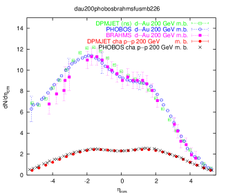
Figure 3: Pseudorapidity distribution of charged hadrons produced in minimum bias $\sqrt{s}=200$ GeV d–Au and p–p collisions. The results of Dpmjet are compared to experimental data from the BRAHMS–Collaboration and the PHOBOS–Collaboration. At some pseudorapidity values the systematic PHOBOS–errors are given.

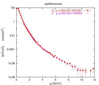
Figure 4: Transverse momentum distribution as measured in p–p collisions at $\sqrt{s}$ = 200 GeV by the PHENIX collaboration at RHIC compared to the calculation by phojet

For other comparisons DPMJET needs some modifications to get agreement with the RHIC data. One of the most important modification is the Percolation of hadronic strings in Dpmjet–III

Using the original Dpmjet–III with enhanced baryon stopping and a centrality of 0 to 5 % the DPMJET multiplicities are larger than the ones measured in Au–Au collisions at RHIC. A new mechanism needed to reduce $N_{ch}$ and $dN_{ch}/d\eta|_{\eta=0}$ in situations with a produced very dense hadronic system. We consider only the percolation and fusion of soft chains (the transverse momenta of both chain ends are below a cut–off $p_{\perp}^{fusion}$ = 2 GeV/c). The condition of percolation is, that the chains overlap in transverse space. We calculate the transverse distance of the chains L and K $R_{L-K}$ and allow fusion of the chains for $R_{L-K}\leq R^{fusion}$ = 0.75 fm. The chains in Dpmjet are fragmented using the Lund code. Only the fragmentation of color triplet–antitriplet chains is available in Jetset, however fusing two arbitrary chains could result in chains with other colors. Therefore, we select only chains for fusion, which again result in triplet–antitriplet chains. Examples are:

(i)A $q_{1}-\bar{q}_{2}$ plus a $q_{3}-\bar{q}_{4}$ chain become a $q_{1}q_{3}-\bar{q}_{2}\bar{q}_{4}$ chain.

(ii)A $q_{1}-q_{2}q_{3}$ plus a $q_{4}-\bar{q}_{2}$ chain become a $q_{1}q_{4}-q_{3}$ chain.

(iii)A $q_{3}-q_{1}q_{2}$ plus a $q_{4}-\bar{q}_{1}$ plus a $\bar{q}_{3}-q_{5}$ chain become a $q_{4}-q_{2}q_{5}$ chain.

(iv)A $q_{4}-\bar{q}_{1}$ plus a $q_{5}-\bar{q}_{3}$ plus a $\bar{q}_{5}-q_{1}$ chain become a $q_{4}-\bar{q}_{3}$ chain.

The expected results of these transformations are a decrease of the number of chains. Even when the fused chains have a higher energy than the original chains, the result will be a decrease of the hadron multiplicity $N_{hadrons}$. In reaction (i) we observe new diquark and anti–diquark chain ends. In the fragmentation of these chains we expect baryon–antibaryon production anywhere in the rapidity region of the collision. Therefore, (i) helps to shift the antibaryon to baryon ratio of the model into the direction as observed in the RHIC experiments.

In Fig.5 we compare the pseudorapidity distributions in Au–Au collisions at 200*A GeV as measured by the PHOBOS collaboration at RHIC for different centralities with the DPMJET–III results obtained with the model including chain percolation and fusion.

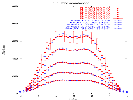
Figure 5: Pseudorapidity distributions of charged hadrons in Au–Au collisions at $\sqrt{(}s)$= 200 GeV for centralities 0–5 % up to 40–50 %. The points with rather small error bars are from the Dpmjet–III Monte Carlo with chain fusion as described in the text. The data points are from the PHOBOS Collaboration.

Further RHIC related improvements (not treated here because of the limited space) in DPMJET include:

(i) Modified $p_{\perp}$ distributions in PYTHIA: For the fragmentation of soft chains the Gaussian transverse momentum distributions in PYTHIA have to be replaced by exponential ones.

(ii) Collision scaling in h–A collisions: To obtain collision scaling in DPMJET we have to change the sampling of hard chains.

(iii) Anomalous baryon stopping: New diagrams lead to more baryons in central region.

(iv) Modified diquark fragmentation: Find missing diagram in diquark fragmentation, to get Antihyperon to Hyperon ratios into agreement with experiment.

3 Model comparisons

This section is based on a talk of D.Heck, Karlsruhe: Comparison of models in the CORSIKA Cosmic Ray cascade code at the VIHKOS CORSIKA School 2005, Lauterbad, Germany, May 31 – June 5, 2005 and Dieter Heck, private communication.

High energy models in CORSIKA used for $E_{lab}\geq$ 80 GeV include: DPMJET 2.55 (J.Ranft,Phys.Rev.D51 (1995) 64), NEXUS 2/3 (J.Drescher et al., Phys.Rep.350 (2001) 93), QGSJET 01/II/III ( S.Ostapchenko, Nucl.Phys.B(Proc.Suppl.)2005), SIBYLL 2.1 (R.Engel et al.,Proc.26${}^{th}$ ICRC 1(1999)415) .

Low energy models in CORSIKA used for $E_{lab}\leq$ 80 GeV include: FLUKA 2003 (only hadron production model) (A.Fasso et al.,Proc.Monte Carlo 2000 (2001)955), GHEISHA 2002 (H.Fesefeld, PITHA–85/02 Aachen (1985)), UrQMD 1.3 (S.A.Bass et al.,Prog.Part.Nucl.Phys.41 (1998)225).

In Fig.6 we compare the average charged multiplicity in p–p collisions as function of the energy between the high energy models. Only the three QGSJET models differ strongly from the rest, at high energies the multiplicity increases much stronger than in the other models. This is the result of the energy independent $p_{\perp}$ cut–off. In Fig.7 we compare the $X_{max}$ of proton and iron induced vertical showers according to the high energy models with $X_{max}$ data. Such a comparison is hoped to determine finally the composition of the highest energy particles in the cosmic radiation. Even, when the models differ considerably like in Fig.6 in their properties, we find here only modest differences in the $X_{max}$ predictions.

In Table 1 we compare the CPU times of the high energy and low energy models. We find only NEXUS and UrQMD to need much more running time than the other models.

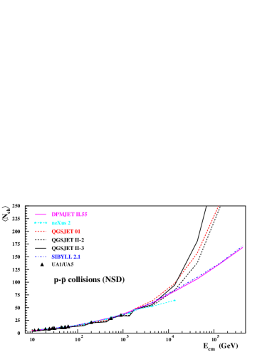
Figure 6: Table 1 Charged particle average multiplicity in $p$–$\bar{p}$ collisions.

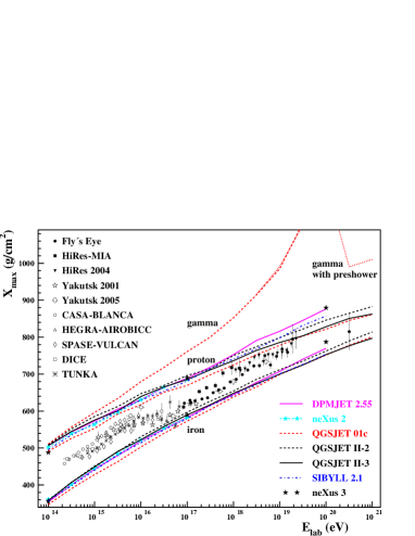
Figure 7: Penetration depth $X_{max}$ for gamma, proton and iron induced vertical showers as function of the energy.

 low energy model   100000 p-Air coll 10 GeV  high energy model   10000 p-Air coll 1 PeV      FLUKA   181 DPMJET 2.55 271   GHEISHA 2002 108 NEXUS 2 3145   UrQMD 1.3 12200 QGSJET II 693   SIBYLL 2.1