Supersymmetric And Smooth Hybrid Inflation
In The Light Of WMAP3

Abstract

In their minimal form both supersymmetric and smooth hybrid inflation yield a scalar spectral index $n_{s}$ close to 0.98, to be contrasted with the result $n_{s}=0.951_{-0.019}^{+0.015}$ from WMAP3. To realize better agreement, following Ref. Bastero-Gil et al. (2006), we extend the parameter space of these models by employing a non-minimal Kähler potential. We also discuss non-thermal leptogenesis by inflaton decay and obtain new bounds in these models on the reheat temperature to explain the observed baryon asymmetry.

I Introduction

Supersymmetric (SUSY) hybrid inflation models Dvali et al. (1994); Lazarides (2002), through their connection to the grand unification scale, provide a compelling framework for the understanding of the early universe. SUSY hybrid inflation is defined by the superpotential $W$ Copeland et al. (1994); Dvali et al. (1994)

$$W=\kappa\widehat{S}(\widehat{\Phi}\widehat{\overline{\Phi}}-M^{2})\,,$$ (1)

where $\widehat{S}$ is a gauge singlet and $\widehat{\Phi}$, $\ \widehat{\overline{\Phi}}$ are a conjugate pair of superfields transforming as nontrivial representations of some group $G$. A simple example of the gauge group $G$ can be provided by the standard model gauge group supplemented by a gauged $U(1)_{B-L}$, which requires, from the anomaly cancellations, the presence of three right handed neutrinos. The Kähler potential can be expanded as

$$K=\left|S\right|^{2}+\left|\Phi\right|^{2}+\left|\overline{\Phi}\right|^{2}+\kappa_{S}\frac{\left|S\right|^{4}}{4m_{p}^{2}}+\cdots$$ (2)

where $S,$ $\Phi$ and $\overline{\Phi}$ are the bosonic components of the superfields, and $m_{p}=2.4\times 10^{18}$ GeV is the reduced Planck mass.

In these models, if the Kähler potential is assumed to be minimal, the scalar spectral index $n_{s}\approx 0.985$ for the dimensionless coupling $\kappa$ in the superpotential $\sim 10^{-2}$, and larger for other values of $\kappa$. The running of the spectral index ${\rm d}n_{s}/{\rm d}\ln k$ and the tensor to scalar ratio $r$ is negligible Şeno$\breve{\textrm{g}}$uz and Shafi (2003, 2005); Jeannerot and Postma (2005). On the other hand, for negligible $r$ the WMAP three year central value for the spectral index is $n_{s}\approx 0.95$, and SUSY hybrid inflation with a minimal Kähler potential is disfavoured at a $2\sigma$ level Spergel et al. (2006).

It was recently shown that the spectral index for SUSY hybrid inflation can be substantially modified in the presence of a small negative mass term in the potential. This can result from a non-minimal Kähler potential, in particular from the term proportional to the dimensionless coupling $\kappa_{S}$ above Bastero-Gil et al. (2006). Ref. Bastero-Gil et al. (2006) presents the results for $\kappa$ values $\gtrsim 10^{-3}$. In this paper we will explore the possible extension of the range of $\kappa$ to lower values depending on $\kappa_{S}$. As we will see increasing the value of $\kappa_{S}$ increases the range of $\kappa$ to lower values, consistent with the measured value of the curvature perturbation amplitude $\mathcal{R}=4.86\times 10^{-5}$. This in turn extends the range of other parameters like the symmetry breaking scale $M$, the inflaton mass $m_{\rm inf}$ and the reheat temperature $T_{r}$.

The outline of the paper is as follows. In section II we consider SUSY hybrid inflation with a non-minimal Kähler potential. Using the standard constraints, we present our numerical results for the allowed range of $\kappa$, $n_{s}$ and $M$ for different values of $\kappa_{S}$. In section III we consider smooth hybrid inflation, an extension of SUSY hybrid inflation which evades potential problems associated with topological defects. We again present how the parameters change with $\kappa_{S}$. In section IV we discuss non-thermal leptogenesis by inflaton decay and show that enough matter asymmetry can be generated with lower values of reheat temperature for nonzero $\kappa_{S}$ in both SUSY and smooth hybrid inflation. We then conclude by reviewing our results in section V.

II SUSY hybrid inflation with non-minimal Kähler potential

Non-minimal supersymmetric hybrid inflation may be defined by the superpotential given in Eq. (1), together with a general Kähler potential

$$K=\left|S\right|^{2}+\left|\Phi\right|^{2}+\left|\overline{\Phi}\right|^{2}+\kappa_{S}\frac{\left|S\right|^{4}}{4m_{p}^{2}}+\kappa_{S\phi}\frac{\left|S\right|^{2}\left|\Phi\right|^{2}}{m_{p}^{2}}+\kappa_{S\overline{\phi}}\frac{\left|S\right|^{2}\left|\overline{\Phi}\right|^{2}}{m_{p}^{2}}+\kappa_{SS}\frac{\left|S\right|^{6}}{6m_{p}^{4}}+\cdots$$ (3)

The SUGRA scalar potential is given by

$$V_{F}=e^{K/m_{p}^{2}}\left(K_{ij}^{-1}D_{z_{i}}WD_{z^{*}_{j}}W^{*}-3m_{p}^{-2}\left|W\right|^{2}\right)$$ (4)

with $z_{i}$ being the bosonic components of the superfields $\widehat{z}_{i}\in\{\widehat{\phi},\widehat{S},\cdots\}$ and where we have defined

$$D_{z_{i}}W \equiv \frac{\partial W}{\partial z_{i}}+m_{p}^{-2}\frac{\partial K}{\partial z_{i}}W$$

$$K_{ij} \equiv \frac{\partial^{2}K}{\partial z_{i}\partial z_{j}^{*}}$$

and $D_{z_{i}^{*}}W^{*}=\left(D_{z_{i}}W\right)^{*}.$ In the D-flat direction $|\Phi|=|\overline{\Phi}|$, and using Eqs. (1, 3) in Eq. (4), we get Panagiotakopoulos (1997a); Asaka et al. (2000)

$$V_{F}=\kappa^{2}M^{4}\left(1-\kappa_{S}\frac{\left|S\right|^{2}}{m_{p}^{2}}+\gamma_{S}\frac{\left|S\right|^{4}}{2m_{p}^{4}}+\cdot\cdot\cdot\right)+\kappa^{2}\left|\Phi\right|^{2}\left(2\left(\left|S\right|^{2}-M^{2}\right)+\cdots\right)+\cdots$$

where $\gamma_{S}=1-\frac{7\kappa_{S}}{2}+2\kappa_{S}^{2}-3\kappa_{SS}.$

In the following discussion and calculations, we will set all the couplings in the Kähler potential except $\kappa_{S}$ to zero. The only coupling except $\kappa_{S}$ which could have a significant effect is $\kappa_{SS}$, since if $\kappa_{SS}$ is large and positive the quartic term becomes negative. The potential in this case is lifted by a higher order term for large values of $\kappa$.

Assuming suitable initial conditions the fields get trapped in the inflationary valley of local minima at $\left|S\right|>S_{c}=M$ and $\left|\Phi\right|=\left|\overline{\Phi}\right|=0$, where $G$ is unbroken. The potential is dominated by the constant term $V_{0}=\kappa^{2}M^{4}$. Inflation ends when the inflaton drops below its critical value $S_{c}=M$ and the fields roll towards the global SUSY minimum of the potential $\left|S\right|=0$ and $\left|\Phi\right|=\left|\overline{\Phi}\right|=M$. In the inflationary trajectory the potential is

$$V_{F}=\kappa^{2}M^{4}\left(1-\kappa_{S}\frac{\left|S\right|^{2}}{m_{p}^{2}}+\gamma_{S}\frac{\left|S\right|^{4}}{2m_{p}^{4}}+\cdots\right)\,.$$

Taking also into account the radiative correction Dvali et al. (1994) and soft SUSY breaking terms, the potential is of the following form

$$V \approx V_{F}+\Delta V_{1loop}+V_{soft}$$ (5)

$$= \kappa^{2}M^{4}\left(1-\kappa_{S}\left(\frac{M}{m_{p}}\right)^{2}x^{2}+\gamma_{S}\left(\frac{M}{m_{p}}\right)^{4}\frac{x^{4}}{2}+\frac{\kappa^{2}\mathcal{N}}{8\pi^{2}}F\right)+a\kappa M^{3}x+a^{2}M^{2}x^{2}$$ (6)

where

$$\Delta V_{1loop}=\frac{1}{64\pi^{2}}Str[{\cal M}^{4}(S)(\ln\frac{{\cal M}^{2}(S)}{Q^{2}}-\frac{3}{2})]=\frac{\left(\kappa M\right)^{4}}{8\pi^{2}}\mathcal{N}F(x)$$

and

$$V_{soft}=a\kappa M^{3}x+a^{2}M^{2}x^{2}$$

with

$$F(x)=\frac{1}{4}\left(\left(x^{4}+1\right)\ln\frac{\left(x^{4}-1\right)}{x^{4}}+2x^{2}\ln\frac{x^{2}+1}{x^{2}-1}+2\ln\frac{\kappa^{2}M^{2}x^{2}}{Q^{2}}-3\right)$$ (7)

and

$$a=m_{3/2}2\left|2-A\right|\cos[\arg S+\arg(2-A)].$$ (8)

Here $\mathcal{N}$ is the dimensionality of the representation of the fields $\Phi$ and $\overline{\Phi},$ $Q$ the renormalization scale and $x=\left|S\right|/M.$ In our numerical calculations we will take $a=1$ TeV.

The number of $e$-folds after the comoving scale $l$ has crossed the horizon is given by

$$N_{l}=2\left(\frac{M}{m_{p}}\right)^{2}\int_{1}^{x_{l}}\left(\frac{V}{\partial_{x}V}\right)dx$$ (9)

where $|S_{l}|=x_{l}M$ is the value of the field at the comoving scale $l$. During inflation, the comoving scale corresponding to $k_{0}=0.002$ Mpc^-1 exits the horizon at approximately

$$N_{0}=53+\frac{1}{3}\ln\left(\frac{T_{r}}{10^{9}~{}{\rm GeV}}\right)+\frac{2}{3}\ln\left(\frac{\sqrt{\kappa}M}{10^{15}~{}{\rm GeV}}\right)$$ (10)

where $T_{r}$ is the reheating temperature, and the subscript ‘0’ indicates that the values are taken at $k_{0}$.

The amplitude of the curvature perturbation is given by

$$\mathcal{R}=\frac{M}{\sqrt{6}\pi m_{p}^{3}}\left(\frac{V^{3/2}}{\partial_{x}V}\right)_{x=x_{0}}=4.86\times 10^{-5}$$ (11)

which is the WMAP normalization at $k_{0}$ Spergel et al. (2006).

Figure 1: The region in the $\kappa$ and $\kappa_{S}$ plane satisfying $\mathcal{R}=4.86\times 10^{-5}$.

For small values of $\kappa,$ $x_{0}$ becomes practically equal to $1$ and the radiative term becomes negligible. The soft mass term $a^{2}M^{2}x^{2}$ is likewise negligible. Eq. (11) then yields

$$\mathcal{R}=\frac{\kappa^{2}}{\sqrt{6}\pi}\left(\frac{M}{m_{p}}\right)^{4}\left(\frac{1}{2\kappa\gamma_{S}\left(\frac{M}{m_{p}}\right)^{5}-2\kappa\kappa_{S}\left(\frac{M}{m_{p}}\right)^{3}+\frac{a}{m_{p}}}\right).$$ (12)

Maximizing this expression with respect to $M$ gives us the lower bound on $\kappa$ from $\mathcal{R}_{\max}=4.86\times 10^{-5}.$ For small values of $\kappa_{S}$ the quartic term is dominant over the quadratic term and these terms become equal for $\kappa_{S}\sim 2\times 10^{-4}.$ For greater values of $\kappa_{S}$ the quadratic term becomes dominant. Numerically, we obtain the lower bounds on $\kappa$ as shown in Fig. 1, with

$$\kappa \gtrsim c_{1}^{5/6}\left(1-c_{1}^{1/3}c_{2}\right)^{5/6}\text{for }\kappa_{S}<6\times 10^{-5}\,,$$

$$\kappa \gtrsim \left(\frac{1}{c_{2}}\right)^{5/2}\left(1-\frac{1}{c_{2}^{3}c_{1}}\right)^{5/2}\text{for }\kappa_{S}>6\times 10^{-5}\,,$$

$$\kappa \gtrsim 9.1\times 10^{-6}\text{ for }\kappa_{S}\sim 6\times 10^{-5}\,,$$

$$\text{where }c_{1} = \frac{5b\sqrt{6}\pi\mathcal{R}_{\max}}{\left(\frac{2b}{\gamma_{S}}\right)^{4/5}}\text{ , }c_{2}=\frac{4\kappa_{S}}{5b}\left(\frac{2b}{\gamma_{S}}\right)^{3/5}\text{ and }b=\frac{a}{m_{p}}\,.$$

For values of $\kappa$ and $M$ such that we can ignore both the quartic and the loop terms in the potential, $\mathcal{R}$ becomes

$$\mathcal{R}\approx\frac{\kappa^{2}}{\sqrt{6}\pi}\left(\frac{M}{m_{p}}\right)^{4}\left(\frac{1}{-2\kappa\kappa_{S}\left(\frac{M}{m_{p}}\right)^{3}+\frac{a}{m_{p}}}\right)\,,$$ (13)

which for $\kappa_{S}>0$ gives the expression for $M$:

$$M\approx\left(\frac{b}{2\kappa\kappa_{S}}\right)^{1/3}\left(1-\frac{\kappa^{2}}{b\sqrt{6}\pi\mathcal{R}}\left(\frac{b}{2\kappa\kappa_{S}}\right)^{4/3}\right)^{1/3}m_{p}\,.$$

Maximizing Eq. (12) with respect to $M$, we find $M=(2b/\kappa\gamma_{S})^{1/5}m_{p}$ at the lower bound on $\kappa$. The numerical values of $M$ obtained using Eqs. (5–10) is shown in Fig. 2.

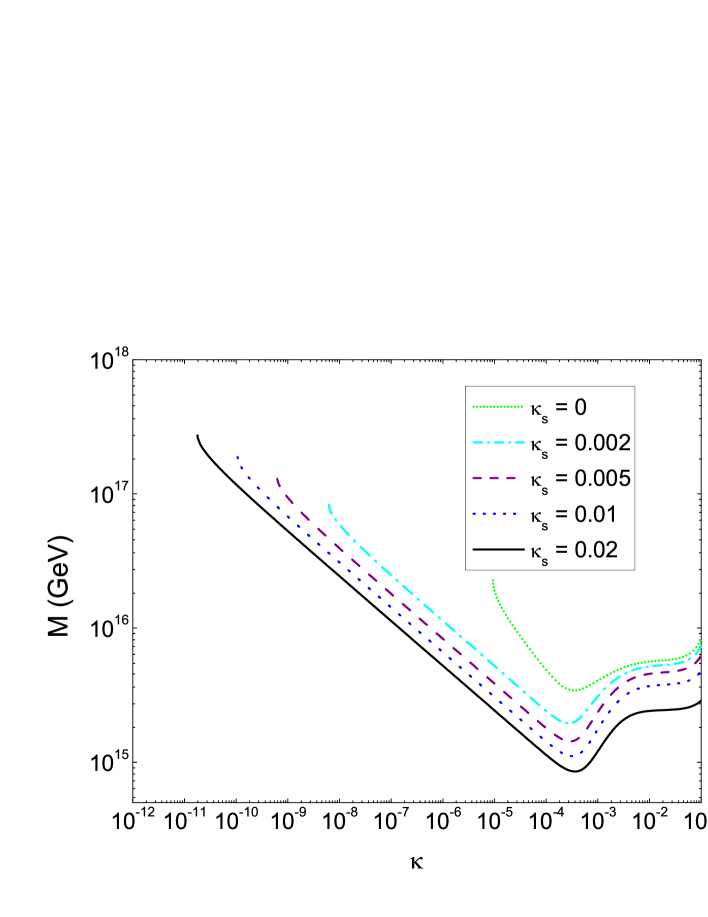
Figure 2: $M$ as a function of $\kappa$ for different values of $\kappa_{S}$ ($\mathcal{N}=1$).

The slow-roll parameters may be defined as

$$\epsilon=\frac{m_{p}^{2}}{2}\left(\frac{V^{\prime}}{V}\right)^{2}\,,\quad\eta=m_{p}^{2}\left(\frac{V^{\prime\prime}}{V}\right)\,,\quad\xi^{2}=m_{p}^{4}\left(\frac{V^{\prime}V^{\prime\prime\prime}}{V^{2}}\right)\,,$$

where $V^{\prime}$ denotes the derivative with respect to the normalized real field $\sigma\equiv\sqrt{2}Mx$. Assuming the slow-roll approximation is valid (i.e. $\epsilon\ll 1,\eta\ll 1$), the spectral index $n_{s}$ and the running of the spectral index ${\rm d}n_{s}/{\rm d}\ln k$ are given by

$$n_{s} \approx 1-6\epsilon+2\eta\,,$$ (14)

$$\frac{dn_{s}}{d\ln k} \approx 16\epsilon\eta-24\epsilon^{2}-2\xi^{2}\,.$$ (15)

Using Eq. (14), we calculate $n_{s}$ as a function of $\kappa$ for different values of $\kappa_{S}$ (Fig. 3). In the $\kappa$ range where the quartic and loop terms are subdominant, from Eq. (13) $n_{s}$ is approximated to be

$$n_{S}=1-2\kappa_{S}+6\gamma_{S}\left(\frac{M}{m_{p}}\right)^{2}x_{0}^{2}+\left(\frac{m_{p}}{M}\right)^{2}\left(\frac{\kappa^{2}\mathcal{N}}{8\pi^{2}}\right)\left.\partial_{x}^{2}F\right|_{x=x_{0}}\simeq 1-2\kappa_{S}\,.$$

This range is represented by the horizontal sections in Fig. 3. For still smaller values of $\kappa$, the quartic term becomes important and the curves bend upward, with $n_{s}$ becoming greater than $1$. We also plot $n_{s}$ versus $\log[V^{1/4}{\rm GeV}]$ and $n_{s}$ for different values of ${\cal N}$ in Figs. 4, 5. The running of the spectral index is negligible in SUSY hybrid inflation, with $|{\rm d}n_{s}/{\rm d}\ln k|\lesssim 10^{-3}$.

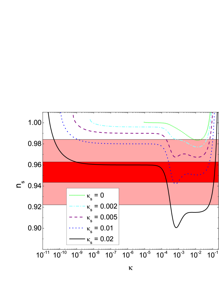
Figure 3: $n_{s}$ as a function of $\kappa$ for different values of $\kappa_{S}$ ($\mathcal{N}=1$). The red and pink bands correspond to the WMAP $1\sigma$ and 2$\sigma$ range Spergel et al. (2006).

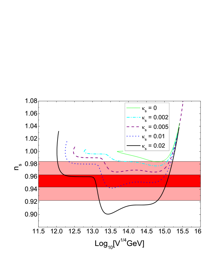
Figure 4: $n_{s}$ as a function of $\log[V^{1/4}{\rm GeV}]$ for different values of $\kappa_{S}$ ($\mathcal{N}=1$). The red and pink bands correspond to the WMAP $1\sigma$ and 2$\sigma$ range Spergel et al. (2006).

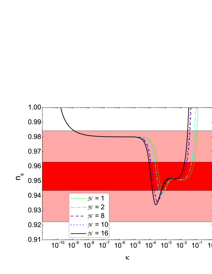
Figure 5: $n_{s}$ as a function of $\kappa$ for different values of $\mathcal{N}$ ($\kappa_{S}=0.01$). The red and pink bands correspond to the WMAP $1\sigma$ and 2$\sigma$ range Spergel et al. (2006).

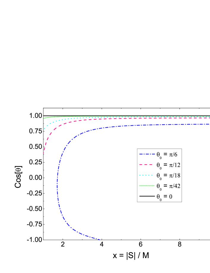
Figure 6: An example to show that the change in $\theta\equiv$ $\arg S$ can be controlled by taking suitable initial conditions, $\theta=\theta_{0}$ and $x=10x_{0}$ ($\arg(2-A)=0$, $\kappa=10^{-4}$, $\kappa_{S}=0$).

It should be noted that for large enough values of $\kappa_{S}$ or small enough values of $\kappa$, the potential develops a false minimum at $\sigma>\sigma_{0}$. Successful inflation then requires the $\sigma$ field to have just enough kinetic energy so that it reaches the local maximum of the potential with negligible kinetic energy. This seems rather improbable since it is realized only for a very narrow band of initial values. Furthermore, we assume that the $A$-term ($a\kappa M^{3}x$) in the potential is positive. Since this depends on the value of $\theta\equiv{\rm arg}S$, it should be checked whether the change in $\theta$ is small. As displayed in Fig. 6, this is possible but again requires specific initial conditions.

Here some discussion of initial conditions is in order. The initial values of the fields can vary in different regions of the universe. Furthermore, the couplings in the Kähler potential are determined by the vacuum expectation values (VEVs) of moduli fields, which can also vary in different regions. The regions with VEVs such that the inflaton mass is suppressed will inflate more and become exponentially large compared to other regions. In this sense, for negative values of $\kappa_{S}$ so that the potential has a positive (mass)² term, the smallness of $|\kappa_{S}|$ ($\kappa_{S}\ll 1$) can be regarded as a selection effect (see Ref. Ross and Sarkar (1996) for a discussion).

However, for positive values of $\kappa_{S}$ the potential has a negative (mass)² term which can lead to a local maximum. Once the inflaton field is sufficiently close to this local maximum (with negligible kinetic energy), eternal inflation is realized. It would then seem that the regions satisfying the conditions for eternal inflation would always dominate, since even if they are initially rare, their volume will increase indefinitely Vilenkin (1983). It is, however, also possible that there are no regions satisfying these conditions. Alternatively, eternal inflation could occur not only close to the local maximum mentioned above, but also at higher energies regardless of the value of $\kappa_{S}$. It then becomes notoriously difficult, if not impossible, to compute the probability distribution of observables such as $n_{s}$, even if the initial distribution of $\kappa_{S}$ is assumed to be known.

To summarize, it is not clear whether the parameter range explored in this paper is less likely to be observed compared to the minimal Kähler potential or negative $\kappa_{S}$ cases. Even if we only consider $\kappa_{S}$ small enough so that the potential remains monotonic, $n_{s}$ can still be significantly lower compared to the minimal Kähler case for large values of $\kappa$, with $n_{s}\simeq 0.95$ for $\kappa\gtrsim 0.1$ and $\kappa_{S}\simeq\kappa/9$.

Finally, we note that for SUSY hybrid inflation there are additional constraints if the symmetry breaking pattern produces cosmic strings Jeannerot and Postma (2005). For example, strings are produced when $\Phi,\,\overline{\Phi}$ break $U(1)_{R}\times U(1)_{B-L}$ to $U(1)_{Y}\times Z_{2}$ matter parity, but not when $\Phi,\,\overline{\Phi}$ are $SU(2)_{R}\times U(1)_{B-L}$ doublets. In this section we assumed that cosmic strings are not produced.

III Smooth hybrid inflation

A variation on SUSY hybrid inflation is obtained by imposing a $Z_{2}$ symmetry on the superpotential, so that only even powers of the combination $\Phi\overline{\Phi}$ are allowed Lazarides and Panagiotakopoulos (1995); Şeno$\breve{\textrm{g}}$uz and Shafi (2005):

$$W=S\left(-v^{2}+\frac{(\Phi\overline{\Phi})^{2}}{M^{2}_{*}}\right)\,,$$ (16)

where the dimensionless parameter $\kappa$ is absorbed in $v$. The resulting scalar potential possesses two (symmetric) valleys of local minima which are suitable for inflation and along which the GUT symmetry is broken. The inclination of these valleys is already non-zero at the classical level and the end of inflation is smooth, in contrast to SUSY hybrid inflation. An important consequence is that potential problems associated with topological defects are avoided. This ‘smooth hybrid inflation’ model is similar to the ‘mutated hybrid inflation’ model considered in Ref. Stewart (1995) and generalized in Ref. Lyth and Stewart (1996).

The common VEV at the SUSY minimum $M=\big{|}\langle\nu^{c}_{H}\rangle\big{|}=\big{|}\langle\overline{\nu}^{c}_{H}\rangle\big{|}=(v\,M_{*})^{1/2}$. For $\sigma^{2}\gg M^{2}$, the inflationary potential is given by

$$V\approx v^{4}\left[1-\frac{2}{27}\frac{M^{4}}{\sigma^{4}}+\frac{\sigma^{4}}{8m^{4}_{p}}\right]\,,$$ (17)

where the last term arises from the SUGRA correction for a minimal Kähler potential Şeno$\breve{\textrm{g}}$uz and Shafi (2005). The soft terms in this case do not have a significant effect on the inflationary dynamics. If we set $M$ equal to the SUSY GUT scale $M_{\rm GUT}=2\times 10^{16}$ GeV, we get $v\approx 1.4\times 10^{15}$ GeV and $M_{*}\approx 2.8\times 10^{17}$ GeV. (Note that, if we express Eq. (16) in terms of the coupling parameter $\kappa$, this value corresponds to $\kappa\sim O(v^{2}/M^{2}_{\rm GUT})\sim 10^{-2}$.) The value of the field $\sigma$ is $1.1\times 10^{17}$ GeV at the end of inflation (corresponding to $\eta=-1$) and $\sigma_{0}\approx 2.4\times 10^{17}$ GeV at $k_{0}$. In the absence of the SUGRA correction (which is small for $M\lesssim 10^{16}$ GeV), $\sigma_{0}\propto M^{2/3}\,m_{p}^{1/3}$, $\mathcal{R}\propto M^{10/3}/(M^{2}_{*}\,m_{p}^{4/3})$ and the spectral index is given by Lazarides and Panagiotakopoulos (1995)

$$n_{s}\approx 1-\frac{5}{3N_{0}}\approx 0.97\,.$$ (18)

The SUGRA correction raises $n_{s}$ from 0.97 to above unity for $M\gtrsim 1.5\times 10^{16}$ GeV Şeno$\breve{\textrm{g}}$uz and Shafi (2005).

One problem with this model is that the cutoff scale $M_{*}$ is close to the inflaton field value $\sigma_{0}$ for $M\simeq M_{\rm GUT}$. $M_{*}$ becomes smaller than $\sigma_{0}$ for $M\lesssim 10^{16}$ GeV, for which the effective field theory is in general no longer valid. However, with a negative mass term that could result from a non-minimal Kähler potential larger values of $M_{*}$ are possible. Also, as in SUSY hybrid inflation, the spectral index can have lower values.

For a Kähler potential $K=|S|^{2}+|\Phi|^{2}+|\overline{\Phi}|^{2}+\lambda|S|^{4}/4M^{2}_{*}+\ldots$, the potential is obtained as

$$V\approx v^{4}\left[1-\frac{2}{27}\frac{M^{4}}{\sigma^{4}}-\frac{\kappa_{S}}{2}\frac{\sigma^{2}}{m^{2}_{p}}+\frac{\gamma_{S}}{8}\frac{\sigma^{4}}{m^{4}_{p}}\right]\,.$$ (19)

Here we have defined $\kappa_{S}\equiv\lambda m_{p}^{2}/M^{2}_{*}$ to express the potential in a form similar to that of the previous section. The $M_{*}$ and $\sigma_{0}$ values for different values of $\kappa_{S}$ is displayed in Fig. 7.

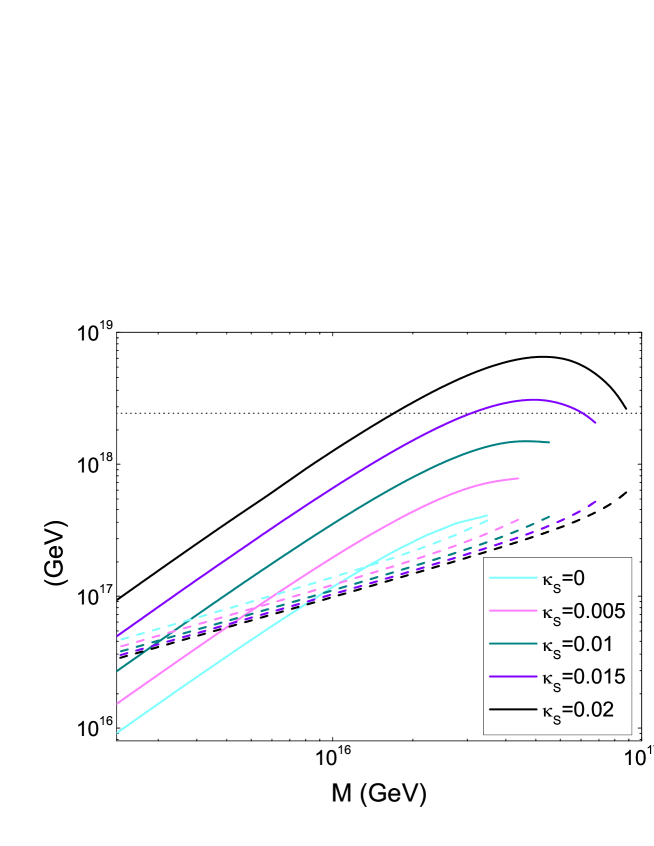
Figure 7: $M_{*}$ (solid) and $\sigma_{0}$ (dashed) as functions of the gauge symmetry breaking scale $M$ for smooth hybrid inflation.

The spectral index $n_{s}$ for different values of $\kappa_{S}$ is displayed in Fig. 8. Note that for $\kappa_{S}=0$, requiring $\sigma_{0}<M_{*}$ constrains $n_{s}\gtrsim 0.99$. Having a non-zero $\kappa_{S}$ allows smaller values of $n_{s}$ in better agreement with the WMAP3 results. For large enough values of $\kappa_{S}$ or small enough values of $M$ (the dashed sections in the figure), the potential develops a false minimum at $\sigma>\sigma_{0}$ as in SUSY hybrid inflation. Again, even with $|\kappa_{S}|$ small enough so that there is no such false minimum, $n_{s}$ can be as low as $0.95$.

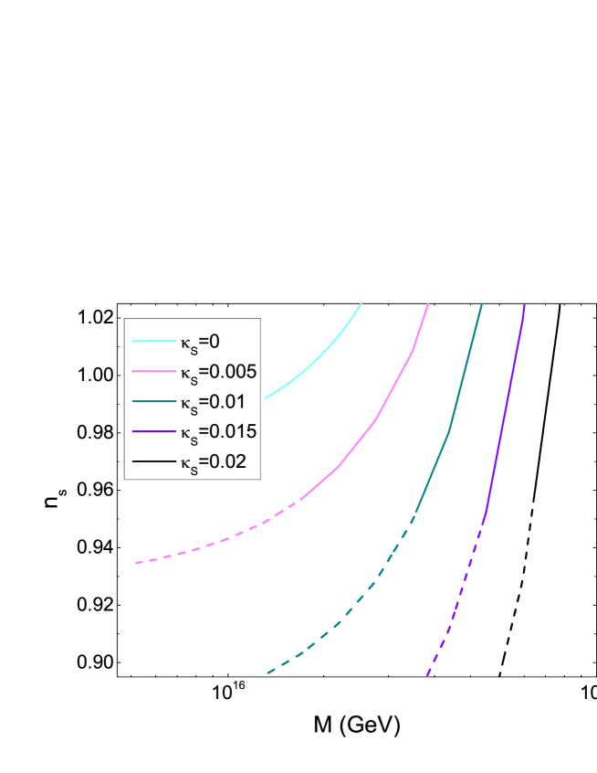
Figure 8: The spectral index $n_{s}$ as a function of the gauge symmetry breaking scale $M$ for smooth hybrid inflation. The dashed sections indicate that the field is initially close to a local maximum.

IV Reheat temperature and the gravitino constraint

After the end of inflation, the fields fall toward the SUSY vacuum and perform damped oscillations about it. The VEVs of $\Phi$ and $\overline{\Phi}$, along their right handed neutrino components $\nu_{H}^{c}$, $\overline{\nu}_{H}^{c}$, break the gauge symmetry. The oscillating system, which we collectively denote as $\chi$, consists of the two complex scalar fields $\left(\delta\nu_{H}^{c}+\delta\overline{\nu}_{H}^{c}\right)/\sqrt{2}$ (where $\delta\nu_{H}^{c}$, $\delta\overline{\nu}_{H}^{c}$ are the deviations of $\nu_{H}^{c}$, $\overline{\nu}_{H}^{c}$ from $M$) and $S$, with equal mass $m_{\rm inf}$.

We assume here that the inflaton $\chi$ decays predominantly into right handed neutrino superfields $N_{i}$, via the superpotential coupling $(1/m_{P})\gamma_{ij}\overline{\Phi}\Phi N_{i}N_{j}$ or $\gamma_{ij}\overline{\Phi}N_{i}N_{j}$, where $i,j$ are family indices. Their subsequent out of equilibrium decay to lepton and Higgs superfields generates lepton asymmetry, which is then partially converted into the observed baryon asymmetry by sphaleron effects.

The right handed neutrinos, as shown below, can be heavy compared to the reheat temperature $T_{r}$. Note that unlike thermal leptogenesis, there is then no washout factor since lepton number violating 2-body scatterings mediated by right handed neutrinos are out of equilibrium as long as the lightest right handed neutrino mass $M_{1}\gg T_{r}$ Fukugita and Yanagida (1990). More precisely, the washout factor is proportional to $e^{-z}$ where $z=M_{1}/T_{r}$ Buchmuller et al. (2003), and can be neglected for $z\gtrsim 10$. Without this assumption, generating sufficient lepton asymmetry would require $T_{r}\gtrsim 2\times 10^{9}$ GeV Giudice et al. (2004), and as discussed below this is hard to reconcile with the gravitino constraint.

GUTs typically relate the Dirac neutrino masses to that of the quarks or charged leptons. It is therefore reasonable to assume that the Dirac masses are hierarchical. The low-energy neutrino data indicates that the right handed neutrinos in this case will also be hierarchical in general. As discussed in Ref. Akhmedov et al. (2003), setting the Dirac masses strictly equal to the up-type quark masses and fitting to the neutrino oscillation parameters generally yields strongly hierarchical right handed neutrino masses ($M_{1}\ll M_{2}\ll M_{3}$), with $M_{1}$ $\sim 10^{5}$ GeV. The lepton asymmetry in this case is too small by several orders of magnitude. However, it is plausible that there are large radiative corrections to the first two family Dirac masses, so that $M_{1}$ remains heavy compared to $T_{r}$.

A reasonable mass pattern is therefore $M_{1}<M_{2}\ll M_{3}$, which can result from either the dimensionless couplings $\gamma_{ij}$ or additional symmetries. The dominant contribution to the lepton asymmetry is from the decays with $N_{3}$ in the loop, as long as the first two family right handed neutrinos are not quasi-degenerate. Under these assumptions, the lepton asymmetry is given by Asaka et al. (2000); Şeno$\breve{\textrm{g}}$uz and Shafi (2005)

$$n_{L}/s\lesssim 3\times 10^{-10}\frac{T_{r}}{m_{\rm inf}}\left(\frac{M_{i}}{10^{6}{\rm~{}GeV}}\right)\left(\frac{m_{\nu 3}}{0.05{\rm~{}eV}}\right),$$ (20)

where $M_{i}$ denotes the mass of the heaviest right handed neutrino the inflaton can decay into.

From the experimental value of the baryon to photon ratio $\eta_{B}\approx$ $6.1\times 10^{-10}$ Spergel et al. (2006), the required lepton asymmetry is found to be $n_{L}/s\approx 2.5\times 10^{-10}$ Khlebnikov and Shaposhnikov (1988). Since $m_{\rm inf}>2M_{i}$, Eq. (20) then yields

$$T_{r}\gtrsim 1.6\times 10^{6}\ {\rm GeV}\left(\frac{0.05\ {\rm eV}}{m_{\nu 3}}\right)\,.$$ (21)

This is a general bound valid for non-thermal leptogenesis by inflaton decay, assuming hierarchical right handed neutrinos that are heavy compared to $T_{r}$. More specific bounds can be obtained using the inflaton decay rate $\Gamma_{\chi}$ $=(1/8\pi)(M_{i}^{2}/M^{2})m_{\rm inf}$. The reheat temperature $T_{r}$ is given by

$$T_{r}=\left(\frac{45}{2\pi^{2}g_{*}}\right)^{1/4}\left(\Gamma_{\chi}m_{p}\right)^{1/2}\approx 0.063\frac{(m_{p}m_{\rm inf})^{1/2}}{M}M_{i}\,.$$ (22)

For SUSY hybrid inflation the values of $m_{\rm inf}=\sqrt{2}\kappa M$ are shown in Fig. 9. Eq. (22) yields the result that $M_{i}$ is about 200 (6) times heavier than $T_{r}$, for $\kappa=10^{-5}$ ($10^{-2}$) with $\kappa_{S}=0$. $M_{i}/T_{r}$ decreases slightly for non-zero $\kappa_{S}$, with $M_{i}/T_{r}\approx 150$ (5) for the same $\kappa$ values and $\kappa_{S}=0.01$. Thus, small values of $\kappa$ are consistent with ignoring washout effects as long as the lightest right handed neutrino mass $M_{1}$ is also $\gg T_{r}$.

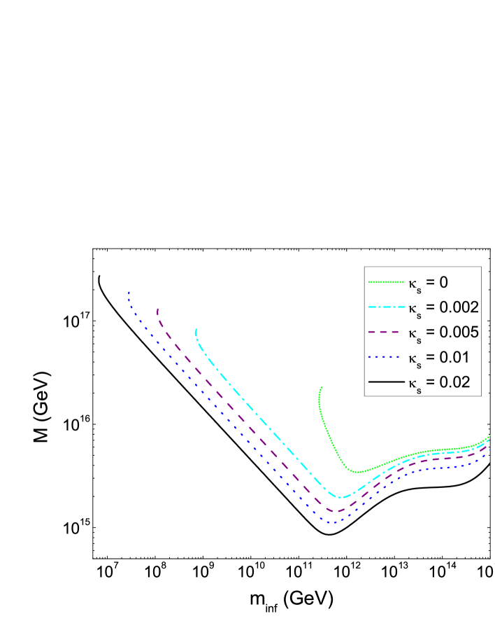
Figure 9: $M$ as a function of $m_{\rm inf}$ for different values of $\kappa_{S}$ ($\mathcal{N}=1$).

Using the required value of $n_{L}/s$ along with Eqs. (20, 22), we can express the $T_{r}$ sufficient to generate the observed matter asymmetry in terms of the symmetry breaking scale $M$ and the inflaton mass $m_{\rm inf}$:

$$T_{r}\gtrsim 1.6\times 10^{7}{\rm\ GeV}\left(\frac{10^{16}{\rm\ GeV}}{M}\right)^{1/2}\left(\frac{m_{\rm inf}}{10^{11}{\rm\ GeV}}\right)^{3/4}\left(\frac{0.05\rm{\ eV}}{m_{\nu 3}}\right)^{1/2}\,.$$ (23)

We show the lower bound on $T_{r}$ calculated using this equation in Fig. 10 (taking $m_{\nu 3}$ $=0.05$ eV). The limit in Eq. (21) is saturated at $\kappa\approx 3\times 10^{-7}$, where $m_{\rm inf}=2M_{i}$. For smaller values of $\kappa$, sufficient lepton asymmetry cannot be obtained unless the asymmetry is enhanced by having quasi-degenerate neutrinos.

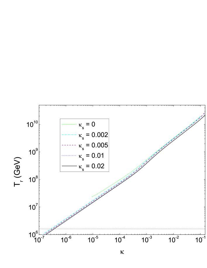
Figure 10: $T_{r}$ as a function of $\kappa$ for different values of $\kappa_{S}$ ($\mathcal{N}=1$).

For smooth hybrid inflation, $m_{\rm inf}$ is given by $2\sqrt{2}v^{2}/M$. The value of $m_{\rm inf}$ is shown in Fig. 11. From Eq. (22), $M_{i}/T_{r}$ is about 10 (40) for $\kappa_{S}=0$ ($0.01$). We show the lower bound on $T_{r}$ (taking $m_{\nu 3}=0.05$ eV) in Fig. 12.

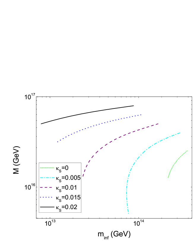
Figure 11: The inflaton mass $m_{\rm inf}$ vs. the symmetry breaking scale $M$ for smooth hybrid inflation. Only those sections satisfying $M_{*}>\sigma_{0}$ and $0.9<n_{s}<1.02$ are shown.

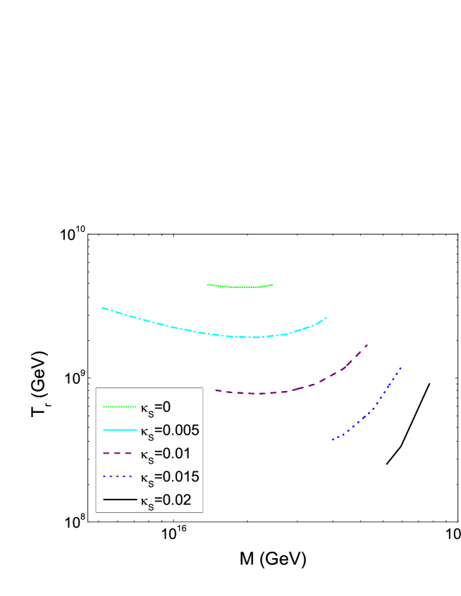
Figure 12: The lower bound on the reheat temperature $T_{r}$ vs. the symmetry breaking scale $M$ for smooth hybrid inflation. Only those sections satisfying $M_{*}>\sigma_{0}$ and $0.9<n_{s}<1.02$ are shown.

An important constraint on supersymmetric inflation models arises from considering the reheat temperature $T_{r}$ after inflation, taking into account the gravitino problem which requires that $T_{r}\lesssim 10^{6}$–$10^{10}$ GeV Khlopov and Linde (1984). This constraint on $T_{r}$ depends on the SUSY breaking mechanism and the gravitino mass $m_{3/2}$. For gravity mediated SUSY breaking models with unstable gravitinos of mass $m_{3/2}\simeq 0.1$–1 TeV, $T_{r}\lesssim 10^{6}$–$10^{9}$ GeV Kawasaki and Moroi (1995), while $T_{r}\lesssim 10^{10}$ GeV for stable gravitinos Bolz et al. (2001). In view of these bounds, smooth hybrid inflation is relatively disfavoured compared to SUSY hybrid inflation since $T_{r}\gtrsim 10^{9}$ for $M=M_{\rm GUT}$.

Besides the thermal production of gravitinos which puts an upper bound on $T_{r}$, there are also constraints from gravitinos directly produced by inflaton decay. It was recently pointed out that these constraints can be rather severe for SUSY and smooth hybrid inflation Kawasaki et al. (2006a), although since the gravitino production depends on the SUSY breaking sector the models are still viable. As displayed in Fig. 9, significantly lower values of $m_{\rm inf}$ can be obtained with a non-minimal Kähler potential for SUSY hybrid inflation. This extends the allowed range of parameters where the gravitino constraint can be evaded. For smooth hybrid inflation $m_{\rm inf}$ tends to be higher (Fig. 11).

Finally we note that our estimates for the reheat temperature and matter asymmetry may be affected due to MSSM flat directions delaying the thermalization of inflaton decay products or dominating the energy density of the Universe Allahverdi:2005fq , although it has been argued that the flat directions can decay rapidly due to non-perturbative effects Olive:2006uw . Also, there can be additional sources of baryon asymmetry such as ‘coherent baryogenesis’ Garbrecht:2003mn .

V Conclusion

We considered supersymmetric hybrid inflation and smooth hybrid inflation models using a general (non-minimal) Kähler potential. The parameter space of the models are extended compared to the minimal Kähler potential case. With a negative mass term in the potential, it is possible to obtain values of the spectral index in the central WMAP3 range. Also, sufficient matter asymmetry can be generated with lower values of the reheat temperature.

In most of the parameter range we consider, the potential develops a false minimum at large field values and successful inflation is then only possible with specific initial conditions. However, since these initial conditions lead to eternal inflation, it is not clear whether this parameter range is less likely to be observed than the minimal Kähler potential case. Even if we only consider the range for which the potential is monotonic, it is still possible to obtain a spectral index as low as 0.95 with a negligible tensor to scalar ratio. For supersymmetric hybrid inflation this requires $\kappa\gtrsim 0.1$ while the gravitino problem favors smaller values of $\kappa$.

References

- Bastero-Gil et al. (2006) M. Bastero-Gil, S. F. King, and Q. Shafi (2006), eprint hep-ph/0604198.
- Dvali et al. (1994) G. R. Dvali, Q. Shafi, and R. K. Schaefer, Phys. Rev. Lett. 73, 1886 (1994), eprint hep-ph/9406319.
- Lazarides (2002) G. Lazarides, Lect. Notes Phys. 592, 351 (2002), eprint hep-ph/0111328.
- Copeland et al. (1994) E. J. Copeland, A. R. Liddle, D. H. Lyth, E. D. Stewart, and D. Wands, Phys. Rev. D49, 6410 (1994), eprint astro-ph/9401011.
- Fayet (1975) P. Fayet, Nucl. Phys. B90, 104 (1975).
- Şenouz and Shafi (2005) V. N. Şenouz and Q. Shafi, Phys. Rev. D71, 043514 (2005), eprint hep-ph/0412102.
- Jeannerot and Postma (2005) R. Jeannerot and M. Postma, JHEP 05, 071 (2005), eprint hep-ph/0503146.
- Şenouz and Shafi (2003) V. N. Şenouz and Q. Shafi, Phys. Lett. B567, 79 (2003), eprint hep-ph/0305089.
- Spergel et al. (2006) D. N. Spergel et al. (2006), eprint astro-ph/0603449.
- (10) W. H. Kinney, E. W. Kolb, A. Melchiorri and A. Riotto, Phys. Rev. D 74, 023502 (2006), eprint astro-ph/0605338.
- Panagiotakopoulos (1997a) C. Panagiotakopoulos, Phys. Rev. D55, 7335 (1997a), eprint hep-ph/9702433; A. D. Linde and A. Riotto, Phys. Rev. D56, 1841 (1997), eprint hep-ph/9703209; C. Panagiotakopoulos, Phys. Lett. B402, 257 (1997b), eprint hep-ph/9703443; G. Lazarides and N. Tetradis, Phys. Rev. D58, 123502 (1998), eprint hep-ph/9802242; W. Buchmuller, L. Covi, and D. Delepine, Phys. Lett. B491, 183 (2000), eprint hep-ph/0006168; M. Kawasaki, M. Yamaguchi, and J. Yokoyama, Phys. Rev. D68, 023508 (2003), eprint hep-ph/0304161.
- Asaka et al. (2000) T. Asaka, K. Hamaguchi, M. Kawasaki, and T. Yanagida, Phys. Rev. D61, 083512 (2000), eprint hep-ph/9907559.
- Ross and Sarkar (1996) G. G. Ross and S. Sarkar, Nucl. Phys. B461, 597 (1996), eprint hep-ph/9506283.
- (14) R. Allahverdi, K. Enqvist, J. Garcia-Bellido and A. Mazumdar, Phys. Rev. Lett. 97, 191304 (2006), eprint hep-ph/0605035; R. Allahverdi, K. Enqvist, J. Garcia-Bellido, A. Jokinen and A. Mazumdar (2006), eprint hep-ph/0610134; J. C. Bueno Sanchez, K. Dimopoulos and D. H. Lyth (2006), eprint hep-ph/0608299.
- Vilenkin (1983) A. Vilenkin, Phys. Rev. D27, 2848 (1983); A. D. Linde, Particle Physics and Inflationary Cosmology (Harwood Academic, 1990), eprint hep-th/0503203; L. Boubekeur and D. H. Lyth, JCAP 0507, 010 (2005), eprint hep-ph/0502047.
- Vilenkin (2006) A. Vilenkin (2006), eprint hep-th/0609193.
- Tegmark (2005) M. Tegmark, JCAP 0504, 001 (2005), eprint astro-ph/0410281.
- Lazarides and Panagiotakopoulos (1995) G. Lazarides and C. Panagiotakopoulos, Phys. Rev. D52, 559 (1995), eprint hep-ph/9506325; G. Lazarides, C. Panagiotakopoulos, and N. D. Vlachos, Phys. Rev. D54, 1369 (1996), eprint hep-ph/9606297; R. Jeannerot, S. Khalil, and G. Lazarides, Phys. Lett. B506, 344 (2001), eprint hep-ph/0103229.
- Stewart (1995) E. D. Stewart, Phys. Lett. B345, 414 (1995), eprint astro-ph/9407040.
- Lyth and Stewart (1996) D. H. Lyth and E. D. Stewart, Phys. Rev. D54, 7186 (1996), eprint hep-ph/9606412.
- Fukugita and Yanagida (1986) M. Fukugita and T. Yanagida, Phys. Lett. B174, 45 (1986).
- Lazarides and Shafi (1991) G. Lazarides and Q. Shafi, Phys. Lett. B258, 305 (1991).
- Lazarides et al. (1997) G. Lazarides, R. K. Schaefer, and Q. Shafi, Phys. Rev. D56, 1324 (1997), eprint hep-ph/9608256.
- Fukugita and Yanagida (1990) M. Fukugita and T. Yanagida, Phys. Rev. D42, 1285 (1990); L. E. Ibanez and F. Quevedo, Phys. Lett. B283, 261 (1992), eprint hep-ph/9204205.
- Buchmuller et al. (2003) W. Buchmuller, P. Di Bari, and M. Plumacher, Nucl. Phys. B665, 445 (2003), eprint hep-ph/0302092.
- Giudice et al. (2004) G. F. Giudice, A. Notari, M. Raidal, A. Riotto, and A. Strumia, Nucl. Phys. B685, 89 (2004), eprint hep-ph/0310123; W. Buchmuller, P. Di Bari, and M. Plumacher, Ann. Phys. 315, 305 (2005), eprint hep-ph/0401240.
- Akhmedov et al. (2003) E. K. Akhmedov, M. Frigerio, and A. Y. Smirnov, JHEP 09, 021 (2003), eprint hep-ph/0305322.
- Khlebnikov and Shaposhnikov (1988) S. Y. Khlebnikov and M. E. Shaposhnikov, Nucl. Phys. B308, 885 (1988).
- Flanz et al. (1996) M. Flanz, E. A. Paschos, U. Sarkar, and J. Weiss, Phys. Lett. B389, 693 (1996), eprint hep-ph/9607310.
- Pilaftsis (1997) A. Pilaftsis, Phys. Rev. D56, 5431 (1997), eprint hep-ph/9707235; A. Pilaftsis and T. E. J. Underwood, Nucl. Phys. B692, 303 (2004), eprint hep-ph/0309342.
- Khlopov and Linde (1984) M. Y. Khlopov and A. D. Linde, Phys. Lett. B138, 265 (1984); J. R. Ellis, J. E. Kim, and D. V. Nanopoulos, Phys. Lett. B145, 181 (1984).
- Kawasaki and Moroi (1995) M. Kawasaki and T. Moroi, Prog. Theor. Phys. 93, 879 (1995), eprint hep-ph/9403364; R. H. Cyburt, J. R. Ellis, B. D. Fields, and K. A. Olive, Phys. Rev. D67, 103521 (2003), eprint astro-ph/0211258; M. Kawasaki, K. Kohri, and T. Moroi (2004), eprint astro-ph/0402490.
- Bolz et al. (2001) M. Bolz, A. Brandenburg, and W. Buchmuller, Nucl. Phys. B606, 518 (2001), eprint hep-ph/0012052; M. Fujii, M. Ibe, and T. Yanagida, Phys. Lett. B579, 6 (2004), eprint hep-ph/0310142; L. Roszkowski, R. Ruiz de Austri, and K.-Y. Choi, JHEP 08, 080 (2005), eprint hep-ph/0408227.
- Şenouz and Shafi (2004) V. N. Şenouz and Q. Shafi, Phys. Lett. B596, 8 (2004), eprint hep-ph/0403294.
- Kawasaki et al. (2006a) M. Kawasaki, F. Takahashi, and T. T. Yanagida, Phys. Lett. B638, 8 (2006a), eprint hep-ph/0603265; T. Asaka, S. Nakamura, and M. Yamaguchi, Phys. Rev. D74, 023520 (2006), eprint hep-ph/0604132; M. Dine, R. Kitano, A. Morisse, and Y. Shirman, Phys. Rev. D73, 123518 (2006), eprint hep-ph/0604140; M. Endo, K. Hamaguchi, and F. Takahashi, Phys. Rev. D74, 023531 (2006a), eprint hep-ph/0605091; M. Kawasaki, F. Takahashi, and T. T. Yanagida, Phys. Rev. D74, 043519 (2006b), eprint hep-ph/0605297; M. Endo, M. Kawasaki, F. Takahashi, and T. T. Yanagida, Phys. Lett. B642, 518 (2006b), eprint hep-ph/0607170.
- (36) R. Allahverdi and A. Mazumdar (2005), eprint hep-ph/0505050; JCAP 0610, 008 (2006), eprint hep-ph/0512227.
- (37) K. A. Olive and M. Peloso, Phys. Rev. D 74, 103514 (2006), eprint hep-ph/0608096.
- (38) B. Garbrecht, T. Prokopec and M. G. Schmidt, Phys. Rev. Lett. 92, 061303 (2004), eprint hep-ph/0304088; eprint hep-ph/0410132; Nucl. Phys. B 736, 133 (2006), eprint hep-ph/0509190.