Nucleon Electromagnetic Form Factors

Abstract

There has been much activity in the measurement of the elastic electromagnetic proton and neutron form factors in the last decade, and the quality of the data has been greatly improved by performing double polarization experiments, in comparison with previous unpolarized data. Here we review the experimental data base in view of the new results for the proton, and neutron, obtained at MIT-Bates, MAMI, and JLab. The rapid evolution of phenomenological models triggered by these high-precision experiments will be discussed, including the recent progress in the determination of the valence quark generalized parton distributions of the nucleon, as well as the steady rate of improvements made in the lattice QCD calculations.

Keywords: Nucleon structure; Elastic electromagnetic form factors

1 Introduction

The characterization of the structure of the nucleon is a defining problem of hadronic physics, much like the hydrogen atom is to atomic physics. Elastic nucleon form factors (FFs) are key ingredients of this characterization. As such, a full and detailed quantitative understanding of the internal structure of the nucleon is a necessary precursor to extending our understanding of hadronic physics.

The electromagnetic (e.m.) interaction provides a unique tool to investigate the internal structure of the nucleon. The measurements of e.m. FFs in elastic as well as inelastic scattering, and the measurements of structure functions in deep inelastic scattering of electrons, have been a rich source of information on the structure of the nucleon.

The investigation of the spatial distributions of the charge and magnetism carried by nuclei started in the early nineteen fifties; it was profoundly affected by the original work of one of its earliest pioneers, Hofstadter and his team of researchers [Hof53b], at the Stanford University High Energy Physics Laboratory. Quite early the interest turned to the nucleon; the first FF measurements of the proton were reported in 1955 [Hof55], and the first measurement of the neutron magnetic FF was reported by Yearian and Hofstadter [Yea58] in 1958. Simultaneously much theoretical work was expanded to the development of models of the nucleus, as well as the interaction of the electromagnetic probe with nuclei and the nucleon. The prevailing model of the proton at the time, was developed by Rosenbluth [Ros50], and consisted of a neutral baryonic core, surrounded by a positively charged pion cloud.

Following the early results obtained at the Stanford University High Energy Physics Laboratory, similar programs started at several new facilities, including the Laboratoire de l’Accélerateur Linéaire in Orsay, (France), the Cambridge Electron Accelerator, the Electron-Synchrotron at Bonn, the Stanford Linear Accelerator Center (SLAC), Deutsches Elektronen-Synchrotron (DESY) in Hamburg, the 300 MeV linear accelerator at Mainz, the electron accelerators at CEA-Saclay, and at Nationaal Instituut voor Kernfysica en Hoge Energie Fysica (NIKHEF). The number of electron accelerators and laboratories, and the beam quality, grew steadily, reflecting the increasing interest of the physics problems investigated and results obtained using electron scattering. The most recent generation of electron accelerators, which combine high current with high polarization electron beams, at MIT-Bates, the Mainz Microtron (MAMI), and the Continuous Electron Beam Accelerator Facility (CEBAF) of the Jefferson Lab (JLab), have made it possible to investigate the internal structure of the nucleon with unprecedented precision. The CEBAF accelerator adds the unique feature of high energy which allows to perform measurements of nucleon e.m. FFs to large momentum transfers. Sizable parts of the programs at these facilities were and are oriented around efforts to characterize the spatial distribution of charge and magnetization in nuclei and in the nucleon.

The recent and unexpected results from JLab of using the polarization transfer technique to measure the proton electric over magnetic FF ratio, $G_{Ep}/G_{Mp}$ [Jon00, Gay02, Pun05], has been the revelation that the FFs obtained using the polarization and Rosenbluth cross section separation methods, were incompatible with each other, starting around $Q^{2}=3$ GeV². The FFs obtained from cross section data had suggested that $G_{Ep}\sim G_{Mp}/\mu_{p}$, where $\mu_{p}$ is the proton magnetic moment; the results obtained from recoil polarization data clearly show that the ratio $G_{Ep}/G_{Mp}$ decreases linearly with increasing momentum transfer $Q^{2}$. The numerous attempts to explain the difference in terms of radiative corrections which affect the results of the Rosenbluth separation method very significantly, but polarization results only minimally, have led to the previously neglected calculation of two hard photon exchange with both photons sharing the momentum transfer.

These striking results for the proton e.m. FF ratio as well as high precision measurements of the neutron electric FF, obtained through double polarization experiments, have put the field of nucleon elastic e.m. FFs into the limelight, giving it a new life. Since the publication of the JLab ratio measurements, there have been two review papers on the subject of nucleon e.m. FFs [Gao03, Hyd04], with a third one just recently completed [Arr06]. The present review complements the previous ones by bringing the experimental situation up-to-date, and gives an overview of the latest theoretical developments to understand the nucleon e.m. FFs from the underlying theory of the strong interactions, Quantum Chromodynamics (QCD). We will focus in this review on the space-like nucleon e.m. FFs, as they have been studied in much more detail both experimentally and theoretically than their time-like counterparts [Bal05]. We will also not discuss the strangeness FFs of the nucleon which have been addressed in recent years through dedicated parity violating electron scattering experiments. For a recent review of the field of parity violating electron scattering and strangeness FFs, see e.g. Ref. [Bei05].

This review is organized as follows. Section 2 is dedicated to a description of the beginning of the field of electron scattering on the nucleon, and the development of the theoretical tools and understanding required to obtain the fundamental FFs. Elastic differential cross section data lend themselves to the separation of the two e.m. FFs of proton and neutron by the Rosenbluth, or LT-separation method. All experimental results obtained in this way are shown and discussed.

Section 3 discusses the development of another method, based on double polarization, either measuring the proton recoil polarization in $\vec{e}p\rightarrow{e}\vec{p}$, or the asymmetry in $\vec{e}\vec{p}\rightarrow{ep}$. The now well documented and abundantly discussed difference in the FF results obtained by Rosenbluth separation on the one hand, and double polarization experiments on the other hand, is examined in section 3.4. The radiative corrections, including two-photon exchange corrections, essential to obtain the Born approximation FFs, are discussed in details in section 3.5.

In Section 4, we present an overview of the theoretical understanding of the nucleon e.m. FFs. In Sect. 4.1, we firstly discuss vector meson dominance models and the latest dispersion relation fits. To arrive at an understanding of the nucleon e.m. FFs in terms of quark and gluon degrees of freedom, we next examine in Sect. 4.2 constituent quark models. We discuss the role of relativity when trying to arrive at a microscopic description of nucleon FFs based on quark degrees of freedom in the few GeV² region. The present limitations in such models will also be addressed. In Sect. 4.3, we highlight the spatial information which can be extracted from the nucleon e.m. FFs, the role of the pion cloud, and the issue of shape of hadrons. Sect. 4.4 discusses the chiral effective field theory of QCD and their predictions for the nucleon e.m. FFs at low momentum transfers. Sect. 4.5 examines the ab initio calculations of nucleon e.m. FFs using lattice QCD. We will compare the most recent results and the open issues in this field. We also explain how the chiral effective field theory can be useful in extrapolating lattice QCD calculations for FFs, performed at larger than physical pion mass values, to the physical pion mass. In Sect. 4.6, we present the quark structure of the nucleon and discuss how the nucleon e.m. FFs are obtained through sum rules from underlying generalized (valence) quark distributions. We show the present information on GPDs, as obtained from fits of their first moments to the recent precise FF data set. Finally, in Sect. 4.7, we outline the predictions made by perturbative QCD at very large momentum transfers and confront them with the FF data at the largest available $Q^{2}$ values.

We end this review in Section 5 with our conclusions and spell out some open issues and challenges in this field.

2 Nucleon form factors from $eN$ cross sections

In this section we outline the development of what was, in the early nineteen fifties, a new and exciting field of investigation of the structure of nuclei, using the elastic scattering of electrons with several hundreds of MeV energy. We also discuss the evolution of the Rosenbluth separation method to its present form, and show all FF results obtained using this method for both the proton and the neutron.

In the late forties, several papers had pointed out the possibility of measuring the shape and size of nuclei by observing deviations from Mott scattering by a point charge; most influential were the papers by Rose  [Rose47], who argued that “high energy” electrons would be most suited for such studies, with 50 MeV a best value; and by Rosenbluth [Ros50] for the proton, who provided explicit scattering formula taking into account both charge and the anomalous magnetic moment, with the use of “effective” charge and magnetic moment.

An early report of work done at the Stanford University High Energy Physics Laboratory at energies larger than 100 MeV, was reported by Hofstadter, Fechter and McIntyre [Hof53a], who detected deviations from scattering by a point charge in carbon and gold. The first review paper of the field, written by Hofstadter in 1956 [Hof56] included measurement of the proton FF, up to a momentum transfer squared of $q^{2}=13.3$ fm^-2, or 0.52 GeV².

2.1 Early nucleon structure investigations

In the middle nineteen fifties, it had been known for more than 20 years that the proton could not be just a mathematical point charge and point magnetic moment. Indeed the measurement of the proton’s magnetic moment by Stern [Ste33] had revealed a value $\sim$2.8 times larger than expected for a spin-$\frac{1}{2}$ Dirac particle.

Earliest definitions of a FF are usually credited to Rosenbluth [Ros50]; in this early reference Rosenbluth discussed a model of the proton consisting of a neutron core and a positively charge meson cloud, known then as the weak meson coupling model. A high energy electron was expected to penetrate the mesonic cloud and to “feel” reduced charges and magnetic moments, $e^{\prime}$ and $\kappa^{\prime}e^{\prime}$. Expressions for such quantities as $\frac{e^{\prime}}{e}$ and $\frac{\kappa^{\prime}e^{\prime}}{\kappa_{0}{e}}$ had been derived by Schiff in 1949 [Schi49].

In his seminal review paper Hofstadter [Hof56] was the first to relate the results of McAllister and Hofstadter [McA56] for the $ep$ cross section in elastic scattering at given angle and energy, to the Mott cross section for the scattering of a spin $\frac{1}{2}$ electron by a spin-less proton, $\sigma_{Mott}$, with internal charge density distribution $\rho(r)$, as follows:

$$\sigma(\theta_{e})=\sigma_{Mott}\left|\int_{volume}\rho(\vec{r})e^{i\vec{q}.\vec{r}}d^{3}{\vec{r}}\right|^{2}=\sigma_{Mott}|F({\mathrm{q}})|^{2},$$ (1)

where:

$$\sigma_{Mott}=\left(\frac{e^{2}}{2E_{beam}}\right)^{2}\left(\frac{\cos^{2}\frac{\theta_{e}}{2}}{\sin^{4}\frac{\theta_{e}}{2}}\right),$$ (2)

where $E_{beam}$ and $\theta_{e}$ are the electron incident energy and laboratory scattering angle, respectively, and the target mass is infinite.

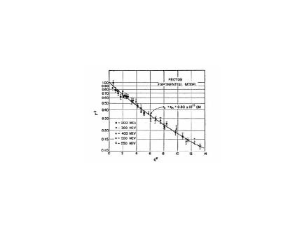
Figure 1: Fig. 27 in  [Hof56], with figure caption “The square of the FF plotted against ${\mathrm{q}}^{2}$.  ${\mathrm{q}}^{2}$ is given in units of $10^{26}cm^{-2}$. The solid line is calculated for the exponential model with rms radii=$0.80\times 10^{-13}$cm.”

Figure 2: Feynman diagram for the single-photon exchange, or Born term, for elastic $ep$ scattering.

In this early framework a phenomenological FF squared was obtained from absolute differential cross section measurements simply as:

$$[F({\mathrm{q}})]^{2}=\frac{\sigma({\mathrm{q}})}{\sigma_{Mott}({\mathrm{q}})},~{}~{}~{}\mbox{with }~{}~{}~{}\vec{q}=\vec{p}_{beam}-\vec{p}_{e}~{}\mbox{ and }~{}{\mathrm{q}}=|\vec{q}|,$$ (3)

where $\vec{q}$, $\vec{p}_{beam}$ and $\vec{p}_{e}$ are the center-of-mass (CM) momentum transfer, and incident and scattered electron momenta, respectively. The historically significant results of these measurements of the proton FF are in Fig. 2.

2.1.1 The Dirac and Pauli nucleon form factors

A direct connection between the reduced charge and magnetic moments discussed in [Ros50] and measurable observables was first proposed by Clementel and Villi [Cle56], who defined FFs on the basis of Rosenbluth’s discussion of effective charge and magnetic moments, following [Schi49], as $F_{1}(q)=\frac{e^{\prime}}{e}$ and $F_{2}(q)=\frac{\kappa^{\prime}e^{\prime}}{\kappa_{0}{e}}$, with $q=2\sqrt{E_{beam}E_{e}}\sin\frac{\theta_{e}}{2}$. These FFs were then introduced in experimental papers by Hofstadter and coworkers [Hof56, McA56, Hof58], who generalized the “effective” charge and magnetic moment concepts by associating the first with the deviation from a point charge Dirac particle (Dirac FF, $F_{1}$), and the second with the deviation from a point anomalous magnetic moment (Pauli FF, $F_{2}$).

In lowest order, elastic scattering of an electron by the proton is the result of the exchange of a single virtual photon of invariant mass squared ${q}^{2}=\omega^{2}-\vec{q}~{}^{2}=-4E_{beam}E_{e}\sin^{2}\frac{\theta_{e}}{2}$, (the last step neglects the electron mass), where $\omega=E_{beam}-E_{e}$, the energy loss of the electron, and $\vec{q}=\vec{p}_{beam}-\vec{p}_{e}$, the vector momentum change of the electron; $\theta_{e}$ is the Lab electron scattering angle. For scattering in the space like region, ${q}^{2}$ is negative.

The time-like region, where ${q}^{2}$ is positive, can be accessed for example in $e^{-}e^{+}\rightarrow{p}\bar{p}$ or ${p}\bar{p}\rightarrow e^{-}e^{+}$; it will not be discussed in this review.

Given the smallness of the fine structure constant $\alpha~{}\sim 1/137$, it has been common until recently, to neglect all higher order terms, except for the next order in $\alpha$ which is treated as a radiative correction, thus implicitly assuming that the single photon diagram, corresponding to the Born approximation, is determinant of the relation between cross section and FFs; we will revisit this point in section 3.5. In the single photon-exchange process illustrated in Fig. 2, and following the notation of [Rek02], the amplitude for elastic scattering can be written as the product of the four-component leptonic and hadronic currents, $\ell_{\nu}$ and ${\mathcal{J}}_{\mu}$ , respectively:

$$-i{\mathcal{M}}=\frac{-ig_{\mu\nu}}{{q}^{2}}\left[ie\bar{u}(p_{e})\gamma^{\nu}u(p_{beam})\right]\left[-ie\bar{N}(p^{\prime})\Gamma^{\mu}(p^{\prime},p)N(p)\right]=\frac{i}{{q}^{2}}\ell_{\mu}{\mathcal{J}}^{\mu},$$ (4)

where $\Gamma^{\mu}$ contains all information of the nucleon structure, $u$ and $N$ are the electron- and nucleon spinors, respectively, $g_{\mu\nu}$ is the metric tensor and $k$, $k^{\prime}$, $p$ and $p^{\prime}$ are the four-momenta of the incident and scattered electron and proton, respectively. To ensure relativistic invariance of the amplitude $\mathcal{M}$, $\Gamma^{\mu}$ can only contain $p$, $p^{\prime}$ and $\gamma^{\mu}$, besides scalars, masses and $Q^{2}$.

As was shown by Foldy [Fol52], the most general form for the hadronic current for a spin $\frac{1}{2}$-nucleon with internal structure, satisfying relativistic invariance and current conservation is:

$${\mathcal{J}}_{hadronic}^{\mu}=e\overline{N}(p^{\prime})\left[\gamma^{\mu}{{F_{1}(Q^{2})}}+\frac{i\sigma^{\mu\nu}q_{\nu}}{2M}{{F_{2}(Q^{2})}}\right]N(p),$$ (5)

where $Q^{2}=-{q}^{2}$, is the negative of the square of the invariant mass of the virtual photon in the one-photon-exchange approximation in $ep$ scattering, and $F_{1}$ and $F_{2}$ are the two only FFs allowed by relativistic invariance. Furthermore, the anomalous part of the magnetic moment for the proton is $\kappa_{p}=\mu_{p}-1$, and for the neutron $\kappa_{n}=\mu_{n}$, in nuclear magneton-units, $\mu_{N}=\frac{e\hbar}{2M}$, with values $\kappa_{p}=$1.7928 and $\kappa_{n}=-1.9130$, respectively; ${M}$ is the nucleon mass. It follows that in the static limit, $Q^{2}=0$, $F_{1p}(0)=1,F_{2p}(0)=\kappa_{p},F_{1n}(0)=0,F_{2n}(0)=\kappa_{n}$, for the proton and neutron, respectively.

In the one-photon-exchange approximation $F_{1}(Q^{2})$ and $F_{2}(Q^{2})$ are real functions which depend upon $Q^{2}$ only, and are therefore relativistically invariant. When higher order terms with two photons exchange are included, there are in general 6 invariant amplitudes, which can be written in terms of 3 complex ones [Gui03].

The Lab cross section is then:

$$\frac{d\sigma}{d\Omega_{e}}=\frac{\overline{|{\mathcal{M}}|}^{2}}{64\pi^{2}}\left(\frac{E_{2}}{E_{1}}\right)^{2}\frac{1}{M}~{}~{}~{}\mbox{ with }~{}~{}~{}\overline{|{\mathcal{M}}|}^{2}=\frac{1}{(Q^{2})^{2}}\overline{|\ell\cdot{\mathcal{J}}|}^{2},$$ (6)

Following the introduction above, we can now write the standard form for the Lab frame differential cross section for $ep$ or $en$ elastic scattering as:

$$\frac{d\sigma}{d\Omega_{e}}=\left(\frac{d\sigma}{d\Omega}\right)_{Mott}\frac{E_{e}}{E_{beam}}\left\{F_{1}^{2}(Q^{2})+\tau\left[F_{2}^{2}(Q^{2})+2\left(F_{1}(Q^{2})+F_{2}(Q^{2})\right)^{2}\tan^{2}\frac{\theta_{e}}{2}\right]\right\},$$ (7)

where $\tau=Q^{2}/4M^{2}$, and $\frac{E_{e}}{E_{beam}}=(1+\frac{2E_{beam}}{M}\sin^{2}\frac{\theta_{e}}{2})^{-1}=(1+\tau)^{-1}$ is the recoil factor. Eq. (7) is the most general form for the cross section, as required by Lorentz invariance, symmetry under space reflection and charge conservation. Experimentally, the first separate values for $F_{1}$ and $F_{2}$ were obtained by the intersecting ellipse method described by Hofstadter [Hof60]. The early data of Bumiller et al. [Bum60] showed that $F_{2}$ decreased with $q^{2}$ faster than $F_{1}$, even suggesting a diffractive behavior for the proton cross section. Typically these results show $F_{1}/F_{2}$-ratio values which are several times larger than modern values for the proton.

2.1.2 The electric and magnetic form factors

Another set of nucleon FFs, $F_{ch}$ and $F_{mag}$, was first introduced by Yennie, Levy and Ravenhall [Yen57]; Ernst, Sachs and Wali [Ern60] connected $F_{ch}$ and $F_{mag}$ to the charge and current distributions in the nucleon; the interpretation that $F_{ch}$ and $F_{mag}$ measure the interaction with static charge and magnetic fields was given by Walecka [Wal59]. The following FFs, $F_{ch}$ and $F_{mag}$, were defined in [Ern60]: $F_{ch}=F_{1}-\frac{Q^{2}}{2M}F_{2},~{}\mbox{and}~{}F_{m}=\frac{1}{2M}F_{1}+F_{2}$. A similar definition of FFs for charge and magnetization, $G_{E}$ and $G_{M}$, which is the one in use today, was first discussed extensively by Hand, Miller and Wilson [Han63] who noted that with $G_{E}=F_{1}-\tau F_{2}~{}\mbox{and}~{}G_{M}=F_{1}+F_{2}$, the scattering cross section in Eq. (7) can be written in a much simpler form, without interference term, leading to a simple separation method for $G_{Ep}^{2}$ and $G_{Mp}^{2}$:

$$\frac{d\sigma}{d\Omega}=\left(\frac{\alpha}{2E_{beam}\sin(\frac{\theta_{e}}{2})}\right)^{2}\frac{E_{e}}{E_{beam}}\left(\frac{\cot^{2}(\frac{\theta_{e}}{2})}{1+\tau}\left[G_{E}^{2}+\tau{G_{M}}^{2}\right]+2\tau{G_{M}}^{2}\right),$$ (8)

$G_{Ep}$, $G_{Mp}$, $G_{En}$ and $G_{Mn}$ are now customarily called the electric- and magnetic Sachs FFs, for the proton and neutron, respectively; at $Q^{2}=0$ they have the static values of the charge and magnetic moments, of the proton and neutron, respectively: $G_{Ep}(0)=1,G_{Mp}(0)=\mu_{p},G_{En}(0)=0~{}\mbox{and}~{}G_{Mn}(0)=\mu_{n}.$

2.1.3 Form factors in the Breit frame

The physical meaning of the electric and magnetic FFs, $G_{E}$ and $G_{M}$, is best understood when the hadronic current is written in the Breit frame. In that frame the scattered electron transfers momentum $\vec{q}_{B}$ but no energy ($\omega_{B}=0$). Therefore, the proton likewise undergoes only a change of momentum, not of energy, from $-\vec{q}_{B}/2$ to $+\vec{q}_{B}/2$; thus $Q^{2}=\vec{q_{B}}^{2}$. The four components of the hadronic current in the Breit frame are:

$$J^{0} = e2M{\chi^{\prime\dagger}}\chi(F_{1}-{\tau}{F_{2}})=e2M{\chi^{\prime\dagger}}{\chi}G_{E},$$ (9)

$$\vec{J} = ie\chi^{\prime\dagger}(\vec{\sigma}\times\vec{q}_{B})\chi(F_{1}+{F_{2}})=ie\chi^{\prime\dagger}(\vec{\sigma}\times\vec{q}_{B})\chi{G_{M}}.$$ (10)

Only in the Breit frame can the electric and magnetic FFs $G_{E}$ and $G_{M}$ be associated with charge and magnetic current density distributions through a Fourier transformation. However the Breit frame is a mathematical concept without physical reality: there is a Breit frame for every $Q^{2}$ value; and above a few GeV², the Breit frame moves in the Lab with relativistic velocities, resulting in a non-trivial relation between Breit frame quantities and Lab frame quantities: the transformation affects both the kinematics and the structure. A model dependent procedure to transform these distributions from the Breit– to the Lab frame has been recently developed by Kelly [Kel02], with interesting results to be discussed later in section 4.3.

2.2 Rosenbluth form factor separation method

The Rosenbluth method has been the only technique available to obtain separated values for $G_{E}^{2}$ and $G_{M}^{2}$ for proton and neutron until the 1990s. The method requires measuring the cross section for $eN$ scattering at a number of electron scattering angles, for a given value of $Q^{2}$; this is obtained by varying both the beam energy and the electron scattering angle over as large a range as experimentally feasible.

The cross section for $ep$ scattering in Eq. (7), when written in terms of the electric- and magnetic FFs, $G_{E}$ and $G_{M}$, takes the following form:

$$\frac{d\sigma}{d\Omega}=\left(\frac{d\sigma}{d\Omega}\right)_{Mott}\times\left(G_{E}^{2}+\tau\left[1+2(1+\tau)\tan^{2}\frac{\theta_{e}}{2}\right]G_{M}^{2}\right)/(1+\tau),$$ (11)

and in the notation preferred today, this cross section can be re-written as:

$$\frac{d\sigma}{d\Omega}=\left(\frac{d\sigma}{d\Omega}\right)_{Mott}\times\left[G_{E}^{2}+\frac{\tau}{\epsilon}G_{M}^{2}\right]/(1+\tau),$$ (12)

where $\epsilon=[{1+2(1+\tau)\tan^{2}\frac{\theta_{e}}{2}}]^{-1}$ is the virtual photon polarization.

In early versions of the Rosenbluth separation method for the proton, a correspondingly defined reduced cross section was plotted either as a function of $\cot^{2}\frac{\theta_{e}}{2}$ [Han63, Wil64] or $\cos\theta_{e}$ [Ber71]. For example in [Han63], the function $R(Q^{2},\theta_{e})=\left[G_{E{p}}^{2}+\tau{G}_{M{p}}^{2}\right]\cot^{2}\frac{\theta_{e}}{2}+\tau(1+\tau)G_{M{p}}^{2}$ was defined. In 1973 Bartel et al. chose a form linear in ${\cos^{2}\frac{\theta_{e}}{2}}$, namely $\cos^{2}\frac{\theta_{e}}{2}\times\left(\frac{d\sigma}{d\Omega}\right)/\left(\frac{d\sigma}{d\Omega}\right)_{Mott}$ [Bar73]. Neither of these linearization procedures fully disentangles $G_{E{p}}^{2}$ and $G_{M{p}}^{2}$.

The modern version of the Rosenbluth separation technique takes advantage of the linear dependence in $\epsilon$ of the FFs in the reduced cross section based on Eq. (12) and is defined as follows:

$$\left(\frac{d\sigma}{d\Omega}\right)_{reduced}=\frac{\epsilon(1+\tau)}{\tau}\left(\frac{d\sigma}{d\Omega}\right)_{exp}/\left(\frac{d\sigma}{d\Omega}\right)_{Mott}=G_{M}^{2}+\frac{\epsilon}{\tau}G_{E}^{2},$$ (13)

where $(d\sigma/d\Omega)_{exp}$ is a measured cross section. A fit to several measured reduced cross section values at the same $Q^{2}$, but for a range of $\epsilon$-value, gives independently $\frac{1}{\tau}G_{E{p}}^{2}$ as the slope and $G_{M{p}}^{2}$ as the intercept, as shown in Fig. 4; the data displayed in this figure are taken from [And94].

Figure 3: Demonstration of the Rosenbluth separation method based on the data from  [And94]. The $Q^{2}$ values shown are 2.5 (open triangle), 5.0 (circle) and 7.0 (filled triangles) GeV².

Figure 4: Early Rosenbluth separation data for $G_{Ep}$, up to 1973 [Ber71, Pri71, Bar73, Han73], but not including the 1970 SLAC experiment of Litt et al. [Lit70].

2.2.1 Proton form factor measurements

Figure 4 shows Rosenbluth separation results performed in the 1970’s as the ratio $G_{E{p}}/G_{D}$, where $G_{D}$ is the dipole FF given below by Eq. 14; it is noteworthy that these results strongly suggest a decrease of $G_{Ep}$ with increasing $Q^{2}$, a fact noted in all four references [Ber71, Pri71, Bar73, Han73]. As will be seen in section 3.4, the slope of this decrease is about half the one found in recent recoil polarization experiments. Left out of this figure are the data of Litt et al. [Lit70], the first of a series of SLAC experiments which were going to lead to the concept of “scaling” based on Rosenbluth separation results, namely the empirical relation $\mu_{p}G_{E{p}}/G_{M{p}}\sim 1$. Predictions of the proton FF $G_{E{p}}$ made in the same period and shown in Fig. 4 are from Refs. [Iac73, Hoh76, Gar85], all three are based on a dispersion relation description of the FFs, and related to the vector meson dominance model (VMD).

Figure 5: Data base for $G_{E{p}}$ obtained by the Rosenbluth method; the references are [Han63, Lit70, Pri71, Ber71, Bar73, Han73, Bor75, Sim80, And94, Wal94, Chr04, Qat05].

Figure 6: Data base for $G_{M{p}}$ obtained by the Rosenbluth method; the references are [Han63, Jan66, Cow68, Lit70, Pri71, Ber71, Han73, Bar73, Bor75, Sil93, And94, Wal94, Chr04, Qat05].

Figure 7: The $G_{Mp}$ data follow the pQCD scaling law, $G_{Mp}\propto\frac{1}{Q^{4}}$, as was first demonstrated in [Arn86]; data as in Fig. 6.

Figure 8: Fig. 4 from Ref. [Gao03]. The 1990 Platchkov data [Pla90] for $G_{En}$, with fits to several NN potentials determining the deuteron wave function.

A compilation of all $G_{Ep}$ and $G_{Mp}$ data obtained by the the Rosenbluth separation technique is shown in Figs. 6 and 6; in these two figures both $G_{Ep}$ and $G_{Mp}$ have been divided by the dipole FF $G_{D}$ given by:

$$G_{D}=\frac{1}{(1+Q^{2}/0.71{\mathrm{G}eV^{2}})^{2}}~{}~{}\mbox{with}~{}~{}G_{Ep}=G_{D},~{}G_{Mp}=\mu_{p}G_{D},~{}~{}\mbox{and}~{}~{}G_{Mn}=\mu_{n}G_{D}.$$ (14)

It is apparent from Fig. 6 that the cross section data have lost track of $G_{Ep}$ above $Q^{2}\sim 1$ GeV². It is difficult to obtain $G_{E}^{2}$ for large $Q^{2}$ values by Rosenbluth separation from $ep$ cross section data for several reasons; first, the factor $\frac{1}{\tau}$ multiplying $G_{E}^{2}$ in Eq. (13) automatically reduces the contribution of this term to the cross section as $Q^{2}$ increases; and second, even at small $Q^{2}$, $G_{M}^{2}\sim\mu_{p}^{2}G_{E}^{2}$, hence the contribution of $G_{E}^{2}$ to the cross section is reduced by a factor 7.80.

In sharp contrast with the situation for $G_{Ep}$, the $G_{Mp}/\mu_{p}G_{D}$ ratios shown in Fig. 6 display excellent internal consistency, up to $Q^{2}=30$ GeV², for the $G_{Mp}$-values obtained from cross section data; note that the large $Q^{2}$- data in [Arn86] were obtained without Rosenbluth separation, with the assumption that $G_{Ep}=G_{Mp}/\mu_{p}$; the ratio $G_{Mp}/\mu_{p}G_{D}$ becomes distinctly smaller than 1 above $\sim$ 5 GeV².

It was first observed by Arnold et al. [Arn86] that the proton magnetic FF, $G_{Mp}$ follows the pQCD prediction of Brodsky and Farrar [Bro75], as illustrated in Fig. 8; the pQCD prediction is based on quark counting rules. Indeed $Q^{4}G_{Mp}$ becomes nearly constant starting at $Q^{2}=8$ GeV². However, the $1/Q^{4}$-behavior of the proton magnetic FF was first mentioned by Coward et al. [Cow68] based on their data extending to 20 GeV²; these authors discussed the 1/$Q^{4}$ behavior in light of the vector meson exchange model prevailing at the time [SchW67].

2.2.2 Neutron electric form factor measurements

The “neutrality” of the neutron requires the electric FF to be zero at $Q^{2}=0$, and small at non-zero $Q^{2}$; historically, the fact that the electric FF is non-zero has been explained in terms of a negatively charged pion cloud in the neutron, which surrounds a small positive charge [Fer47].

Early attempts to determine the neutron FF were based on measurements of the elastic $ed$ cross section. The scattering by an electron from the spin 1 deuteron requires 3 FFs in the hadronic current operator, for the charge, quadrupole and magnetic distributions, $G_{C}$, $G_{Q}$ and $G_{M}$, respectively. In the original impulse approximation (IA) form of the cross section developed by Gourdin [Gou64], the elastic $ed$ cross section is:

$$\frac{d\sigma}{d\Omega}=\frac{d\sigma}{d\Omega}_{Mott}\left(A(Q^{2})+B(Q^{2})\tan^{2}(\frac{\theta_{e}}{2})\right),$$ (15)

where $A(Q^{2})=G_{C}^{2}(Q^{2})+\frac{8}{9}\eta^{2}G_{Q}^{2}(Q^{2})+\frac{2}{3}\eta(1+\eta)G_{M}^{2}$ and $B(Q^{2})=\frac{3}{4}\eta(1+\eta)^{2}G_{M}^{2}(Q^{2})$, with $\eta=Q^{2}/4M_{D}^{2}$.
The charge, quadrupole and magnetic FFs can be written in terms of the isoscalar electric and magnetic FFs   as follows:

$G_{C}=G_{E}^{S}C_{E},~{}~{}\mbox{ }~{}~{}G_{Q}=G_{E}^{S}C_{Q}~{}~{}\mbox{ and }~{}~{}G_{M}=\frac{M_{D}}{M_{p}}(G_{M}^{S}C_{S}+\frac{1}{2}G_{E}^{S}C_{L})$,

where the coefficients $C_{E}$, $C_{Q}$, $C_{L}$ and $C_{S}$ are Fourier transforms of specific combinations of the S- and D-state deuteron wave functions, $u(r)$ and $w(r)$ [Gou64].

The 1971 DESY experiment of Galster et al. [Gal71] measured elastic $ed$ cross sections up to 0.6 GeV² with good accuracy and provided a data base for the extraction of $G_{En}$; it had been preceded by a series of experiments started at the Stanford MARK III accelerator, including McIntyre and Dhar [McI57], Friedman, Kendall and Gram [Fri60], Drickey and Hand [Dri62], Benaksas, Drickey and Frèrejacque [Ben64], and Grossetête, Drickey and Lehmann [Gro66a]. On the basis of these data, and using Hamada-Johnston [Ham62] and Feshbach-Lomon [Fes67] deuteron wave functions, the following fitting function was proposed in [Gal71]:

$$G_{En}(Q^{2})=-\frac{\mu_{n}\tau}{1+5.6\tau}G_{Ep}(Q^{2}).$$ (16)

The often quoted Galster fit uses Eq. (16) with $G_{Ep}$ replaced by the dipole FF $G_{D}$ (see Eq. (14)).

The next and last experiment to measure the elastic $ed$ cross section to determine $G_{En}$ is that of Platchkov et al. [Pla90]. These data extend to $Q^{2}$ of 0.7 GeV², with significantly smaller statistical uncertainties than all previous experiments. The data from Platchkov et al. [Pla90] are shown in Fig. 8. The FF $A(Q^{2})$ is very sensitive to the deuteron wave function, and therefore to the $NN$ interaction. Furthermore, the shape of $A(Q^{2})$ cannot be explained by the IA alone. Corrections for meson exchange currents (MEC) and a small contribution from relativistic effects were found to significantly improve the agreement between calculations and the shape of $A(Q^{2})$ observed. The authors included the constraint from the slope of the neutron electric FF as determined in $ne$ scattering, which at the time was $dG_{En}/dQ^{2}$=0.0199 fm² [Koe76]; they proposed a modified form of the Galster fit using several $NN$ potentials, and including MEC as well as relativistic corrections, of the form $G_{En}(Q^{2})=-a\frac{\mu_{n}\tau}{1+b\tau}G_{Ep}(Q^{2})$, corresponding to a slope at $Q^{2}=0$: $dG_{En}/dQ^{2}=-a\mu_{n}/4M^{2}$. For the Paris $NN$ potential for example, $a$=1.25 and $b$=18.3; this fit will be compared with the double-polarization data shown later in this review, in Fig. 21. Starting in 1994, all $G_{En}$ measurements have used either polarization transfer or beam-target asymmetry to take advantage of the interference nature of these observables: terms proportional to $G_{En}G_{Mn}$ are measured, instead of the $G_{En}^{2}$ contribution to the cross section; these experiments will be reviewed in section 3.3.

2.2.3 Neutron magnetic form factor measurements

In an early experiment Hughes et al. [Hug65] performed a Rosenbluth separation of quasi elastic $d(e,e^{\prime})$ cross sections in the range $Q^{2}=0.04$ to 1.17 GeV²; they observed non-zero values of $G_{En}$ only below 0.2 GeV² but measured $G_{Mn}$ up to 1.17 GeV²; the technique consisted in comparing quasi-elastic $ed$- with elastic $ep$ cross sections. The several experiments following Hughes’ can be subdivided into 3 groups: cross section measurements in quasi-elastic $ed$ scattering (single arm) [Han73, Bar73], which requires large final state interaction (FSI) corrections at small $Q^{2}$; elastic $ed$ cross section measurements [Ben64, Gro66b]; and cross section measurements in $d(e,e^{\prime}p)n$ [Bud68, Dun66], or ratio of cross sections $d(e,e^{\prime}n)p/d(e,e^{\prime}p)n$ [Ste66], which is less sensitive to the deuteron wave function, and MEC.

Figure 9: Early Rosenbluth separation data for $G_{Mn}$, up to 1973 [Ben64, Hug65, Gro66b, Ste66, Dun66, Bud68, Han73, Bar73].

Figure 10: Recent $G_{Mn}$ data divided by $\mu_{n}G_{D}$, from cross section data only, starting in 1992 [Roc92, Lun93, Mar93, Ank94, Bru95, Ank98, Kub02, Bro05].

All results published prior to 1973 are displayed in Fig. 10, to be compared with the proton data from the same period in Fig. 4. All more recent cross section results are in Fig. 10, allowing for a comparison of the progress made in this period for the neutron. In Fig. 10 all $G_{Mn}$ data obtained from cross section measurements are displayed, including the SLAC experiments [Roc92, Lun93], which measured inclusive quasi-elastic $ed$ cross sections. The more recent ELSA [Bru95] and MAMI [Ank94, Ank98, Kub02] experiments are simultaneous measurements of the cross section for quasi elastic scattering on the neutron and proton in the deuteron, $d(e,e^{\prime}n)p$ and $d(e,e^{\prime}p)n$; the systematics is then dominated by the uncertainty in the neutron detector efficiency; much attention was given to that calibration in these experiments. In the ELSA experiment [Bru95] protons and neutrons were detected in the same scintillator, and the neutron efficiency was determined in situ with the neutrons from ${}^{1}H(\gamma,\pi)$. It has been argued in [Jou97] that 3-body electro-production contributes significantly and does not necessarily lead to a neutron at the 2-body kinematic angle; these data points are shown as $\diamondsuit$ in Fig.10; a refutation of these arguments is in [Bru97]. In the Mainz experiments the dedicated neutron detector was calibrated in a neutron beam at SIN. The new data from Hall B at JLab, [Bro05], are shown as filled triangles in Fig. 10; for these data from Hall B, in addition to the measurements of cross section ratio with the ${}^{2}H$ target, an in-line ${}^{1}H$ target was used for an in-situ determination of the neutron counter efficiency via $\pi^{+}$ electro-production.

2.2.4 Rosenbluth results and dipole form factor

In figures 13, 13 and 13 the Rosenbluth separation results $G_{Ep}$, $G_{Mp}$ and $G_{Mn}$ are shown in double logarithmic plots for $Q^{2}<2$ GeV², to emphasize the good agreement of these data with the dipole formula of Eq. 14.

Noticeable is the lack of $G_{Mp}$ and $G_{Mn}$ data below $Q^{2}$ of 0.02 GeV², a consequence of the dominance of the electric FF at small $Q^{2}$ for the proton, as seen in Eq. (12).

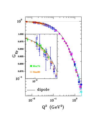
Figure 11: Illustration of the quality of the dipole fit for $G_{E{p}}$; data from Refs. [Han63, Lit70, Pri71, Ber71, Han73, Bar73, Mur74, Bor75, Sim80, Wal94, And94] in $Q^{2}$ range 0.005-2.0 GeV².

Figure 12: Illustration of the quality of the dipole fit for $G_{Mp}$; the data of Refs. [Han63, Jan66, Lit70, Pri71, Ber71, Han73, Bar73, Bor75, Wal94] in the range 0.005-2.0 GeV² are included here.

Figure 13: Illustration of the quality of the dipole fit for $G_{M{n}}$; the data included are the same as in Fig. 10, Refs. [Roc92, Lun93, Mar93, Ank94, Bru95, Ank98, Kub02, Bro05] in the $Q^{2}$-range 0.005-2.0 GeV².

Although Hofstadter was the first to note that the proton FF data could be fitted by an “exponential model”, which corresponds to the “dipole model” for FFs in momentum space, it appears that the usage of dividing data by $G_{D}$ was introduced first by Goitein et al. [Goi67].

The possible origin of the dipole FF has been discussed in a number of early papers. Within the framework of dispersion theory the isovector and isoscalar parts of a FF is written as, $G_{E,M}^{V,S}=\Sigma_{i}\frac{\alpha_{i}^{V,S}}{1+Q^{2}/(M_{i}^{V,S})^{2}}$, where $G_{E,M}^{V},\mbox{ }G_{E,M}^{S}$ are defined in footnote 2, and $M_{i}^{V,S}$ and $\alpha_{i}^{V,S}$ are the masses and residua of the isovector-, isoscalar vector mesons, respectively. A dipole term occurs when the contribution of two vector mesons with opposite residua but similar masses are combined.

3 Nucleon form factors from double polarization observables

It was pointed out in 1968 by Akhiezer and Rekalo [Akh68] that “for large momentum transfers the isolation of the charge FF of the proton is difficult” using the elastic $ep$ reaction with an unpolarized electron beam, for several reasons: one being $G_{Mp}^{2}/G_{Ep}^{2}\geq\mu_{p}^{2}$ at any $Q^{2}$ value and the other is that at large $Q^{2}$ the contribution from the $\tau G_{Mp}^{2}$ term in $G_{Ep}^{2}+(\tau/\epsilon)G_{Mp}^{2}$ increases (see Eq.( 12)) and makes the separation of the charge form factor practically impossible. In the same paper the authors also pointed out that the best way to obtain the proton charge FF is with polarization experiments, especially by measuring the polarization of the recoil proton. Further in a review paper in 1974 Akhiezer and Rekalo [Akh74] discussed specifically the interest of measuring an interference term of the form $G_{E}G_{M}$ by measuring the transverse component of the recoiling proton polarization in the $\vec{e}p\rightarrow e\vec{p}$ reaction at large $Q^{2}$, to obtain $G_{E}$ in the presence of a dominating $G_{M}$. In 1969, in a review paper Dombey [Dom69] also discussed the virtues of measuring polarization observables in elastic and inelastic lepton scattering; however his emphasis was to do these measurements with a polarized lepton on a polarized target. Furthermore in 1982 Arnold, Carlson and Gross [Arn81]emphasized that the best way to measure the electric FF of the neutron would be to use the ${}^{2}H(\vec{e},e^{\prime}\vec{n})p$ reaction. Both a polarized target, and a focal plane polarimeter (to measure recoil polarization), have been used to obtain nucleon FFs. We discuss below both methods to measure the elastic nucleon FFs, highlighting advantages and disadvantages of using polarized target and focal plane polarimeter.

3.1 Polarization transfer

Figure 15 shows the kinematical variables for the polarization transfer from a longitudinally polarized electron to a struck proton in the one-photon exchange approximation.

Figure 14: Kinematical variables for polarization transfer from a longitudinally polarized electron to a proton with exchange of a virtual photon.

Figure 15: Polarized electron scattering from a polarized target.

The electron vertex in Fig. 15 can be described by basic Quantum Electrodynamics (QED) rules that involves the electron current, $\ell_{\mu}$, and the proton vertex can be described by QCD and hadron electrodynamics involving the hadronic current $J^{\mu}=\chi^{\prime\dagger}F_{\mu}\chi$.

For elastic $ep$ scattering with longitudinally polarized electrons, the hadronic tensor, $W_{\mu\nu}$= $J_{\mu}J_{\nu}^{*}$, has four possible terms depending upon the polarization of the target and of the recoil proton:

$$W_{\mu\nu}~{}=~{}W_{\mu\nu}^{(o)}+W_{\mu\nu}({\bf P_{1}})+W_{\mu\nu}({\bf P_{2}})+W_{\mu\nu}({\bf P_{1},P_{2}}),$$ (17)

where the first term in the equation corresponds to unpolarized protons, the second and the third term correspond to the vector polarization of the initial and the final proton, respectively, and the last term describes the reaction when both, the initial and the final protons are polarized.

Considering the case where only the polarization of the final proton is measured, $W_{\mu\nu}({\bf P})$ is:

$$W_{\mu\nu}({\bf P})~{}=~{}\frac{1}{2}TrF_{\mu}F_{\nu}^{\dagger}\vec{\sigma}\cdot{\bf P}.$$ (18)

For the scattering of longitudinally polarized electrons off an unpolarized target, in the one-photon-exchange approximation, there are only two non-zero polarization components, transverse, $P_{x}$, and longitudinal, $P_{z}$; and these components are obtained by calculating the tensors $W_{\mu\nu}(P_{x})=\frac{1}{2}TrF_{\mu}F_{\nu}^{\dagger}\sigma_{x}\sim 2mG_{E}G_{M}$ and $W_{\mu\nu}(P_{z})=\frac{1}{2}TrF_{\mu}F_{\nu}^{\dagger}\sigma_{z}\sim G_{M}^{2}$.

The transformation from Breit to laboratory frame gives following expressions for the polarization components $P_{x}$ and $P_{z}$ in terms of the electric $G_{E}$, and magnetic, $G_{M}$ FF [Akh74, Arn81];

$$I_{0}P_{x} = -2\sqrt{\tau(1+\tau)}G_{E}G_{M}\tan\frac{\theta_{e}}{2}$$ (19)

$$I_{0}P_{z} = \frac{1}{M}(E_{beam}+E_{e})\sqrt{\tau(1+\tau)}G_{M}^{2}\tan^{2}\frac{\theta_{e}}{2},$$ (20)

where $E_{beam}$ and $E_{e}$ are the energy of the incident and scattered electrons, respectively, $\theta_{e}$ is the scattered electron angle in the laboratory frame, and $I_{0}$ is:

$$I_{0}=G_{E}^{2}(Q^{2})+\frac{\tau}{\epsilon}G_{M}^{2}(Q^{2}).$$ (21)

Eqs. (19) and  (20) show that the transverse and longitudinal polarization components are proportional to $G_{E}G_{M}$ and $G_{M}^{2}$, respectively. The ratio $G_{E}/G_{M}$ then can be obtained directly from the ratio of the two polarization components $P_{x}$ and $P_{z}$ as follows:

$$\frac{G_{E}}{G_{M}}=-\frac{P_{x}}{P_{z}}\frac{(E_{beam}+E_{e})}{2M}\tan(\frac{\theta_{e}}{2}).$$ (22)

Equation (22) makes clear that this method offers several experimental advantages over the Rosenbluth separation: (1) for a given $Q^{2}$, only a single measurement is necessary, if the polarimeter can measure both components at the same time. This greatly reduces the systematic errors associated with angle and beam energy change, and (2) the knowledge of the beam polarization and of the analyzing power of the polarimeter is not needed to extract the ratio, $G_{E}/G_{M}$.

3.2 Asymmetry with polarized targets

It was pointed out by Dombey [Dom69] that the nucleon FFs can be extracted from the scattering of longitudinally polarized electrons off a polarized nucleon target. In the one-photon-exchange approximation, following the approach of Donnelly and Raskin [Don86, Ras86], the elastic $eN$ ($N=p$ or $n$) cross section can be written as a sum of an unpolarized part and a polarized part; the latter is non-zero only if the electron beam is longitudinally polarized:

$$\sigma^{pol}=\Sigma+h\Delta,\\$$ (23)

where $h$ is the electron beam helicity, $\Sigma$ is the elastic un-polarized cross section given by Eq. (12), and $\Delta$ is the polarized part of the cross section with two terms related to the directions of the target polarization. The expression for $\Delta$ can be written as [Don86, Ras86]:

$$\Delta=-2\sigma_{Mott}\tan(\theta_{e}/2)\sqrt{\frac{\tau}{1+\tau}}{\Biggl{\{}\sqrt{\tau[1+(1+\tau)\tan^{2}(\theta_{e}/2)]}\cos\theta^{\ast}G_{M}^{2}+\sin\theta^{\ast}\cos\phi^{\ast}G_{E}G_{M}\Biggr{\}}}$$ (24)

where $\theta^{\ast}$ and $\phi^{\ast}$ are the polar and azimuthal laboratory angles of the target polarization vector with $\vec{q}$ in the $\vec{u}_{z}$ direction and $\vec{u}_{y}$ normal to the electron scattering plane, as shown in Figure 15.

The physical asymmetry $A$ is then defined as

$$A=\frac{\sigma_{+}-\sigma_{-}}{\sigma_{+}+\sigma_{-}}=\frac{\Delta}{\Sigma},$$ (25)

where $\sigma_{+}$ and $\sigma_{-}$ are the cross sections for the two beam helicities.

For a polarized target, the measured asymmetry, $A_{meas}$, is related to the physical asymmetry, $A$, by

$$A_{meas}=P_{beam}P_{target}A,$$ (26)

where $P_{beam}$ and $P_{target}$ are electron beam- and target polarization, respectively, and,

$$A = -\frac{2\sqrt{\tau(1+\tau)}\tan(\theta_{e}/2)}{G_{E}^{2}+\frac{\tau}{\epsilon}G_{M}^{2}}\Big{[}\sin\theta^{\ast}\cos\phi^{\ast}G_{E}G_{M}+\sqrt{\tau[1+(1+\tau)\tan^{2}(\theta_{e}/2)]}\cos\theta^{\ast}G_{M}^{2}\Big{]}.$$ (27)

It is evident from Eq. (27) that to extract $G_{E}$, the target polarization in the laboratory frame must be perpendicular with respect to the momentum transfer vector ${\vec{q}}$ and within the reaction plane, with $\theta^{\ast}=\pi/2$ and $\phi^{\ast}=0^{o}$ or $180^{o}$. For these conditions, the asymmetry $A$ in Eq. (27) simplifies to:

$$A_{perp}=\frac{-2\sqrt{\tau(1+\tau)}\tan(\theta_{e}/2)\frac{G_{E}}{G_{M}}}{(\frac{G_{E}}{G_{M}})^{2}+\frac{\tau}{\epsilon}}.$$ (28)

As $(G_{E}/G_{M})^{2}$ is quite small, $A_{perp}$ is approximately proportional to $G_{E}/G_{M}$. In practice, the second term in Eq. (27) is not strictly zero due to the finite acceptance of the detectors, but these effects are small and depend on kinematics only in first order and can be corrected for, so the ratio $G_{E}/G_{M}$ is not affected directly.

The discussion described above is only applicable to a free nucleon; corrections are required if nuclear targets, like ²H or ³He, are used instead in quasi-elastic scattering to obtain the FFs.

3.3 Double polarization experiments

The polarization method, using polarized targets and focal plane polarimeter with longitudinally polarized electron beam, has been used to measure both the proton and the neutron e.m. FFs. Below we first describe the polarization experiments that measured the proton FFs and next those that measured the neutron FFs.

3.3.1 Proton form factor measurements with polarization experiments

The first experiment to measure the proton polarization observable in $ep$ elastic scattering was done at the Stanford Linear Accelerator Center (SLAC) by Alguard et al. [Alg76]. They measured the anti-parallel-parallel asymmetry in the differential cross sections by scattering longitudinally polarized electrons on polarized protons. From their result they concluded that the signs of $G_{Ep}$ and $G_{Mp}$ are the same; they also noted that the usefulness of using polarized beam on polarized target is severely limited by low counting rates.

Next, the recoil polarization method to measure the proton e.m. FF was used at MIT-Bates laboratory [Mil98, Bar99]. In this experiment the proton FF ratio $G_{Ep}/G_{Mp}$ was obtained for a free proton and a bound proton in a deuterium target at two $Q^{2}$ values, 0.38 and 0.5 GeV² using polarization transfer from longitudinally polarized electron to the proton in the target, and measuring the polarization of the recoiling proton with a focal plane polarimeter (FPP). The conclusion from these measurements was that the polarization transfer technique showed great promise for future measurements of $G_{Ep}$ and $G_{En}$ at higher $Q^{2}$ values.

The ratio $G_{Ep}/G_{Mp}$ in elastic ${}^{1}H(\vec{e},e^{\prime}\vec{p})$ was also measured at the MAMI in a dedicated experiment [Pos01], and as a calibration measurement [Die01] at a $Q^{2}$ of $\approx$0.4 Gev². The ratio values found were in agreement with other polarization measurements as well as Rosenbluth measurements. Most recently the BLAST group at MIT-Bates [Cra06] measured the ratio $G_{Ep}/G_{Mp}$ at $Q^{2}$ values of 0.2 to 0.6 GeV² with high precision.

Starting in late 1990’s, the proton FF ratios $G_{Ep}/G_{Mp}$ were measured in two successive dedicated experiments in Hall A at JLab for $Q^{2}$ from 0.5 to 5.6 GeV² [Jon00, Gay02, Pun05]. Other measurements were also conducted in Hall A [Gay01, Str03, Hu06] at lower $Q^{2}$ values, as calibration measurements for other polarization experiments, and one measurement in Hall C [MacL06].

In the first JLab experiment the ratio, $G_{Ep}/G_{Mp}$, was measured up to $Q^{2}$ of 3.5 GeV² [Jon00, Pun05]. Protons and electrons were detected in coincidence in the two high-resolution spectrometers (HRS) of Hall A [Alc04]. The polarization of the recoiling proton was obtained from the asymmetry of the azimuthal distribution after the proton re-scattered in a graphite analyzer.

The ratio, $G_{Ep}/G_{Mp}$, was measured at $Q^{2}$ = 4.0, 4.8 and 5.6 GeV² with an overlap point at $Q^{2}$ = 3.5 GeV²  [Gay02], in the second JLab experiment. To extend the measurement to higher $Q^{2}$, two changes were made from the first experiment. First, to increase the figure-of-merit (FOM) of the FPP, a CH₂ analyzer was used instead of graphite; hydrogen has much higher analyzing power [Spi83, Mil77] than carbon [Che95]. Second, the thickness of the analyzer was increased from 50 cm of graphite to 100 cm of CH₂ to increase the fraction of events with a second scattering in the analyzer. Third, the electrons were detected in a lead-glass calorimeter with a large frontal area, to achieve complete solid angle matching with the HRS detecting the proton. At the largest $Q^{2}$ of 5.6 GeV² the solid angle of the calorimeter was 6 times that of the HRS.

Proton polarimeters are based on nuclear scattering from an analyzer material like graphite or CH₂; the proton-nucleus spin-orbit interaction and proton-proton spin dependent interaction results in an azimuthal asymmetry in the scattering distribution which can be analyzed to obtain the proton polarization. The detection probability for a proton scattered by the analyzer with polar angle $\vartheta$ and azimuthal angle $\varphi$ is given by:

$$f^{\pm}(\vartheta,\varphi)=\frac{\epsilon(\vartheta,\varphi)}{2\pi}\left(1\pm A_{y}(P_{x}^{fpp}\sin{\varphi}-P_{y}^{fpp}\cos{\varphi})\right),$$ (29)

where $\pm$ refers to the sign of the beam helicity, $P_{x}^{fpp}$ and $P_{y}^{fpp}$ are transverse and normal polarization components in the reaction plane at the analyzer, respectively, and $\epsilon(\vartheta,\varphi)$ is an instrumental asymmetry that describes a non-uniform detector response. Physical asymmetries are obtained from the difference distribution of $f^{\pm}$,

$$D_{i} = (f^{+}_{i}-f^{-}_{i})/2~{}=~{}\frac{1}{2\pi}\left(A_{y}P_{x}^{fpp}\sin{\varphi_{i}}-A_{y}P_{y}^{fpp}\cos{\varphi_{i}}\right),$$ (30)

and the sum distribution of $f^{\pm}$ separates the instrumental asymmetries $\epsilon_{i}$,

$$E_{i} = (f^{+}_{i}+f^{-}_{i})/2~{}=~{}\frac{\epsilon_{i}}{2\pi}.$$ (31)

The values of the two asymmetries at the FPP, $A_{y}P_{x}^{fpp}$ and $A_{y}P_{y}^{fpp}$, can be obtained by Fourier analysis of the difference distribution $D_{i}$; however to calculate the ratio $G_{Ep}/G_{Mp}$, the proton polarization components $P_{x}$ and $P_{z}$ are needed at the target.

As the proton travels from the target to the focal plane through the magnetic elements of the HRS, its spin precesses, and therefore the polarization components at the FPP and at the target are different. The hadron HRS in Hall A consists of three quadrupoles and one dipole with shaped entrance and exit edges, as well as a radial field gradient. The polarization vectors at the polarimeter, $\vec{P}^{fpp}$, are related to those at the target, $h\vec{P}$, through a 3-dimensional spin rotation matrix, $(\bf S)$, as follows:

$\left(\begin{array}[]{c}P_{y}^{fpp}\\ P_{x}^{fpp}\\ P_{z}^{fpp}\end{array}\right)=\left(\begin{array}[]{ccc}S_{yy}&S_{yx}&S_{yz}\\ S_{xy}&S_{xx}&S_{xz}\\ S_{zy}&S_{zx}&S_{zz}\end{array}\right)\left(\begin{array}[]{c}P_{y}\\ P_{x}\\ P_{z}\end{array}\right)$.

The spin transport matrix elements $S_{ij}$ can be calculated using a model of the HRS with quadrupoles, fringe fields, and radial field gradient in the dipole, for each tuning of the spectrometer setting, and event by event with the differential-algebra-based transport code COSY [Ber95]. The spin transport method to obtain the two asymmetries at the target, $hA_{y}P_{x}$ and $hA_{y}P_{z}$, was developed by Pentchev and described in detail in [Pen03], and discussed in [Pun05]. The ratio $G_{Ep}/G_{Mp}$ was calculated from the two asymmetries at the target from Eq. (22). The fact that both beam polarization, and polarimeter analyzing power cancel out of this equation contributes to the reduction of the systematic uncertainties, however their values do influence the statistical errors.

The most recent acquisition of the FF ratio $G_{Ep}/G_{Mp}$ has been made at a $Q^{2}$ of 1.51 GeV² by measuring the beam-target asymmetry in an experiment in Hall C at JLab in elastic $ep$ scattering [Jon06]. This is the highest $Q^{2}$ at which the $G_{Ep}/G_{Mp}$ ratio has been obtained from a beam-target asymmetry measurement.

The results from the two JLab experiments [Gay02, Pun05], and other polarization measurements [Mil98, Gay01, Pos01, Die01, Str03, Hu06, MacL06, Jon06], are plotted in Fig. 17 as the ratio $\mu_{p}G_{Ep}/G_{Mp}$ versus $Q^{2}$. All data show only the statistical uncertainty; the systematic uncertainty for the data of [Gay02, Pun05] are shown separately as a polygon; they are typical for all polarization data obtained in Hall A at JLab. The new asymmetry data from BATES [Cra06] are not in this figure as they are in the range of $Q^{2}$-values smaller than 0.6 GeV²; they appear in Fig. 23. As can be seen from figure 17, data from different experiments are in excellent agreement and the statistical uncertainty is small for all data points; this is unlike $G_{Ep}$ obtained from cross section data and shown in Fig. 6, where we see a large scatter in results from different experiments as well as large statistical uncertainty at higher $Q^{2}$ values, underlining the difficulties in obtaining $G_{Ep}$ by the Rosenbluth separation method.

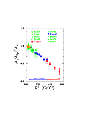
Figure 16: The ratio $\mu_{p}G_{Ep}/G_{Mp}$ from the two JLab experiments [Gay02, Pun05] (filled circle and square), together with all other polarization transfer experiments [Mil98, Gay01, Pos01, Die01, Str03, Hu06, MacL06, Jon06]. The systematic uncertainties apply to the JLab data only.

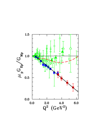
Figure 17: Comparison of $\mu_{p}G_{Ep}/G_{Mp}$ from the two JLab polarization data [Gay02, Pun05], and Rosenbluth separation; JLab Rosenbluth results from [Chr04, Qat05] shown as open, filled triangles, respectively. The rest of cross section data as in Figs. 6 and 6 (open circles). Dashed curve is a re-fit of Rosenbluth data [Arr03]; solid curve is the fit of Eq. (33).

The results from the two JLab experiments [Jon00, Pun05, Gay02] showed conclusively for the first time a clear deviation of the proton FF ratio from unity, starting at $Q^{2}\simeq 1$ GeV²; older data from [Ber71, Pri71, Bar73, Han73] showed such a decreasing ratio, but with much larger statistical and systematic uncertainties, as seen in Fig. 4. The most important feature of the JLab data, is the sharp decrease of the ratio $\mu_{p}G_{Ep}/G_{Mp}$ from 1 starting at $Q^{2}$ $\approx$ 1 GeV² to a value of $\sim 0.28$ at $Q^{2}$= 5.6 GeV², which indicates that $G_{Ep}$ falls faster with increasing $Q^{2}$ than $G_{Mp}$. This was the first definite experimental indication that the $Q^{2}$ dependence of $G_{Ep}$ and $G_{Mp}$ is different. If the $\mu_{p}G_{Ep}/G_{Mp}$-ratio continues the observed linear decrease with the same slope, it will cross zero at $Q^{2}\approx 7.5$ GeV² and become negative.

In Fig. 17 all the ratio data obtained from the Rosenbluth separation method are plotted together with the results of the two JLab polarization experiments. There are recent proton FF results obtained with the Rosenbluth separation method from two JLab experiments [Chr04, Qat05]; these results agree with previous Rosenbluth results [Lit70, Ber71, Pri71, Wal94, And94] and confirm the discrepancy between the ratios obtained with the Rosenbluth separation method and the recoil polarization method. The two methods give definitively different results; the difference cannot be bridged by either simple re-normalization of the Rosenbluth data [Arr03], or by variation of the polarization data within the quoted statistical and systematic uncertainties. This discrepancy has been known for the past several years and is currently the subject of intense discussion. A possible explanation is the hard two-photon exchange process, which affects both cross section and polarization transfer components at the level of only a few percents; however, in some calculations [Afa01, Blu03] the contribution of the two-photon process has drastic effect on the Rosenbluth separation results, whereas in others it does not [Bys06]; in either case it modifies the ratio obtained with the polarization method by a few percent only (this will be discussed in section 3.5). There are several experiments planned at JLab [Sul04, Arr05] to investigate the two-photon effects in the near future.

3.3.2 Neutron electric form factor measurements with polarization experiments

Measurements of the FFs of the neutron are far more difficult than for the proton, mainly because there are no free neutron targets. Neutron FF measurements were started at about the same time as for the proton, but the data are generally not of the same quality as for the proton, especially in the case of the electric FF of the neutron; the $Q^{2}$ range is limited also. The early measurements of the FFs of the neutron are discussed in sections 2.2.2 and 2.2.3; in this section we discuss only measurements made with longitudinally polarized electron beams on polarized ²H- or ³He-targets, and polarization transfer in the ²$H(\vec{e},e^{\prime}\vec{n})p$ reaction. We start with the measurements of the charge FF, $G_{En}$, and proceed then to the relatively few measurements of the magnetic FF, $G_{Mn}$.

The first measurement of the charge FF of the neutron, $G_{En}$, by the polarization method was made at MIT-Bates using the exclusive ²$H(\vec{e},e^{\prime}\vec{n})p$ reaction [Ede94]. The advantage of polarization measurements on the deuteron in the quasi free kinematics is that the extracted neutron FF is quite insensitive to the choice of deuteron wave functions, and also to higher order effects like final state interaction (FSI), meson exchange currents (MEC) and isobar configurations (IC), when the momentum of the knocked out neutron is in the direction of three-momentum transfer $\vec{q}$ [Are87, Rek89, Lag91].

For a free neutron the polarization transfer coefficient $P_{x}$ is given by Eq. (19). The relation between polarization transfer coefficient $P_{x}$, the beam polarization, $P_{e}$, and the measured neutron polarization component, $P^{\prime}_{x}$, is $P^{\prime}_{x}=P_{e}P_{x}$. The FF $G_{En}$ was extracted at a $Q^{2}$ of 0.255 GeV² in this experiment from the measured transverse polarization component $P^{\prime}_{x}$ of the recoiling neutron, and known beam polarization, $P_{e}$. This early experiment demonstrated the feasibility of extracting $G_{En}$ from the quasi-elastic ²$H(\vec{e},e^{\prime}\vec{n})p$ reaction with the recoil polarization technique, with the possibility of extension to larger $Q^{2}$ values.

Next, this same reaction ²$H(\vec{e},e^{\prime}\vec{n})p$ was used to determine $G_{En}$ at MAMI [Her99, Ost99] by measuring the neutron recoil polarization ratio $P_{x}/P_{z}$, at a $Q^{2}$ of 0.15 and 0.34 GeV². The ratio $P_{x}/P_{z}$ is related to $G_{E}/G_{M}$ as shown in Eq. (22). The measurement of the ratio, $P_{x}/P_{z}$, has some advantage, as discussed earlier for the proton, over the measurement of $P_{x}$ only, because in the ratio the electron beam polarization and the polarimeter analyzing power cancel; as a result the systematic uncertainty is small. In yet another experiment at MAMI the ratio of polarization transfer components, $P_{x}/P_{z}$, was measured using the same reaction ²$H(\vec{e},e^{\prime}\vec{n})p$ and the electric FF $G_{En}$ was obtained at $Q^{2}$ = 0.3, 0.6 and 0.8 GeV² [Gla05]; Glazier et al. concluded that their results were in good agreement with all other $G_{En}$ double-polarization measurements.

The experiment at JLab by Madey et al. [Mad03, Pla05] obtained the neutron FF ratios $G_{E}/G_{M}$ at $Q^{2}$ values of 0.45, 1.13 and 1.45 GeV² using the same method of measuring the recoil neutron polarization components $P_{x}$ and $P_{z}$ simultaneously, using a dipole with vertical B-field to precess the neutron polarization in the reaction plane, hence obtaining directly the ratio $G_{En}/G_{Mn}$. The best-fit values of $G_{Mn}$ were used to calculate values of $G_{En}$ from the ratio measurements. This is the first experiment that determined the value of $G_{En}$ with small statistical and systematic uncertainty and at the relatively high $Q^{2}$ values up to 1.45 GeV².

Passchier et al. [Pas99] reported the first measurement of spin-correlation parameters $A^{V}_{ed}$ at a $Q^{2}$ of 0.21 GeV² in ²$\vec{H}(\vec{e},e^{\prime}n)p$ reaction at NIKHEF; this experiment used a stored polarized electron beam and an internal vector polarized deuterium gas target; they extracted the value of $G_{En}$ from the measured sideways spin-correlation parameter in quasi-free scattering.

Experiment E93-026 at JLab extracted the neutron electric FF at $Q^{2}$ = 0.5 and 1.0 GeV² [Zhu01, War04] from measurements of the beam-target asymmetry using the ²$\vec{H}(\vec{e},e^{\prime}n)p$ reaction in quasi elastic kinematics; in this experiment the polarized electrons were scattered off a polarized deuterated ammonia (${ND_{3}}$) target. This experiment was the first to obtain $G_{En}$ at a relatively large $Q^{2}$ using a polarized target.

Blankleider and Woloshyn, in a paper in 1984 [Bla84], proposed that a polarized ³He target could be used to measure $G_{En}$ or $G_{Mn}$. They argued that the ³He ground state is dominated by the spatially symmetric S-state in which the two proton spins point in opposite directions, hence the spin of the nucleus is largely carried by the neutron. Therefore, the ³He target effectively serves as a polarized neutron target; and in the quasi-elastic scattering region the spin-dependent properties are dominated by the neutron in the ³He target.

There were experiments in the early 1990’s at MIT-Bates Laboratory that used a polarized ³He target and measured the asymmetry with polarized electrons in spin-dependent quasi-elastic scattering [Jon91, Tho92], and extracted the value of $G_{En}$ using the prescription of Blankleider and Woloshyn [Bla84], at a $Q^{2}$=0.16 and 0.2 GeV². However, Thompson et al. [Tho92] pointed out that significant corrections are necessary at $Q^{2}$=0.2 GeV² for spin-dependent quasi elastic scattering on polarized ³He according to the calculation of Laget [Lag91]; hence no useful information on $G_{En}$ could be extracted from these measurements; but Thompson et al. concluded that at higher $Q^{2}$ values the relative contribution of the polarized protons becomes significantly less and a precise measurements of $G_{En}$ using polarized ³He targets will become possible.

Starting in the early 1990’s, the neutron electric FF $G_{En}$ has been obtained in several experiments at MAMI, by measuring the beam-target asymmetry in the exclusive quasi-elastic scattering of electrons from polarized ${}^{3}He$ in the ³$\vec{He}(\vec{e},e^{\prime}n)pp$ reaction [Mey94, Bec99, Roh99, Ber03]. All the $G_{En}$ data from polarization experiments are shown in Fig. 19. In the first of these experiments, at MAMI, [Mey94], $G_{En}$ was obtained at $Q^{2}$ = 0.31 GeV². In following experiments at MAMI, $G_{En}$ was extracted at $Q^{2}$ of 0.35 GeV² [Bec99] and 0.67 GeV² [Roh99, Ber03] using the same reaction. The 0.35 GeV² point of [Bec99] was later corrected in [Gol01], based on Faddeev solutions and with some MEC corrections. The large effect of these corrections is illustrated in Fig. 19 with the dashed line connecting the open diamonds. The size of these corrections is expected to decrease with $Q^{2}$, although the corrections become increasingly difficult to calculate with increasing $Q^{2}$s.

Figure 18: Data for $G_{En}$ from beam asymmetry with polarized $D_{2}$ [Pas99, Zhu01, War04], and ³He [Mey94, Bec99, Roh99, Ber03], and recoil polarization with $D_{2}$ [Ede94, Her99, Ost99, Gla05, Pla05]. Included values obtained from $T_{20}$ [Abo99] in elastic $ed$, in [Schi01].

Figure 19: The data for $G_{Mn}$ from the two polarization experiments which have been performed so far, at Bates [Gao94] and JLab [And07], respectively.

3.3.3 Neutron magnetic form factor measurements with polarization experiments

Only two experiments have obtained the magnetic FF of the neutron, $G_{Mn}$, from polarization observables; both experiments used a polarized ³$\vec{He}$ target. The first experiment at the MIT-Bates laboratory, extracted $G_{Mn}$ from the measured beam-target asymmetry in inclusive quasi-elastic scattering of polarized electrons from polarized ³$\vec{He}$ target at $Q^{2}$ of 0.19 GeV² [Gao94]; the uncertainty on $G_{Mn}$ was dominated by the statistics, with a relatively small contribution from model dependence of the analysis. The second JLab experiment obtained $G_{Mn}$ for $Q^{2}$ values between 0.1 and 0.6 GeV², by measuring the transverse asymmetry in the ³$\vec{He}(\vec{e},e^{\prime})$ reaction in quasi-free kinematics [Xu00, Xu03, And07]. The values of $G_{Mn}$ were extracted in the plane wave impulse approximation (PWIA) at $Q^{2}$ of 0.3 to 0.6 GeV², and from a full Faddeev calculation at $Q^{2}$ of 0.1 and 0.2 GeV². The authors of this paper asserted that the PWIA extraction of $G_{Mn}$ is reasonably reliable in the $Q^{2}$ range of 0.3 to 0.6 GeV²; however, a more precise extraction of $G_{Mn}$ requires fully relativistic three-body calculations. The $G_{Mn}$ values from both experiments are shown in Fig. 19.

Figure 20: $G_{En}$ data as in Fig. 19, compared to the fits [Kel04] (thick line) and [Gal71] (thin solid line). Platchkov’s fits [Pla90] with 3 different $NN$ potentials shown as dotted [Rei68], dot-dashed [Lac81] and long dashes  [Wir84] lines, respectively.

Figure 21: The complete data base for $G_{Mn}$, from cross section and polarization measurements. Shown as a solid curve is the polynomial fit by Kelly [Kel04]; note that the recent data of  [Bro05] are not included in this fit.

3.4 Discussion of the form factor data

Probably the most important advance in the characterization of the FFs of the nucleon made in the last 10 years has been the realization that the so-called “scaling”-behavior of the proton FFs:

$$G_{Ep}\sim G_{Mp}/\mu_{p}~{}\sim~{}G_{D},$$ (32)

was limited to values of $Q^{2}$ smaller than 2 GeV². The recoil polarization data obtained at JLab in 1998 and 2000 proved beyond any doubt that for $Q^{2}$-values larger than 2 GeV², $G_{Ep}$ decreases faster than $G_{Mp}/\mu_{p}$ with a slope of -0.14 per GeV². What we now have are distinctly different $Q^{2}$-dependences for $G_{Ep}$ and $G_{Mp}$; in the $Q^{2}$ region investigated so far, the scaling-behavior is violated by a factor of 3.66 ${}^{+1.71}_{-0.88}$ at 5.54 GeV². The deviation of $G_{Ep}$ from the dipole FF is illustrated in Fig. 23, where only polarization results are shown. Of course it was well known that the dipole FFs, when Fourier transformed, produce unphysical distributions of charge or magnetization, with a discontinuity at zero radius. Nevertheless there were valid reasons, to believe that the dipole FF discussed in 2.2.4 may actually describe the FFs $G_{Ep}$, $G_{Mp}$ and $G_{Mn}$ of the nucleon. The data no longer support such expectations, as can be concluded by comparing the results in Figs. 6 and 23.

The discrepancy is related to the techniques used: all Rosenbluth separation of cross section data including the 2 new measurements from JLab [Chr04, Qat05] give $\mu_{p}G_{Ep}/G_{Mp}$ ratios close to the scaling behavior, except the early data shown in Fig. 3; all recoil polarization results for the same ratio are clustered along an approximately straight line versus $Q^{2}$, with a best fit valid above $Q^{2}\sim 0.4$ GeV² given by:

$$\mu_{p}G_{Ep}/G_{Mp}=1.0587-0.14265~{}Q^{2}.$$ (33)

A number of observations relative to this difference in results follows. First, there is one well established difference between the two techniques, cross section versus recoil polarization, and it is the relative importance of the radiative corrections required for them, as discussed in detail in section 3.5. The total radiative corrections as routinely calculated in cross section measurements is typically 10 to 30%, and the corrections are strongly $\epsilon$ dependent; this $\epsilon$ dependence affects primarily the results for $G_{Ep}^{2}$, and for increasing $Q^{2}$ the accuracy requirement for the correction becomes very demanding. Second, polarization observables, in recoil polarization or target asymmetry measurements, being ratios of cross sections, are only minimally affected by radiative corrections, and the ratio $G_{E}/G_{M}$ even less being a ratio of ratios. Nevertheless polarization data ultimately will require radiative corrections, particularly as experiments continue into the domain of yet larger $Q^{2}$. So is the discrepancy between Rosenbluth and polarization data entirely due to inaccuracy or incompleteness in the radiative correction? An immediate consequence of the previous statements is that radiative corrections for elastic $ep$ scattering in general have to be reexamined, as in their presently practiced form they are unable to reconcile the cross section results with polarization results.

Figure 22: Polarization data presented as $G_{Ep}/G_{D}$, where $G_{Ep}$ is obtained from the ratio $G_{Ep}/G_{Mp}$ obtained from polarization data in  [Pun05, Gay02, Cra06], multiplied by $G_{Mp}$ from the Kelly fit [Kel04].

Figure 23: The $G_{Mp}$ data were refitted in [Bra02] imposing the value of the $G_{Ep}/G_{Mp}$ from the recoil polarization data of Refs. [Pun05, Gay02], leaving out Rosenbluth separation data above 1 GeV².

Encouraging progress has been made including the one process certainly neglected in all previous radiative corrections, the exchange of two photons, neither one of them “soft” (this will be further discussed in section 3.5). Several calculations [Gui03, Afa05a, Blu03] suggest that this one diagram may contribute significantly to the $\epsilon$-dependence of the cross section; other considerations lead to the conclusion that the contribution from the two-photon term is too small at the $Q^{2}$-values of interest [Bys06], and/or leads to a definite non-linearity in the Rosenbluth plot which has not been seen in the data so far [Tom05].

Following the publication of the JLab recoil polarization $G_{Ep}/G_{Mp}$ ratios up to 5.54 GeV², the entire cross section data base for the proton has been reanalyzed by Brash et al. [Bra02], leaving all data above $Q^{2}=1$ GeV² out, using the data from [Jon00, Gay02] above this value of $Q^{2}$, and allowing for relative renormalization of all cross section data so as to minimize the $\chi^{2}$ of a global fit for $G_{Mp}$. The fitting function is the inverse of a polynomial of order 5. The renormalized values of $G_{Mp}$ show less scatter than the original data base, and the net effect of imposing the recoil polarization results is to re-normalize all $G_{Mp}$ data upward by 1.5-3% when compared with the older Bosted parametrization [Bos95], as shown in Fig. 23.

Another useful fit to the nucleon FFs which gives a good representation of the data is the one by Kelly [Kel04]. This fit uses ratios of polynomials with maximum powers chosen such that $G_{Ep}$, $G_{Mp}$ and $G_{Mn}$ have the asymptotic $1/Q^{4}$ behavior required by pQCD; in [Kel04] $G_{En}$ was also re-fitted with a Galster FF, as shown in Fig. 21.

In Figs. 21 and 21 we compare all the data available for $G_{En}$ and $G_{Mn}$, obtained from cross section and polarization observables. The $G_{En}$ data obtained in double polarization show reasonable consistency above 0.5 GeV²; they are systematically higher than the older cross section results shown in Fig. 21 by the 3 Platchkov fits [Pla90]. The revision by Kelly [Kel04] of the Galster fit [Gal71] gives an excellent representation of the data available today.

Recently, more and better data have been obtained for $G_{En}$, exclusively by the polarization method, either recoil polarization transfer or target asymmetry, with deuterium and ³He targets and up to $Q^{2}$=1.5 GeV². No drastic change of the general behavior of $G_{En}$ has been observed to this point in time. There is a new measurement of $G_{En}$ at JLab up to a $Q^{2}$ of 3.4 GeV² [Cat03], but the data have yet to be analyzed. In general all polarization data for $G_{En}$ have given results larger than those obtained from elastic scattering; these earlier data required considerable nuclear structure corrections, as illustrated in Fig. 19; the sensitivity to the deuteron wave function, therefore to the $NN$ potential used, was extensively discussed at the time in  [Pla90].

The data for $G_{Mn}$ come mostly from cross section measurements, except two polarization measurements, using polarized ³He target, one at MIT-Bates for low $Q^{2}$ with large uncertainty [Gao94] and the other a recent measurement at JLab [Xu00, Xu03, And07]. The most recent Hall B results [Bro05], which extend to $Q^{2}$ of nearly 5 GeV², and used quasi-elastic scattering on deuterium, reveal some internal inconsistency in the data base near 1 GeV² as shown in Fig. 21; as can be seen in Fig. 21 there is some disagreement between the results of different experiments in the $Q^{2}$ range of 0.3 to 1.5 GeV². . These measurements will be extended to 14 GeV² after the JLab upgrade to 12 GeV; similarly, the measurement of $G_{Ep}/G_{Mp}$ will be continued to 13 GeV² after the upgrade.

Several experiments are planned at JLab to resolve the dichotomy in the $G_{Ep}/G_{Mp}$ ratio. One experiment will measure the ratio of the $e^{-}p$ and $e^{+}p$ cross sections, which determines directly the real part of the two-photon amplitude [Afa04]. Another experiment will measure the ratio $G_{Ep}/G_{Mp}$ at fixed Q²=2.5 GeV² [Sul04], as a function of $\epsilon$, to detect the two hard photon contribution as a variation of this ratio; non constancy would be related to the real part of the two-photon amplitude. A third experiment will be a high statistics search of non-linearity in the Rosenbluth plot in $ep$-scattering, which should also reveal the contribution of the two-photon process ([Arr05]). Measurements of the induced polarization in ${e}p\rightarrow{e}\vec{p}$ (a byproduct of the experiment from [Sul04]) , and of the single spin target asymmetry in quasi elastic scattering on the neutron in ${}^{3}{He}^{\uparrow}({e},{e}^{\prime})$ for target polarization normal to the reaction plane [Ave05], will measure the imaginary part of the two-gamma contribution. The transverse beam spin asymmetry in $ep$ has been measured at Bates [Wel01] and MAMI [Maa05]; it too originates from the imaginary part of the two-photon contribution.

3.5 Rosenbluth results and radiative corrections

All cross section measurements have been single arm experiments, $(e,e^{\prime})$, except three early experiments at Cambridge [Pri71, Han73] and DESY [Bar73] in which both proton and electron were detected, $(e,e^{\prime}p)$, and the most recent one of Qattan et al. [Qat05], in which only the proton was detected, $(e,p)$. In all cases, measured raw cross sections need to be corrected for QED processes to first order in $\alpha\sim 1/137$, before accessing the cross section corresponding to one-photon-exchange, or Born term. Only to the extent that these corrections remain relatively small, can one hope to obtain the Born term FFs $G_{E}^{2}$ and $G_{M}^{2}$, which are functions of $Q^{2}$ only, using the Rosenbluth method.

The effect of the radiative correction on the cross section is typically in the range 10-30%; what is important however, is the fact that overall, the radiative corrections are $\epsilon$-dependent; i.e. they affect the slope of the Rosenbluth plot. Although radiative corrections have been applied to all data taken after 1966 using the “recipe” of Tsai [Tsa61], Mo and Tsai [MoT69] and [Tsa71], not all corrections were applied in all data sets. This point was recently reviewed by Arrington [Arr03], who reanalyzed some of the cross section data; the fit to the re-analyzed data is included in Fig. 17. Furthermore, in the references [Tsa61, MoT69, Tsa71] the effect of the structure of the nucleon was ignored, and a number of approximations were made. In more recent work on radiative corrections, Maximon and Tjon [Max00] have included the structure of the proton by introducing the proton FF, and they also eliminated some of the soft-photon approximations made by [Tsa61, MoT69, Tsa71]. In the current energy range of JLab, the difference for $\delta$, the radiative correction, used in $\frac{d\sigma}{d\Omega}=(1+\delta)\frac{d\sigma^{Born}}{d\Omega}$ up to corrections of order $\alpha^{3}$, between the older and the new calculation is at the level of several %.

The various internal radiative correction diagrams involving the electron are shown in Fig. 25. The first order virtual radiative processes are the vertex diagram b), the photon self-energy diagram c) and the two self-energy diagrams for the electron d); the first order real radiative processes include emission of a real photon by either the initial or the final electron diagram e). Similarly diagrams for the proton include bremsstrahlung a), vertex b) and proton self energy c), shown in Fig. 25. Two-photon exchange is shown as diagram e). In addition there are external radiative corrections due to the emission of real photons by the incoming and scattered electrons in the material of the target, as well as energy loss by ionization.

Figure 24: Born term and lowest order radiative correction graphs for the electron in elastic $ep$.

Figure 25: Lowest order radiative correction for the proton side in elastic $ep$ scattering.

The virtual part of the internal radiative corrections depend exclusively upon $Q^{2}$, thus it generates no $\epsilon$-dependence, hence does not modify the value of $G_{Ep}^{2}$, but modifies the value of $G_{Mp}^{2}$ directly.

The radiative correction for real photon emission (bremsstrahlung) is energy, and therefore $\epsilon$ dependent, and it also results in a changed value of $Q^{2}$. In general the scattered electron energy spectrum is integrated up to a maximum energy loss which is kept below the pion threshold. The correction is different for different experiments; it depends on the procedure used to integrate over the scattered electron energy, or missing mass squared spectrum.

The contributions due to real photon emission by the initial and final proton, as well as the proton vertex and two-photon exchange with one soft- and one hard photon are relatively small, but strongly $\epsilon$-dependent.

The external part of the radiative corrections includes only real photon emission by the incident and scattered electron, and is not coherent with the $ep$ interaction. Although the correction for the incoming electron in the target is energy independent, and it can be averaged to a value at the center of the active area of the target for all kinematics of a given experiment, the correction for the scattered electron in the target depends directly upon the target length and diameter which determines the amount of target material traversed, and therefore the scattering angle. As the desired range of $\epsilon$ values is obtained by changing the electron scattering angle, this correction has $\epsilon$-dependence. For the data of Andivahis et al. [And94] the external corrections are one fourth to one half as large as the internal corrections from the smallest to the largest $\epsilon$-values as shown in Fig. 28. The calculation of the external correction requires information on the spectrometer acceptance and on the target geometry, and is an integral part of the analysis of the data; it cannot be repeated on the basis of published data. However, it is potentially a significant source of uncertainty in the $\epsilon$-dependence of the total radiative correction.

Figure 26: The various contributions to the correction factor $\delta$ at $Q^{2}$=5 GeV², calculated with the code from [Vdh00] based on the work of Maximon and Tjon [Max00], including the external correction for a 15 cm target, taken from [And94].

Figure 27: Rosenbluth plot for data of et al. [And94]. At bottom before radiative correction, at top after radiative correction. Filled squares, triangles and circles for 1.75, 3.25 and 5 GeV², respectively; empty symbols for uncorrected data.

Figure 28: The $Q^{2}$= 5 GeV² data of [And94], with their best fit (thick solid line), compared with the results of the various calculations of the radiative correction, taken from Refs. [Vdh00, Afa05a, Bys06]. Also shown is the slope from the JLab polarization data.

To gain some appreciation of what term might be most strongly affecting the final result of the radiative correction, we show the values $\delta_{real}+\delta_{virtual}$, graphs b), c), d) and e) in Fig. 25, $\delta_{12}$ from graphs a), b),c) and d) in Fig. 25, and $\delta_{external}$ for the condition of the Andivahis experiment [And94] separately in Fig 28. The curve in Fig. 28 labeled $\delta_{int+ext}$ determines the overall correction. Its slope versus $\epsilon$ is due to the combined effect of the real and external-contributions, with the proton contribution reducing it somewhat; $\delta_{virtual}$ has no $\epsilon$-dependence.

The importance of calculating the contributions to the radiative correction which are $\epsilon$-dependent accurately is illustrated in Fig. 28. Shown in this figure are reduced cross sections defined in terms of the $(\frac{d\sigma}{d\Omega})_{reduced}$ from Eq. (13) as:

$$\sigma_{R}=\left(\frac{d\sigma}{d\Omega}\right)_{reduced}/G_{D}^{2}=\frac{\epsilon}{\tau}\frac{G_{E{p}}^{2}}{G_{D}^{2}}+\frac{G_{M{p}}^{2}}{G_{D}^{2}},$$ (34)

as a function of $\epsilon$ for the data of Andivahis et al. [And94]. If both FFs are functions of $Q^{2}$ only, the intercept of a straight line fit is $G_{M{p}}^{2}/G_{D}^{2}\sim\mu_{p}^{2}$, and the slope is $\frac{1}{\tau}\frac{G_{E{p}}^{2}}{G_{D}^{2}}$. Most noticeable in this figure is the negative slope of the uncorrected data, above $Q^{2}$=3 GeV². This figure dramatically illustrates the importance of the radiative correction and gives a measure of the accuracy that is required to obtain the FFs with the desired accuracy. The final value of $G_{Ep}^{2}$ obtained from cross section data depends directly upon the value and the accuracy of the $\epsilon$-dependent part of the radiative correction. Note that the radiative corrections for the data of [And94] were made following Mo and Tsai [Tsa61, MoT69, Tsa71], with the additional corrections introduced in Ref. [Wal94].

More recently Maximon and Tjon [Max00] have reconsidered the radiative correction calculation, and included additional terms with explicit emphasis of the hadronic effects. A similar reexamination of the Mo-Tsai procedure was made by Vanderhaeghen et al. [Vdh00] in the process of a detailed calculation of radiative corrections for virtual Compton (VCS). Also recently Ent et al. [Ent01] and Weissbach et al. [Wei04] have published improvements and detailed studies of the radiative correction calculation technique for coincidence experiments (e,e’p).

Most recently Bystritskiy et al. [Bys06] have calculated the radiative corrections for elastic $ep$ scattering using the Drell-Yan electron structure function approach; no co-linearity approximation is made in such a calculation, but the proton vertex corrections have not been included so far; the diagram with two hard photons has been approximatively calculated using both nucleon and $\Delta$ intermediate states and was found to make a negligible contribution. The results of [Bys06] suggest that hard bremsstrahlung may cause the difference between the Rosenbluth and polarization results. Usual bremsstrahlung calculations are for soft bremsstrahlung, where the emitted photon energy is kept only to linear order in denominators and entirely omitted in numerators. Soft bremsstrahlung multiplies all amplitudes by the same factor and does not, for a relevant example, change the slope on a Rosenbluth plot. If one makes no approximations in the photon energy, there can be different effects on different spin amplitudes. Thus the claim is that emitted photons that are energetic enough to affect the spin structure of the calculation but still small enough to escape detection, give rise to the difference between the two methods of measuring $G_{Ep}/G_{Mp}$. A contrasting numerical claim is that hard bremsstrahlung effects are noticeable and helpful in reconciling the Rosenbluth and polarization experiments, but are not decisive, see Ref. [Afa05b]. These contrasting claims clearly need to be sorted out, but an independent reexamination is not available as of this writing.

The effect of these new radiative corrections is illustrated in Fig. 28. The dashed-dot line is obtained from the $Q^{2}$=5 GeV², uncorrected data from [And94], applying the radiative correction calculated with the code of [Vdh00], with the same energy cuts as used in the original data. This correction is 2.5% smaller than the one in [And94] at $\epsilon$=1. The two-photon calculation result shown is obtained by removing the soft part of the two-photon contribution, and replacing it by the GPD based calculation of [Afa05a]; the result is then refitted with a straight line (dotted line). The resulting value at $\epsilon$=1 is 4.5% smaller than the original correction. The long dashed line represents the results of [Bys06], after correcting the experimental data points [Tom06], using the same energy cuts as in the data, and refitting with a straight line (dashed line); these results are almost identical to the ones obtained with two-photon correction [Afa05a]. The slope calculated from the fit to the JLab recoil polarization data, for $Q^{2}$=5 GeV², from Eq. (33), is shown as the short dashed line. The value at $\epsilon$=1 is 6% smaller than that of the original Rosenbluth data of Ref.[And94]. In Fig. 28 all fits are drawn with a renormalized value of $\sigma_{R}$ at $\epsilon$=0, to emphasize the differences in slope, which determine $G_{Ep}$; based on the recoil polarization results the contribution of $G_{Ep}$ to the cross section at $Q^{2}$=5 GeV² is $\sim$1%.
All three corrections are different, and each one of them brings the Rosenbluth results closer to the recoil polarization results, indicating that present uncertainties in the calculations of the radiative corrections of the cross section are at the level of several %s.
In [Arr04], the effect of the Coulomb distortion of the incoming and outgoing electron waves on the extraction of the proton FFs was studied. Coulomb distortion corresponds to the exchange of one hard and one (or several) soft photons. It was found that it does yield an $\epsilon$ dependent correction to the elastic electron-proton cross sections. Although it reduces the cross sections, its magnitude is too small to explain the discrepancy between Rosenbluth and polarization methods. It is however straightforward to calculate and should be included in the data analysis.
Following the important discrepancy between the determinations of $G_{Ep}/G_{Mp}$ using the polarization transfer and Rosenbluth techniques, the role of two hard photon exchange effects, beyond those which have already been accounted for in the standard treatment of radiative corrections has been studied. A general study of two- (and multi)-photon exchange contributions to the elastic electron-proton scattering observables was given in [Gui03]. In that work, it was noted that the interference of the two-photon exchange amplitude with the one-photon-exchange amplitude could be comparable in size to the $(G_{Ep})^{2}$ term in the unpolarized cross section at large $Q^{2}$. In contrast, it was found that the two-photon exchange effects do not impact the polarization-transfer extraction of $G_{Ep}/G_{pM}$ in an equally significant way. Thus a missing and un-factorisable part of the two-photon exchange amplitude at the level of a few percent may well explain the discrepancy between the two methods.
Realistic calculations of elastic electron-nucleon scattering beyond the Born approximation are required in order to demonstrate in a quantitative way that $2\gamma$ exchange effects are indeed able to resolve this discrepancy.
Recently, several model calculations of the $2\gamma$ exchange amplitude have been done. In  [Blu03], a calculation of the $2\gamma$ exchange when the hadronic intermediate state is a nucleon was performed. It found that the $2\gamma$ exchange correction with intermediate nucleon can partially resolve the discrepancy between the two experimental techniques. However, subsequently it was found in  [Kon05] that the effect is partly canceled when including the next hadronic intermediate state, the $\Delta(1232)$ resonance. The $2\gamma$ exchange contribution to elastic $eN$ scattering has also been estimated at large momentum transfer [Che04, Afa05a], through the scattering off a parton in a proton by relating the process on the nucleon to the generalized parton distributions. This approach effectively sums all possible intermediate states corresponding to excitations of the nucleon . Applying the two-photon exchange corrections to the unpolarized data (see dotted curve in Fig. 28), yields a much flatter slope for the Rosenbluth plot, hence a much smaller value of $G_{E}$. The two-photon exchange corrections to the Rosenbluth process can therefore substantially reconcile the two ways of measuring $G_{E}/G_{M}$ (compare dotted with thin solid curves in Fig. 28).
To push the precision frontier further in electron scattering, one needs a good understanding, of $2\gamma$ exchange mechanisms, and of how they may or may not affect different observables. This justifies a systematic study of such $2\gamma$ exchange effects, both theoretically and experimentally. Experimentally, the real part of the $2\gamma$ exchange amplitude can be accessed through the difference between elastic electron and positron scattering off a nucleon. Such experiments are planned in the near future.

To conclude, on the one hand the discussion above makes it clear that the radiative corrections, including two hard photon exchange, for the cross section data are not complete at this point in time. Therefore, the FFs $G_{E}^{2}$ and $G_{M}^{2}$ obtained using the Rosenbluth method above $Q^{2}$ of 2 GeV² are not correct. On the other hand, all the authors cited above agree that radiative corrections change the longitudinal and transverse polarization components, $P_{t}$ and $P_{\ell}$, in $\vec{e}+p\rightarrow{e}+\vec{p}$, similarly, with the ratio $P_{t}/P_{\ell}$ affected only at the level of a few percent. The radiative corrections specifically calculated for the JLab polarization data by Afanasev et al. [Afa01] found that the corrections are $\sim$1%, whereas the hard two photon exchange effects are at the few percent level [Che04, Afa05a]. Hence the polarization transfer method gives correct values for the FFs.

4 Theoretical interpretation of nucleon electromagnetic form factors

In this section we give an overview of the theoretical understanding of the nucleon e.m. FFs. These FFs encode the information on the structure of a strongly interacting many-body system of quarks and gluons, such as the nucleon. This field has a long history and many theoretical attempts have been made to understand the nucleon FFs. This reflects the fact that a direct calculation of nucleon FFs from the underlying theory, Quantum Chromodynamics (QCD), is complicated as it requires, in the few GeV momentum transfer region, non-perturbative methods. Hence, in practice it involves approximations which often have a limited range of applicability. Despite their approximations and limitations, some of these non-perturbative methods do reveal some insight in the nucleon structure.
The earliest models to explain the global features of the nucleon FFs, such as its approximate dipole behavior, were vector meson dominance (VMD) models which are discussed in Sect. 4.1. In this picture the photon couples to the nucleon through the exchange of vector mesons. Such VMD models are a special case of more general dispersion relation fits, which allow to relate time-like and space-like FFs, and which are discussed subsequently.
To understand the structure of the nucleon in terms of quark and gluon degrees of freedom, constituent quark models have a long history. We discuss the intricacies in describing a bound system of relativistic constituent quarks and review the resulting predictions for FFs in Sect. 4.2. Despite some of their successes, models based on quarks alone do suffer from the evident shortcoming that they do not satisfy the global chiral symmetry of QCD when rotating left and right handed light quarks in flavor space. This chiral symmetry is broken spontaneously in nature, and the resulting Goldstone bosons are pions. Since they are the lightest hadrons, they dominate the low momentum transfer behavior of form factors, and manifest themselves in a pion cloud surrounding the nucleon. Such pion cloud models will also be discussed in Sect. 4.2.
In Sect. 4.3, we discuss the spatial information which can be obtained from the nucleon FFs, and discuss both radial densities and the issue of shape of the nucleon.
Sect. 4.4 describes the chiral effective field theory of QCD and their predictions for nucleon FFs at low momentum transfers, where such perturbative expansions are applicable.
In Sect. 4.5, we shall discuss the lattice QCD simulations, which have the potential to calculate nucleon FFs from first principles. This is a rapidly developing field and important progress has been made in the recent past. Nevertheless, the lattice calculations are at present still severely limited by available computing power and in practice are performed for quark masses sizably larger than their values in nature. We will discuss the issues in such calculations and compare recent results. It will also be discussed how the chiral effective field theory can be useful in extrapolating present lattice QCD calculations to the physical pion mass.
In Sect. 4.6, we discuss the quark structure of the nucleon and discuss generalized parton distributions (GPDs) of the nucleon. These GPDs are being accessed in hard exclusive reactions, which allow to remove in a controlled way a quark from the initial nucleon and implanting instead another quark in the final nucleon. The resulting GPDs can be interpreted as quark correlation functions and have the property that their first moments exactly coincide with the nucleon FFs. We discuss the information which has been obtained on GPDs from fits of their first moments to the precise FF data set.
Finally, in Sect. 4.7, we discuss the nucleon FFs in the framework of perturbative QCD. These considerations are only valid at very small distances, where quarks nearly do not interact. In this limit, the nucleon FFs correspond to a hard photon which hits a valence quark in the nucleon, which then shares the momentum with the other (near collinear) valence quarks through gluon exchange. We discuss the predictions made in this limit and confront them with the experimental status for Dirac and Pauli FFs at large momentum transfers.

4.1 Dispersion theory

4.1.1 Vector Meson Dominance (VMD)

The starting point in understanding the interaction of a vector probe such as the photon with a hadronic system is provided by the observation that the lowest lying hadrons with vector quantum numbers are the vector mesons $\rho(770)$, $\omega(782)$ and $\phi(1020)$. In the process $e^{+}e^{-}\to hadrons$, these vector mesons show up as prominent resonances at the corresponding values of the $e^{+}e^{-}$ squared $c.m.$ energy $q^{2}>0$. One therefore expects that in the elastic electron scattering process on the nucleon, $eN\to eN$, the nucleon electromagnetic FFs at low space-like momentum transfers, $q^{2}<0$, will be dominated by these lowest lying singularities from the time-like region. A large class of models for $F_{1}$ and $F_{2}$ are based on this vector meson dominance (VMD) hypothesis, as depicted in Fig. 29.

Figure 29: The vector meson dominance picture for the coupling of the photon (with four-momentum $q$) to a nucleon.

Within such VMD models, the approximate dipole behavior of the nucleon e.m. FFs, see Eq. (14), can be understood as being due to the contribution of two nearby vector meson poles which have opposite residua. Assume that one considers two vector meson pole contributions in Fig. 29 (with masses $m_{V1}$ and $m_{V2}$ and residua of equal magnitude and opposite sign $a$ and $-a$ respectively), one obtains :

$$F_{1,2}(q^{2}) \sim \frac{a}{q^{2}-m_{V1}^{2}}+\frac{(-a)}{q^{2}-m_{V2}^{2}}=\frac{a\,(m_{V1}^{2}-m_{V2}^{2})}{(q^{2}-m_{V1}^{2})(q^{2}-m_{V2}^{2})}.$$ (35)

An early VMD fit was performed by Iachello et al. [Iac73] and predicted a linear decrease of the proton $G_{Ep}/G_{Mp}$ ratio, which is in basic agreement with the result from the polarization transfer experiments. Such VMD models have been extended by Gari and Krümpelmann [Gar85] to include the perturbative QCD (pQCD) scaling relations [Lep80], which state that (see Sect. 4.7) $F_{1}\sim 1/Q^{4}$, and $F_{2}/F_{1}\sim 1/Q^{2}$.
In more recent years, extended VMD fits which provide a relatively good parameterization of all nucleon e.m. FFs have been obtained. An example is Lomon’s fit [Lom01], using $\rho(770)$, $\omega(782)$, $\phi(1020)$, and $\rho^{\prime}(1450)$ mesons and containing 11 parameters. Another such recent parameterization by Bijker and Iachello [Bij04] including $\rho(770)$, $\omega(782)$, and $\phi(1020)$ mesons only achieves a good fit by adding a phenomenological contribution attributed to a quarklike intrinsic $qqq$ structure (of $rms$ radius $\sim 0.34$ fm) besides the vector-meson exchange terms. The pQCD scaling relations are built into this fit which has 6 free parameters which are fit to the data. In contrast to the early fit of Ref. [Iac73], the new fit of Ref. [Bij04] gives a very good description of the neutron data, albeit at the expense of a slightly worse fit for the proton data.
It will be interesting to check the resulting VMD fits for the neutron FFs to larger $Q^{2}$. In this regard, an interesting “prediction” can be drawn when the FFs $F_{2}$ and $F_{1}$ obtained directly from double polarization experiments are shown in the same graph for the proton and the neutron, as in Fig. 30. It is remarkable that both $F_{1}$ and $F_{2}$ tend toward the same value for proton and neutron, and may meet at a $Q^{2}$ value which will soon be accessible for the neutron. This conclusion is influenced by the VMD fits shown in the same figure, and rests on their extrapolation for the neutron to larger $Q^{2}$. Note that the VMD fits shown include all data for p and n, but selects the recoil polarization over the Rosenbluth results for $Q^{2}$ larger than 1 GeV².

Figure 30: The FFs $F_{1}$ and $F_{2}$ for the proton and the neutron obtained from double polarization experiments only. The values of $F_{2}$ and $F_{1}$ were obtained from the experimental FF ratios using fitted values to the data base for $G_{Mp}$ and $G_{Mn}$. For the proton data, the fit from [Kel04] was used; for the neutron data in [Mad03] the fit from [Kel04], and in [War04] the fit from [Kub02] were used. The curves are the VMD fits of Lomon [Lom01] and of Bijker and Iachello [Bij04].

4.1.2 Dispersion analyses

Despite the relatively good fits obtained by the VMD models, it was already pointed out in 1959 by Frazer and Fulco [Fra59] that such an approach is at odds with general constraints from unitarity. Assuming an unsubtracted dispersion relation (DR), the nucleon e.m. FFs $F(q^{2})$, where $F$ generically stands for any of the four FFs, can be obtained as :

$$F(q^{2})=\frac{1}{\pi}\int_{t_{0}}^{\infty}\,dq^{\prime\,2}\,\frac{\mathrm{Im}F(q^{\prime\,2})}{q^{\prime\,2}-q^{2}}.$$ (36)

The dispersion analyses are performed separately for nucleon isoscalar and isovector FFs. In the vector-isovector spectral function $\mathrm{Im}F(q^{\prime\,2})$ one notices a large non-resonant contribution starting from $t_{0}=4m_{\pi}^{2}$ and extending under the $\rho$-peak. Such a non-resonant contribution arises due to the two-pion continuum. For the isoscalar spectral function, the integral starts at $t_{0}=9m_{\pi}^{2}$, corresponding to $3\pi$ intermediate states. The two-pion continuum contribution was estimated by Höhler and collaborators [Hoh76] by using pion time-like FF data and $\pi\pi\to N\bar{N}$ amplitudes which were determined by extrapolating $\pi N$ partial waves to the time-like region [Hoh75].
Höhler’s analysis has been updated by Mergell, Meissner, and Drechsel [Mer96] in the mid-nineties and extended to include the nucleon time-like FF data [Ham96]. The inclusion of recent neutron FF data in such dispersion relation analysis has been performed in Ref. [Ham04]. The resulting analysis describes the nucleon isovector FFs through the $2\pi$ continuum (including the $\rho(770)$), and three additional vector isovector meson poles : $\rho^{\prime}(1050)$, $\rho^{\prime\prime}(1465)$, $\rho^{\prime\prime\prime}(1700)$. The isoscalar FFs are described by four vector isoscalar meson poles : $\omega(770)$, $\phi(1020)$, $S^{\prime}(1650)$ and $S^{\prime\prime}(1680)$. In this approach, the masses of the mesons $\rho^{\prime}$, $\rho^{\prime\prime}$, $\rho^{\prime\prime\prime}$, $S^{\prime},S^{\prime\prime}$ and the 14 residua (one for both the vector ($F_{1}$) and tensor ($F_{2}$) channels for each meson) are fitted and the pQCD scaling behavior is parameterized through three additional parameters. Note that for the isovector channel, the fitted masses for $\rho^{\prime\prime}$ and $\rho^{\prime\prime\prime}$ correspond to physical particles listed by the Particle Data Group (PDG), whereas enforcing the correct normalization of all FFs, the experimental value for the neutron charge radius, as well as the pQCD scaling behavior, requires the inclusion of an unphysical $\rho^{\prime}$ meson with mass 1050 MeV. The analysis of Hammer and Meissner [Ham04] also finds that the residua for both isovector FFs $F_{1}^{V}$ and $F_{2}^{V}$ of $\rho^{\prime\prime}$ and $\rho^{\prime\prime\prime}$ are relatively close in magnitude and opposite in sign, required by the approximate dipole behavior of the isovector FFs. For the isoscalar FFs $F_{1}^{S}$ and $F_{2}^{S}$, the fit also drives the residua of the nearby poles $S^{\prime}$ and $S^{\prime\prime}$ to values very close in magnitude and of opposite signs, required by the approximate dipole behavior of the isoscalar FFs. Using such an analysis, a good description of most FF data with the exception of the $G_{Ep}/G_{Mp}$ polarization data at $Q^{2}>3$ GeV², was obtained in [Ham04].

Figure 31: Dispersion relation (15 parameter) fit for the four nucleon (space-like) e.m. FFs compared with the world data (circles) including the JLab/CLAS data for $G_{Mn}$ (triangles) [Bro05]. The dashed curves indicate the $1\sigma$ deviation from the fit, given by the solid curves. Figure from Ref. [Bel07].

The dispersion relation analysis of nucleon e.m. FFs has been further improved by Belushkin et al. [Bel07]. In addition to the $2\pi$ continuum present in the isovector spectral functions of the previous DR analyses, also the $\rho\pi$ and $K\bar{K}$ continua were included as independent input in the isoscalar spectral functions. In Ref. [Bel07], the $2\pi$ continuum was reevaluated using the latest experimental data for the pion FFs in the time-like region [Bel06]. The $K\bar{K}$ continuum was obtained from an analytic continuation of $KN$ scattering data [Ham99]. Following the work of Ref. [Mei97], the $\rho\pi$ continuum was approximated in the DR analysis by an effective pole term for a fictitious $\omega^{\prime}$ meson with mass : $m_{\omega^{\prime}}=1.12$ GeV. This approximate $\rho\pi$ continuum is found to yield an important negative contribution to $F_{1}^{S}$. The remaining contributions to the spectral functions are parameterized by vector meson poles from a fit to the FF data. The parameters in the fit were constrained to yield the correct normalization of the FFs at zero momentum transfers. The asymptotic constraints from pQCD were included in two different forms : either as a superconvergence relation or by adding an explicit continuum term with the imposed pQCD behavior. A simultaneous fit to the world data for all four FFs in both the space-like and time-like regions was performed. Fig. 31 shows this fit for the nucleon space-like FFs where for $G_{Ep}/G_{Mp}$ at larger $Q^{2}$ the JLab/Hall A polarization data [Jon00, Gay02, Pun05] have been used, and where for $G_{Mn}$ the preliminary JLab/CLAS data [Bro05] have been included. In this fit, the pQCD limit was imposed through an explicit continuum term and the minimum number of poles in addition to the $\pi\pi$, $\rho\pi$ and $K\bar{K}$ continua were chosen to fit the data. In addition to the $\omega(782)$, the fit yields two more isoscalar poles ($m_{s1}\simeq 1.05$ GeV and $m_{s2}\simeq 1.4$ GeV), and three additional isovector poles ($m_{v1}\simeq 1.0$ GeV, $m_{v2}\simeq 1.6$ GeV, and $m_{v3}\simeq 1.8$ GeV ). The resulting 15 parameter fit shown in Fig. 31 has a total $\chi^{2}$/d.o.f. value of 2.2.
It will be interesting to confront the most recent and sophisticated DR fit of [Bel07] with upcoming data for $G_{Ep}/G_{Mp}$ out to 8.5 GeV² [Bra04]. In all discussed VMD and DR fits starting with Gari-Krümpelmann [Gar85] the asymptotic pQCD limit $F_{2}/F_{1}\sim 1/Q^{2}$ was built in, although the data do not support this limit at available momentum transfers, see Fig. 43 in Sect. 4.7. Besides, there is various theoretical work indicating that the pQCD prediction, in particular for $F_{2p}$, might only set in at significantly larger values of $Q^{2}$, of the order of several tens of GeV². It might therefore be worthwhile to investigate how the DR analysis changes by removing the bias $F_{2}/F_{1}\sim 1/Q^{2}$ from the analysis, when fitting data in the range up to $Q^{2}\sim 10$ GeV².

4.2 Quark models versus pion-cloud models

4.2.1 Constituent quark models

In our quest to understand the structure of the nucleon in terms of the quark and gluon degrees of freedom which appear in the QCD Lagrangian, constituent quark models (CQMs) have a long history, which predates the establishment of the theory of strong interactions, QCD. In a CQM, the nucleon appears as the ground state of a quantum-mechanical three-quark system in a confining potential. In such a picture, the ground state baryons (composed of the light up ($u$), down ($d$) and strange ($s$) quark flavors) are described by $SU(6)$ spin-flavor wave functions (WFs), supplemented by an antisymmetric color WF.
In the Isgur-Karl model [Isg78], the constituent quarks move in a harmonic oscillator type confining potential. For the ground state baryons, the three constituent quarks are in the $1s$ oscillator ground state, corresponding to the [56]-plet of $SU(6)$. In the Isgur-Karl model, the long-range confining potential is supplemented by an interquark force corresponding to one-gluon exchange. The one-gluon exchange leads to a color hyperfine interaction between quarks, which breaks the $SU(6)$ symmetry and leads to a mass splitting between $N(939)$ and $\Delta(1232)$, often referred to as the hyperfine splitting. It was found that it also predicts well the mass splittings between octet and decuplet baryons [DeR75]. Furthermore, the color hyperfine interaction leads to a tensor force which produces a small $D$-state ($L=2$) admixture in the $N$ (as well as $\Delta$) ground states [Kon80, Isg82], corresponding to a $D$-state probability in the $N$ ground state around 0.2 %. Even though such $D$-wave probability is small, it leads to a non-spherical charge distribution. For a static charge distribution, a measure of the non-sphericity (or deformation) is given by its quadrupole moment. Since the nucleon has spin 1/2, an intrinsic quadrupole moment of the nucleon cannot be directly measured because angular momentum conservation forbids a non-zero matrix element of a ($L=2$) quadrupole operator between spin 1/2 states. However this quadrupole deformation may reveal itself in an electromagnetically induced transition from the spin 1/2 $N$ to the spin 3/2 $\Delta$ state. In this way, the tensor force between quarks gives rise to non-zero values for the electric quadrupole ($E2$) and Coulomb quadrupole ($C2$) transitions.
The non-relativistic CQM, despite its simplicity, is quite successful in predicting the spectrum of low-lying baryons, and gives a relatively good description of static properties such as the octet baryon magnetic moments. To calculate the FFs of a system of constituents with masses small compared with the confinement mass scale necessitates however a relativistic treatment even for low momentum transfers. For momentum transfers several times the nucleon mass squared a relativistic description becomes crucial.
In contrast to the calculation of the spectrum, which uses eigenfunctions of a Poincaré invariant mass operator, a calculation of the nucleon electromagnetic FFs requires the relation between the rest frame spin and momenta (in the three-quark WF) and those in the moving frame. This requires an extension of eigenfunctions of the spin and mass operators, so as to transform consistently under the unitary representations of the Poincaré group. The way to implement relativity into a Hamiltonian formalism (describing e.g. a system of three interacting constituent quarks) has been laid out by Dirac [Dir49]. There are three forms of dynamics (so called instant, point, and light-front forms) which differ in the choice of the kinematical subgroup of the Poincaré group. This is the subgroup of the Poincaré group whose commutator relations are not affected by the interactions between the constituents. The three (unitarily equivalent) forms therefore differ by which of the ten generators of the Poincaré group (four space-time translations, three spatial rotations, and three boosts) are kinematical (i.e. interaction free), and which are dynamical, i.e. depend on the interactions and necessarily have to be approximated in a practical calculation.
In the instant form, the dynamical generators are the time component of the four-momentum and the three boost operators. Rotations do not contain interactions, which makes it easy to construct states of definite angular momentum in this form.
In the point form, both boosts and rotations are kinematical. The point-form therefore has the important technical advantage that the angular momenta and Lorentz boosts are the same as in the free case. However all four components of the four-vector operator are dynamical in this form.
In the light-front form, seven of the generators of the Poincaré group are kinematical (this corresponds to the symmetry group of a null plane), which is the maximum number possible. The remaining three dynamical generators which contain the interactions are one component of the four-momentum operator (the so-called light-cone Hamiltonian) and 2 transverse rotations. Light-front (as well as point form) calculations for relativistic CQMs are convenient as they allow to boost quark WFs independently of the details of the interaction. The drawback of the light-front calculations however is that because two generators of rotations are dynamical, the construction of states with good total angular momentum becomes interaction dependent.
Any practical calculation in one of the three forms approximates the current operator. The common (so-called impulse) approximation is that the photon interacts with a single quark in the nucleon.
The light-front form calculation of nucleon FFs has been pioneered by Berestetsky and Terentev [Ber76], and more recently developed by Chung and Coester [Chu91]. In practice one starts from a rest frame nucleon WF for the three-quark state which ideally is fitted to the baryon spectrum. The nucleon WF in the light-front form (so-called light-front WF) is obtained by a Melosh rotation  [Mel74] of each of the quark spinors, connecting the instant and light-front forms. When performing the front form calculation in a (Drell-Yan) frame where the photon light-cone momentum  component $q^{+}=0$, the space-like virtual photon only connects Fock components in the nucleon light-front WFs with the same number of constituents, i.e. matrix elements between $qqq$ and $qqqq\bar{q}$ states which would be present in an instant form calculation are zero in the light-front calculation. This property allows for a consistent calculation within the light-front formalism when truncating the Fock space to only the three-quark state.
In [Chu91] a Gaussian WF in the quark internal (transverse) momentum variables was used. Although this model yields a surprisingly good agreement for the observed $G_{Ep}/G_{Mp}$ ratio, see Fig. 32, it yields nucleon FFs which drop too fast at larger $Q^{2}$ values when using constituent quark masses around 330 MeV. Schlumpf [Schl93] allowed for high momentum components in the nucleon light-front WF by adopting a power law dependence in the quadratic quark internal momentum variables. The two parameters in Schlumpf’s WF were fitted to magnetic moments and semi-leptonic decays of the baryon octet. The resulting e.m. FF calculations reproduce reasonably well the power behavior of the FF at larger $Q^{2}$. The WF of Schlumpf was also used by Frank, Jennings, and Miller [Fra96, Mil02a]. They found that such a light-front WF leads to a violation of hadron helicity conservation resulting in a $F_{2p}/F_{1p}$ ratio which drops less fast than $1/Q^{2}$ [Mil02a], in agreement with the $G_{Ep}/G_{Mp}$ polarization data.

Figure 32: Comparison of relativistic CQM calculations with the data for $\mu_{p}G_{Ep}/G_{Mp}$. Dotted curve : front form calculation of Chung and Coester [Chu91] with point-like constituent quarks; thick solid curve : front form calculation of Frank et al. [Fra96]; dot-dashed curve : front form calculation of Cardarelli et al. [Car95, Car00] with point-like constituent quarks; dashed curve : point form calculation of Boffi et al. [Bof01] in the Goldstone boson exchange model with point-like constituent quarks; thin solid curve : covariant spectator model of Gross and Agbakpe [Gro06]. The data are from [Pun05] (solid circles) and [Gay02] (empty squares).

The WFs in the calculations described above were however not constructed from a detailed fit to the baryon spectrum. Cardarelli et al. subsequently performed a more “microscopic” light-front calculation [Car95, Car00] where the light-front WF was obtained from a rest frame WF which provided a fit to the spectrum. The rest frame WF was taken from the relativized Capstick-Isgur model [Cap86]. Using this WF, the constituent quark momentum distribution in the nucleon was found to yield an important content of high-momentum components, which are generated by the short-range part of the quark-quark interaction, which is due to one-gluon exchange in the Capstick-Isgur model. These components are completely absent if one only considers the linear confinement potential in the model.
In a CQM calculation, the effect of other degrees of freedom beyond three quarks are buried within the constituent quarks, which are considered as quasi-particles. In the absence of a microscopic calculation, such effects are parameterized in terms of constituent quark FFs. In [Pet03], it was shown that the data for the proton unpolarized forward structure function at low momentum transfers exhibits a new scaling property and can be interpreted as quasi-elastic scattering off extended constituent quarks inside the proton described by a constituent quark FF. The resulting constituent size is around 0.2 - 0.3 fm. Using such effective constituent quark FF in the light-front form calculation of [Car00], allows a good description of the individual nucleon FFs, see [Pac00]. Note however that the experimental $G_{Ep}/G_{Mp}$ ratio can basically be reproduced using point-like constituent quarks, see Fig. 32. The suppression of the $G_{Ep}/G_{Mp}$ ratio with respect to the dipole-fit as predicted in the light-front form CQM calculation is attributed to relativistic effects generated by the Melosh rotations of the constituent quark spins. These Melosh rotations introduce kinematical $SU(6)$ breaking effects in addition to the dynamical $SU(6)$ breaking due to the (hyperfine) one-gluon exchange potential.
A comparable amount of high-momentum components in the nucleon WF was obtained in the Goldstone-boson-exchange (GBE) quark model [Glo98a, Glo98b]. This model relies on constituent quarks and Goldstone bosons, which arise as effective degrees of freedom of low-energy QCD from the spontaneous breaking of the chiral symmetry. The resulting CQM assumes a linear confinement potential supplemented by a quark-quark interaction based on the exchange of pseudoscalar Goldstone bosons, which is the source of the hyperfine interaction. It was shown in [Glo98a, Glo98b] that the GBE CQM yields a unified description of light- and strange-baryon spectra. The GBE CQM was used in [Wag01, Bof01] to calculate the nucleon e.m. FFs in the point-form. The neutron charge radius is well described in this model and is driven by the mixed-symmetry component in the neutron WF. In contrast to the light-front calculation [Car00, Pac00], it was found that when performing a point-form calculation of the nucleon e.m. FFs at larger $Q^{2}$ within the impulse approximation, i.e. considering only single-quark currents, a surprisingly good overall description of the nucleon e.m. FFs can be obtained, using point-like constituent quarks only. When looking at details of Refs. [Wag01, Bof01], the agreement is worse though for $G_{Mp}$ which is underpredicted at larger $Q^{2}$, and the ratio of $G_{Ep}/G_{Mp}$ is overpredicted at larger $Q^{2}$, see Fig. 32. Similar findings have also been obtained in the point-form calculation of [Wag05] for the OGE CQM. The overall success of the point-form result using point-like constituent quarks was attributed in [Wag01, Bof01, Wag05] to the major role played by relativity. Such a finding is remarkable in view of the expected finite size of the constituent quarks, as discussed above.
An explanation for the above finding for the nucleon e.m. FFs in the point form, using the single-quark current approximation, has been suggested by Coester and Riska [Coe03]. When the spatial extent of the three-quark WF is scaled (unitarily) to zero, both instant- and front-forms yield FFs independent of the momentum transfer. Therefore, to reproduce the experimental fall-off of the nucleon e.m. FFs at large momentum transfers requires the introduction of constituent quark FFs. In contrast, when the WF in point form is scaled unitarily to zero (so-called point limit), a non-trivial scaling limit is obtained for the FFs, depending on the shape of the WF. At high values of momentum transfer, the scaled FFs decrease with an inverse power of the momentum transfer. The power is determined by the current operator and is independent of the WF. An explicit comparative calculation of the baryon e.m. FFs between the three different forms was performed in [Jul04] using a simple algebraic form for the three-quark WF, depending on two parameters. It was verified that a qualitative description of the nucleon FF data demands a spatially extended WF in the instant- and front-form descriptions, in contrast to the point-form description which demands a much more compact WF.
A manifestly covariant CQM calculation within the Bethe-Salpeter formalism and using an instanton-induced interaction between quarks has been performed by Merten et al. [Mer02]. Although this model reproduces the baryon spectrum, it can only qualitatively account for the $Q^{2}$ dependence of the nucleon e.m. FFs.
Another covariant CQM calculation was performed by Gross and Agbakpe [Gro06], using a covariant spectator model. Assuming a simple pure $S$-wave form for the nucleon three-quark wave function, evaluating the current matrix element in a relativistic impulse approximation, and assuming constituent quark FFs including a phenomenological term which parameterizes the pion cloud, an eleven parameter description of the nucleon FF data was obtained, see Fig. 32.
As a next step for CQMs, it would clearly be very worthwhile to investigate the approximations in the current operator within each form. The quality of the commonly made impulse approximation may differ between the different forms. Within the context of a toy model calculation in Refs. [Des04, Des06], it has e.g. been shown that the neglect of two-body currents in the point form does affect the FFs in a more drastic way than their neglect in the instant or light-front forms.
The importance of two-body currents has also been shown in the work of De Sanctis et al. [DeS00]. In that work, a calculation within the hypercentral CQM was performed of the (two-body) quark pair contribution to the e.m. current resulting from the one-gluon exchange interaction between the quarks. This pair current contribution was found to lead to a sizeable reduction of $G_{Ep}$ compared with $G_{Mp}$.

4.2.2 Pion cloud models

Despite their relative success in describing the spectrum and structure of low-lying baryons, models based on constituent quarks alone suffer from evident shortcomings as they do not satisfy all symmetry properties of the QCD Lagrangian. In nature, the up and down (current) quarks are nearly massless. In the exact massless limit, the QCD Lagrangian is invariant under $SU(2)_{L}\times SU(2)_{R}$ rotations of left ($L$) and right ($R$) handed quarks in flavor space. This chiral symmetry is spontaneously broken in nature leading to the appearance of massless Goldstone modes. For two flavors, there are three Goldstone bosons — pions, which acquire a mass due to the explicit breaking of chiral symmetry by the current quark masses.
Since pions are the lightest hadrons, they dominate the long-distance behavior of hadron WFs and yield characteristic signatures in the low-momentum transfer behavior of hadronic FFs. Therefore, a natural way to qualitatively improve on the above-mentioned CQMs is to include the pionic degrees of freedom  [Man84].
An early quark model with chiral symmetry is the chiral (or, cloudy) bag model. This model improves the early MIT bag model by introducing an elementary, perturbative pion which couples to quarks in the bag in such a way that chiral symmetry is restored [Tho82]. Within the cloudy bag model, Lu et al. [Lu98] performed a calculation of the nucleon e.m. FFs improving upon previous calculations by applying a correction for the center-of-mass motion of the bag. This calculation also implemented Lorentz covariance in an approximate way by using a prescription for the Lorentz contraction of the internal structure of the nucleon. Using a bag radius $R\simeq 1$ fm, this model provides a good description of the nucleon e.m. FFs in the range $Q^{2}<1$ GeV².
To extend such a calculation to larger $Q^{2}$, Miller performed a light-front cloudy bag model calculation [Mil02b]. Starting from a model in terms of constituent quarks [Mil02a], described by the light-front WF of Schlumpf, the effects of the pion cloud were calculated through one-loop diagrams, including relativistic $\pi NN$ vertex FFs. The model gives a relatively good gobal account of the data both at low $Q^{2}$ and larger $Q^{2}$, though tends to show too much structure around the dipole form for the magnetic FFs at low $Q^{2}$.
The cloudy bag model is one chiral quark model which treats the effect of pions perturbatively. Other quark models which calculated nucleon e.m. FFs using perturbative pions can be found e.g. in the early works of [Ose84, Jen92], as well as in the already discussed works of [Glo98a, Glo98b]. Recently, the above chiral quark models where pions are included perturbatively have been improved in [Fae06a]. This work extends a previous work of  [Lyu01] by dynamically dressing bare constituent quarks by mesons to fourth order within a manifestly Lorentz covariant formalism. Once the nucleon and $\Lambda$ hyperon magnetic moments are fitted, other e.m. properties, such as the nucleon e.m. FFs at low momentum transfers, follow as a prediction. It was found in [Fae06a] that the meson cloud is able to nicely describe the FF data in the momentum transfer region up to about 0.5 GeV². To extend the calculations to larger $Q^{2}$, a phenomenological approach has been adopted in [Fae06a] by introducing bare constituent quark FFs which were parameterized in terms of 10 parameters. Such parameterization makes it plausible to simultaneously explain the underlying dipole structure in the nucleon e.m. FF as well as the meson cloud contribution at low $Q^{2}$ which results from the underlying chiral dynamics. In a later paper [Fae06b], a model calculation for the bare constituent quark FFs has been performed and applied to the e.m. properties of the $N\to\Delta$ transition.
When pion effects dominate nucleon structure, their effects have to be treated non-perturbatively. A non-perturbative approach which has both quark and pion degrees of freedom and interpolates between a CQM and the Skyrme model (where the nucleon appears as a soliton solution of an effective nonlinear pion field theory) is the chiral quark soliton model ($\chi$QSM). As for the Skyrme model, the $\chi$QSM is based on a $1/N_{c}$ expansion (with $N_{c}$ the number of colors in QCD). Its effective chiral action has been derived from the instanton model of the QCD vacuum [Dia86], which provides a natural mechanism of chiral symmetry breaking and enables one to generate dynamically the constituent quark mass. Although in reality the number of colors $N_{c}$ is equal to three, the extreme limit of large $N_{c}$ is known to yield useful insights. At large $N_{c}$ the nucleon is heavy and can be viewed as $N_{c}$ “valence” quarks bound by a self-consistent pion field (the “soliton”) [Dia88]. A successful description of static properties of baryons, such as mass splittings, axial constants, magnetic moments, FFs, has been achieved (typically at the 30 % level or better, see [Chr96] for a review of early results). After reproducing masses and decay constants in the mesonic sector, the only free parameter left to be fixed in the baryonic sector is the constituent quark mass. When taking rotational ($1/N_{c}$) corrections into account, this model achieved a qualitative good description of the nucleon e.m. FFs in the range $Q^{2}<1$ GeV², using a constituent quark mass around $420$ MeV [Chr95]. The chiral soliton model naturally accounts for the decrease of the $G_{Ep}/G_{Mp}$ ratio with increasing $Q^{2}$. This can be understood from the hedgehog structure in soliton models which couples spatial rotations with isorotations. In the soliton rest frame, the isovector electric FF $G_{E}^{V}$ therefore measures the rotational inertia density $\rho^{V}(r)$, in contrast to the isoscalar electric FF $G_{E}^{S}$ which measures the isoscalar baryon density $\rho^{S}(r)$. For a rigid rotor, the inertia density is obtained from the baryon density as $\rho^{V}=r^{2}/r_{B}^{2}\,\rho^{S}$, with $r_{B}$ a free parameter characterizing the spatial extent. Assuming a Gaussian density for $\rho^{S}(r)$, this yields [Hol96] :

$$\frac{\mu_{p}G_{Ep}(Q^{2})}{G_{Mp}(Q^{2})}=1-\frac{1}{18}Q^{2}r_{B}^{2}.$$ (37)

With the choice $r_{B}^{2}\approx(0.3\,\mathrm{fm})^{2}$, one can obtain an excellent fit of the polarization data for $G_{Ep}/G_{Mp}$. Although in the chiral soliton model calculation the baryon density is not exactly Gaussian, and the rigid rotor calculation does not hold exactly, these relations can be considered as approximate relations [Hol96].
Holzwarth [Hol96] extended the chiral soliton model by including the $\rho$ ($\omega$) meson propagators for the isovector (isoscalar) channels respectively. Furthermore, to extend the range in $Q^{2}$ of the predictions, he uses a relativistic prescription to boost the soliton rest frame densities to the Breit frame. Such prescription is also used to extract radial charge and magnetization rest frame densities from experimental FFs, as will be discussed in Sect. 4.3. Using 4 fit parameters (one effective boost mass and three free parameters to fix the couplings of $\rho$ and $\omega$ mesons), the model was found to provide a good account of the detailed structure of the nucleon e.m. FFs in the low $Q^{2}$ region. In particular, for $G_{Ep}/G_{Mp}$ it predicts a decreasing ratio in good agreement with the data. At larger $Q^{2}$, the boost prescription gives a reasonably good account of the data (except for $G_{Mn}$) and predicts a zero in $G_{Ep}$ around 10 GeV². Due to the uncertainty introduced from the particular choice for the boost prescription, the high $Q^{2}$ behavior (for $Q^{2}$ larger than about $4M^{2}$) of the e.m. FFs is however not a profound prediction of the low-energy effective model.

4.3 Radial distributions and shape of the nucleon

As discussed in Sect. 2.1.3, in the Breit frame the nucleon charge operator depends only on the electric FF $G_{E}$, whereas the e.m. three-current operator depends only on the magnetic FF $G_{M}$. This suggest to interpret the Fourier transforms of $G_{E}$ ($G_{M}$) as the nucleon charge (magnetization) densities. This identification is only appropriate for a non-relativistic (static) system however, as in general there is a variation of the Breit frame with $Q^{2}$. For the nucleon, where FF data have been obtained for $Q^{2}$ values much larger than $M^{2}$, one needs to take the effect of relativity into account. Recently Kelly [Kel02] has used a relativistic prescription to relate the Sachs FFs to the nucleon charge and magnetization densities, accounting for the Lorentz contraction of the densities in the Breit frame relative to the rest frame.
One starts from the spherical nucleon charge $\rho_{ch}(r)$ and magnetization $\rho_{m}(r)$ densities in the nucleon rest frame. These densities are normalized so as to yield the total charge for $\rho_{ch}$, or one for $\rho_{m}$ (the magnetic moment is taken out of the density) as :

$$\int_{0}^{\infty}drr^{2}\,\rho_{ch}(r)=Z,\quad\quad\quad\int_{0}^{\infty}drr^{2}\,\rho_{m}(r)=1,$$ (38)

where $Z=0,1$ is the nucleon charge. From these intrinsic (rest frame) densities, one can construct intrinsic FFs $\tilde{\rho}(k)$ which are related through a Fourier-Bessel transform as :

$$\tilde{\rho}(k)\equiv\int_{0}^{\infty}dr\,r^{2}\,j_{0}(kr)\rho(r),\quad\quad\quad\rho(r)=\frac{2}{\pi}\int_{0}^{\infty}dk\,k^{2}\,j_{0}(kr)\tilde{\rho}(k),$$ (39)

with $k\equiv|\vec{q}|$ is the wave vector in the nucleon rest frame. For a non-relativistic system, the intrinsic FFs are obtained from the Sachs FFs using $k\to Q$ as : $\tilde{\rho}_{ch}(k)\to G_{E}(Q^{2})$, and $\mu_{N}\tilde{\rho}_{m}(k)\to G_{M}(Q^{2})$.
To properly relate the intrinsic FFs evaluated in the rest frame to the Breit frame, where the nucleon moves with velocity $v=\sqrt{\tau/(1+\tau)}$ relative to the rest frame, involves a Lorentz boost with : $\gamma^{2}=(1-v^{2})^{-1}=1+\tau$. This Lorentz boost leads to a contraction of the nucleon densities as seen in the Breit frame. Consequently, in the Fourier-transforms, this amounts to replace in the intrinsic FF arguments :

$$k^{2}\to Q^{2}/({1+\tau}).$$ (40)

To relate intrinsic FFs $\tilde{\rho}(k)$ with the Sachs FFs $G(Q^{2})$ is not unambiguous however because the boost operator for a composite system depends on the interactions among its constituents. There exist different prescription in the literature which can be written in the form :

$$\tilde{\rho}_{ch}(k) = \gamma^{2\,n_{E}}\,G_{E}(Q^{2})=(1+\tau)^{n_{E}}\,G_{E}(Q^{2}),$$ (41)

$$\mu_{N}\tilde{\rho}_{m}(k) = \gamma^{2\,n_{M}}\,G_{M}(Q^{2})=(1+\tau)^{n_{M}}\,G_{M}(Q^{2}),$$ (42)

where $k$ and $Q^{2}$ are related as in Eq. (40). For $Q^{2}\to\infty$, the boost maps $G(Q^{2}\to\infty)$ to $\tilde{\rho}(2M)$. One sees that there is a limiting wave vector $k_{max}=2M$ determined by the nucleon Compton wavelength. In the rest frame, no information can be obtained on distance scales smaller than the Compton wavelength due to relativistic position fluctuations (known as the Zitterbewegung). To account for an asymptotic $1/Q^{4}$ FF behavior, Mitra and Kumari [Mit77] proposed the choice $n_{E}=n_{M}=2$. Kelly [Kel02] followed this choice when extracting the rest frame densities from the measured nucleon e.m. FFs.
In his analysis, Kelly furthermore minimized the model dependence of the fitted densities by using an expansion in a complete set of radial basis functions. For $Q^{2}>$ 1 GeV² the $G_{Ep}$ analysis used recoil polarization data from JLab [Jon00, Gay02] rather than the Rosenbluth separation data. Fig. 33 compares the fitted charge and magnetization densities for neutron and proton. The uncertainty bands include both statistical and incompleteness errors. The excess of negative charge near $r~{}\sim 0.8-1.0$ fm is a characteristics of the $\pi^{-}$-meson cloud in the neutron. The proton charge density is significantly broader than the magnetization density, a direct consequence of $G_{Ep}$ being softer than $G_{Mp}$ in $Q^{2}$-space.

Figure 33: Radial distributions of charge $\rho_{ch}$ and magnetization $\rho_{m}$ in the proton and neutron from [Kel02], obtained from the Fourier Bessel transforms Eq. (39) using the relativistic transformation of Eqs. (41,42) with $n_{E}=n_{M}=2$. Note that the neutron charge distribution has been multiplied by a factor of 6 to emphasize the similarity in shape of charge and magnetization densities.

To investigate the pion cloud as revealed through the neutron electric charge distribution further, Friedrich and Walcher [Fri03] have performed a phenomenological analysis of all four nucleon e.m. FFs. They performed a two-component fit of the four FFs starting from a smooth part (parameterized by a sum of two dipoles) and by adding on top of it a Gaussian “bump” structure. The choice of such a two-component form was triggered by the behavior of $G_{En}$ at small $Q^{2}$, and by the observation of the noticeable oscillations of the other three e.m. FFs around the dipole form. Their parameterization allows for 6 fit parameters for each FF, which provide an excellent fit to the FFs. When subtracting from the data two dipoles with suitably chosen parameters, the remaining part displays a bump structure as shown in Fig. 34. Friedrich and Walcher made the striking observation that all four FFs display such a bump structure around $Q^{2}\approx 0.25$ GeV². They intepret this structure as a signature of the pion cloud. Upon Fourier transforming, the corresponding Breit-frame densities, corresponding to the “bump” structure in the FFs, were found to extend as far out as 2 fm. It is interesting to compare this with the findings of the dispersion theory, in which the longest range part of the pion cloud contribution to the nucleon e.m. FFs is given by the $2\pi$ continuum. These $2\pi$ continuum contributions were found to be much more confined in coordinate space [Bel06]. In order to get a bump structure in $G_{En}$ in the DR theory requires to introduce additional strength in the spectral functions below 1 GeV. New high precision data for $G_{Ep}/G_{Mp}$ from the BLAST experiment at MIT-Bates [Cra06], shown in Fig. 23, confirms the dip structure around $Q^{2}\approx 0.3$ GeV². It will also be interesting to compare upcoming data of BLAST for $G_{En}$ in the same range with a parameterization as in Fig. 34 .

Figure 34: Phenomenological two-component fit of the nucleon e.m. FFs according to Friedrich and Walcher [Fri03]. The 6-parameter fit for each FF consists of a smooth part, described by a sum of two dipoles, and a Gaussian bump part. The latter is displayed in the figure.

Miller [Mil03] has defined spin-dependent quark densities as matrix elements of density operators in proton states of definite spin-polarization. Within a constituent quark picture, the spin-dependent density operator for a quark in the proton to be found at position ${\bf r}$ and with spin-direction ${\bf\hat{n}}$ is given by :

$$\hat{\rho}({\bf r},{\bf\hat{n}})=\sum_{i}\frac{e_{i}}{e}\delta({\bf r}-{\bf r}_{i})\frac{1}{2}(1+{\bf\sigma}_{i}\cdot{\bf\hat{n}}),$$ (43)

where the sum runs over the three constituent quarks $i$ with fractional charge $e_{i}/e$. Relative to the spin-direction ${\bf\hat{s}}$ of the proton, Miller then studied the distribution of quarks for different quark spin orientations ${\bf\hat{n}}$. The so defined densities may become non-spherical as shown in Refs. [Mil03, Kvi06]. Averaging over quark spin ${\bf\hat{n}}$ or over nucleon spin ${\bf\hat{s}}$ yields a spherical distribution [Gro06].

4.4 Chiral perturbation theory

At low momentum transfers $Q^{2}$, the nucleon e.m. FFs can also be studied within chiral perturbation theory ($\chi$PT) expansions based on chiral Lagrangians with pion and nucleon fields. In $\chi$PT, the short-distance physics is parameterized in terms of low-energy-constants (LECs) which ideally can be determined by matching to QCD but in practice are fitted to experiment or are estimated using resonance saturation. In the calculation of the nucleon e.m. FFs, the LECs can be fitted to the nucleon charge radii and the anomalous magnetic moments. Once they are fixed, the $Q^{2}$ dependence of the FFs follows as a prediction.
To calculate the nucleon e.m. FFs in $\chi$EFT involves a simultaneous expansion in soft scales : $Q^{2}$ and $m_{\pi}$, which are understood to be small relative to the chiral symmetry breaking scale $\Lambda_{\chi SB}~{}\sim$ 1 GeV. Several expansion schemes (also called power-counting schemes) have been developed in the literature. They all yield the same non-analytic dependencies (e.g. terms proportional to $m_{\pi}$, $m_{\pi}^{3}$, $m_{\pi}^{2}\ln m_{\pi}^{2}$, …) but differ in analytic terms (e.g. terms proportional to $m_{\pi}^{2}$, $m_{\pi}^{4}$, …).
Because the first nucleon excitation, the $\Delta(1232)$ resonance, has an excitation energy of only about $\varDelta\equiv M_{\Delta}-M\simeq 300$ MeV, the $\Delta$ resonance is often included as an explicit degree of freedom in the theory. The resulting chiral effective theory ($\chi$EFT) includes pion, nucleon, and $\Delta$ fields. When including the $\Delta$ as an explicit degree of freedom in the chiral Lagrangian, the counting scheme has to specify how the expansion parameter $\varepsilon\equiv m_{\pi}/\Lambda_{\chi SB}$ is counted relative to $\delta\equiv\varDelta/\Lambda_{\chi SB}$. In the small scale expansion (SSE) [Hem97], also called $\varepsilon$-expansion, the pion mass and the $M_{\Delta}-M_{N}$ mass difference are counted on the same footing, i.e. $\varepsilon\sim\delta$. The recently developed $\delta$-expansion scheme, see [Pas07] for a review and applications, counts the pion mass as $\varepsilon\sim\delta^{2}$, which is the closest integer power relation between these parameters in the real world.
Early calculations of the nucleon e.m. FFs in the SSE at order $\varepsilon^{3}$ have been performed in Ref. [Ber98]. Because such an approach is based on a heavy baryon expansion it is limited to $Q^{2}$ values much below 0.2 GeV².
Subsequently, several calculations of the nucleon e.m. FFs have been performed in manifestly Lorentz invariant $\chi$PT. Kubis and Meissner [Kub01] performed a calculation to fourth order in relativistic baryon $\chi$PT, employing the infrared regularization (IR) scheme. They showed that the convergence of the chiral expansion is improved as compared to a heavy baryon $\chi$PT results. Schindler et al. [Schi05] also performed a manifestly Lorentz invariant calculation to fourth order, employing the extended on-mass-shell (EOMS) renormalization scheme. Both groups found that when including pion and nucleon degrees of freedom alone, one is not able to describe the nucleon e.m. FFs over a significant range of $Q^{2}$. In both calculations, the proton electric FF would cross zero for $Q^{2}$ values as low as 0.4 GeV². Both calculations also confirm that a realistic description of the nucleon e.m. FFs is only obtained once the vector mesons are included as explicit degrees of freedom in the chiral Lagrangian. The vector meson loop diagrams were found to play only a minor role, the dominant contribution coming from the pole diagrams, confirming the findings of VMD models and dispersion theory.
The corresponding results for the nucleon e.m. FFs in both the IR and EOMS schemes are shown in Fig. 35. The covariant baryon $\chi$PT results including vector mesons of Ref. [Kub01] are shown in Fig. 35 at both third and fourth order. The electric FFs of proton and neutron require fixing one LEC for each, corresponding to the charge radii. One sees from Fig. 35 that the resulting fourth order results, including vector mesons, give a reasonably good description of the $Q^{2}$ dependence of the data up to $Q^{2}$ around 0.4 GeV². For the magnetic FFs, at third order the two LECs are fixed from the corresponding proton and neutron magnetic moments, whereas at fourth order two more LECs are fixed from the magnetic radii. Also for the magnetic FFs, a good description is only obtained once the vector mesons are included. The results of Schindler et al. [Schi05] in a covariant $\chi$PT calculation and using a consistent power counting scheme which includes to fourth order both vector meson pole and loop contributions are also shown in Fig. 35. Again the explicit vector meson contributions play a major role at the higher end of this momentum transfer range in order to obtain a reasonable description of the data, as can be seen from Fig. 35 (compare dotted and dashed-dotted curves).

Figure 35: The nucleon e.m. FFs in the relativistic baryon $\chi$PT of [Kub01] (IR scheme) and  [Schi05] (EOMS scheme). The results of  [Kub01] including vector mesons are shown to third (dashed curves) and fourth (solid curves) orders. The results of  [Schi05] to fourth order are displayed both without vector mesons (dotted curves) and when including vector mesons (dashed-dotted curves). For references to the data : $G_{Mp}$ (see Fig. 6); $G_{Ep}$ (see Fig. 6, green triangles are data of  [Cra06]); $G_{Mn}$ (see Fig. 21); $G_{En}$ (see Fig. 19, and constraint from rms radius is given by green slopes [Kop97]).

4.5 Lattice QCD and chiral extrapolation

4.5.1 Lattice simulations

Lattice QCD calculations of nucleon structure quantities have matured considerably in the recent past. They provide an ab initio calculation of quantities such as the nucleon e.m. FFs from the underlying theory of QCD.
Lattice QCD is a discretized version of QCD formulated in terms of path integrals on a space-time lattice [Wil74] with only parameters the bare quark masses and the coupling constant. One recovers the continuum theory by extrapolating results obtained at finite lattice spacing $a$ to $a=0$. In order to perform the continuum extrapolation a separate calculation at several values of $a$ is required. As lattice calculations necessarily are performed for a finite lattice size, one must keep the size of the box large enough to fit the hadrons inside the box. This requires to increase the number of sites as one decreases $a$. On the other hand, to keep finite volume effects small one must have a box that is much larger than the Compton wavelength of the pion. Present lattice QCD calculations take $Lm_{\pi}\stackrel{{\scriptstyle>}}{{\sim}}5$ where $L$ is the spatial length of the box and $m_{\pi}$ the pion mass. As the computational costs of such calculations increase like $m_{\pi}^{-9}$, one uses quark mass values for the $u$ and $d$ quarks which are larger than in the real world. This enables the inversion of the fermionic matrix, which is needed for the calculation of hadronic matrix elements, with currently available resources.
State-of-the-art lattice calculations for nucleon structure studies use $a\stackrel{{\scriptstyle<}}{{\sim}}0.1$ fm and $L\sim 3$ fm and reach pion mass values down to about 350 MeV. To connect those results with the physical world requires an extrapolation down to the physical quark masses (note that $m_{q}$ is proportional to $m_{\pi}^{2}$ for small quark mass values). This so-called chiral extrapolation will be discussed further on. It is only very recently that pion mass values below $350$ MeV [Ber00, Far04] have been reached. This continuous effort is important to eliminate one source of systematic error associated with the extrapolation to the light quark masses.
The bare coupling constant and quark masses are tuned as $a$ changes to leave physical quantities unchanged. In a typical lattice calculation one starts by choosing the bare coupling constant $g$, which fixes the lattice spacing, and the bare masses for the u-, d- and s-quarks. One then computes a physical quantity such as the mass of the pion and the nucleon in lattice units as a function of the quark mass. The pion mass is used to fix the u- and d- quark masses (assumed degenerate) and the mass of the kaon or $\phi$ to fix the strange quark mass whereas the lattice spacing is determined by extrapolating the results, for instance, for the nucleon mass to the physical pion mass. Any other physical quantity in the light quark sector then follows.

Figure 36: Diagrams illustrating the two topologically different contributions when calculating nucleon e.m. FFs in lattice QCD. Left (right) panels show the connected (disconnected) diagrams. Figure from [Boi06].

In the following, we will discuss lattice calculations for the (space-like) nucleon e.m. FFs. These calculations require the evaluation of three-point functions, which involve two topologically different contributions as illustrated in Fig. 36. In the connected diagram contribution (left panel of Fig. 36), the photon couples to one of the quarks connected to either the initial or final nucleon. The quark lines in Fig. 36 are understood to be dressed with an arbitrary number of gluons exchanged between the quarks. If the fluctuations of such gluons into $q\bar{q}$ pairs are neglected, one speaks of the quenched approximation. The full QCD (unquenched) results include as well these sea-quark loop insertions into the gluon lines. The disconnected diagram (right panel of Fig. 36) involves a coupling to a $q\bar{q}$ loop, which then interacts with the nucleon through gluon exchange. The disconnected diagram, which requires a numerically more intensive calculation, is at present neglected in most lattice studies. When taking the difference between proton and neutron e.m. FFs, i.e. for the isovector combination of nucleon e.m. FFs, the disconnected contribution drops out. Therefore, all following calculations in which the disconnected diagram is neglected are applicable only to the isovector e.m. FFs. To directly calculate the proton and neutron e.m. FFs, involves the evaluation of the disconnected contribution, which awaits the next generation of dynamical-fermion lattice QCD simulations.
The calculation of the connected diagram contribution to the nucleon e.m. FFs involves the computation of a sequential propagator, which can be done in two different ways. In an early pioneering work  of Leinweber, Woloshyn and Draper [Lei91], this was done in the so-called fixed current approach, which requires the current to have a fixed direction and to carry a fixed momentum. This method allows one to use different initial or final states without requiring further inversions, which is the time-consuming part of the calculation. For a recent calculation of charge radii and magnetic moments of the whole baryon octet using this method, see [Boi06]. The drawback of this method is that a new calculation is required for each momentum transfer.
More recently, a second method has been used by different groups to evaluate nucleon e.m. FFs, in which one fixes the initial and final states to have the quantum numbers of the nucleon. In this so-called fixed sink method, the current can couple to a quark line at any intermediate time slice, see Fig. 36 (left panel), carrying any possible value of the lattice momentum, which makes it the method of choice for a detailed study of the momentum transfer dependence of the nucleon e.m. FFs.
The Nicosia-MIT group [Ale06a, Ale06b] has performed a high-statistics calculation of nucleon isovector e.m. FFs in the fixed sink method, both in the quenched approximation and in full QCD, using two dynamical Wilson fermions, and for one value of the lattice spacing $a$, around 0.09 (0.08) fm for the quenched (unquenched) results. The finite box size of length $L$ imposes a smallest available non-zero momentum transfer, which for the quenched calculation is around $Q^{2}\simeq 0.17$ GeV². The largest $Q^{2}$ value accessible is around $Q^{2}\simeq 2$ GeV². Beyond such value, the Fourier transforms needed to evaluate the two- and three-point functions become noise dominated. Furthermore, the quenched calculation was performed for pion masses in the range $m_{\pi}\simeq 410-560$ MeV. The unquenched calculation was performed in the range of $m_{\pi}\simeq 380-690$ MeV.

Figure 37: Lattice QCD results (from the Nicosia-MIT group [Ale06a]) for the isovector FFs $F_{1}^{V}$ (upper left panel) and $F_{2}^{V}$ (lower left panel) as a function of $Q^{2}$. Both the quenched results ($N_{F}=0$) and unquenched lattice results with two dynamical Wilson fermions ($N_{F}=2$) are shown for three different pion mass values. The right panels show the results for $G_{E}^{V}$ (upper right panel) and $G_{M}^{V}$ (lower right panel), divided by the standard dipole FF, as a function of $Q^{2}$ in the chiral limit (using a linear extrapolation in $m_{\pi}^{2}$). The filled triangles show the experimental results for the isovector FFs extracted by interpolating the experimental data for the proton and neutron e.m. FFs. Figure from [Ale06a].

The lattice QCD results of [Ale06a] for the nucleon Dirac and Pauli isovector FFs are shown in Fig. 37. One observes that both the quenched and unquenched results for $F_{1}^{V}$ show only a very weak quark mass dependence in the range $m_{\pi}\simeq 400-700$ MeV. When comparing with experiment, one sees that both the quenched and unquenched lattice results of [Ale06a] largely overestimate the data for $F_{1}^{V}$. For $F_{2}^{V}$, one observes a stronger quark mass dependence, bringing the lattice results closer to experiment when decreasing $m_{\pi}$.

The two main uncertainties in this calculation are the continuum extrapolation (i.e. finite $a$ effects) and whether one is close enough to the chiral limit (i.e. extrapolation in quark mass or $m_{\pi}$). To check the latter, and to extrapolate the lattice results down to the physical pion mass value in order to directly compare with experiment, the Nicosia-MIT group uses a linear fit in $m_{\pi}^{2}$ (corresponding to a linear fit in the quark mass). Such a linear fit, which is supported by the lattice results in the range $m_{\pi}\simeq 400-700$ MeV, is also shown in Fig. 37. The thus extrapolated lattice results for $F_{2}^{V}$ and $G_{M}^{V}$ are in agreement with experiment for $Q^{2}$ larger than about $0.3$ GeV². At smaller $Q^{2}$, an agreement can also be expected as one can calculate in this range the $m_{\pi}$ dependence using $\chi$PT. We will discuss in the following that the pion loops lead to non-analytic behaviors in the quark mass, yielding e.g. a more rapid (than linear in $m_{\pi}^{2}$) variation of the isovector magnetic moment as one approaches the chiral limit. However, the linearly in $m_{\pi}^{2}$ extrapolated results for $F_{1}^{V}$ still show strong disagreement with the data. This translates into an electric FF $G_{E}^{V}$ which drops less fast than the dipole FF $G_{D}$, whereas the data tell us that $G_{E}^{V}$ drops faster than the dipole. It is puzzling that this strong disagreement is seen at larger values of $Q^{2}$, where effects of pion loops are already suppressed, making it unlikely that the chiral extrapolation alone can explain this discrepancy. As both quenched and unquenched calculations of [Ale06a] were only performed at one value of $a$, it would be very worthwhile, in order to shed light on this puzzle, to repeat such calculations for different values of $a$ and check the continuum extrapolation.
Unquenched lattice calculations using two mass degenerate flavors of dynamical Wilson fermions have also been reported by the QCDSF Coll. [Goc06]. These results improve on previous calculations by the QCDSF Coll. [Goc05] which were performed using Wilson fermions in the quenched approximation. The $Q^{2}$ dependence of the lattice results for the nucleon isovector FFs was parameterized (as a first approximation) in terms of a dipole behavior. For $F_{1}^{V}$, the unquenched QCDSF lattice results find that the corresponding dipole mass becomes smaller with decreasing pion mass values. However at the smallest available pion mass values of around 340 MeV, the dipole mass reaches a value around 1.3 GeV, which still lies significantly above the experimental value of 0.843 GeV. This yields an isovector FF $F_{1}^{V}$ which has a too flat $Q^{2}$ dependence, confirming the puzzling finding of [Ale06a], which was also obtained for two dynamical Wilson fermions.
Recently, unquenched lattice QCD calculations for the nucleon e.m. FFs have also been performed by the LHPC Coll. [Edw06] based on the Asqtad improved action, using different fermions for valence and sea quarks. This hybrid action uses for the valence quarks domain wall fermions, preserving chiral symmetry on the lattice. For the sea quarks, the configurations generated by the MILC Coll. [Ber00] are used, with two degenerate light and one strange staggered quarks, allowing for economical calculations. The discretization errors in this action are of order $a^{2}$, in comparison with order $a$ for the above discussed Wilson action. Although this action has generated quite a number of encouraging results when applied to nucleon structure studies, such as e.g. moments of unpolarized, helicity, and transversity distributions, see [Edw06] for a recent overview, some controversy remains around the fourth root of the fermion determinant [Sha06].
In Fig. 38, we show the unquenched lattice QCD results from the LHPC Coll. for the nucleon e.m. FFs, performed for one lattice spacing of $a\simeq 0.125$ fm, and for pion mass values in the range $m_{\pi}=360-775$ MeV. It is seen that in contrast to the above discussed Wilson results, this action yields a noticeable dependence on $m_{\pi}$ for the Dirac isovector FF $F_{1}^{V}$ at larger values of $Q^{2}$. The $Q^{2}$ dependence of $F_{1}^{V}$ at the smallest $m_{\pi}$ value of around 360 MeV is found to be in qualitative agreement with the data. One also sees from Fig. 38 that the isovector ratio $F_{2}^{V}/F_{1}^{V}$ approaches the experimental result when decreasing $m_{\pi}$. So far this is the only lattice calculation which yields a qualitative consistent picture for both $F_{1}^{V}$ and $F_{2}^{V}$. Evidently, it will be very worthwhile to corroborate the results at the lowest pion masses and improve their statistics in future calculations. If confirmed by higher statistics results, it remains to be understood why different actions may yield significantly different results, in particular for $F_{1}^{V}$. Unquenched calculations at a couple of different lattice spacings using different actions would be very helpful in this respect.

Figure 38: Lattice QCD results (from the LHPC Coll. [Edw06]) for the nucleon isovector FFs $F_{1}^{V}$ (left panel) and for the ratio $F_{2}^{V}/F_{1}^{V}$ (right panel). The unquenched results using a hybrid action of domain wall valence quarks and 2+1 flavor staggered sea quarks are shown for different values of $m_{\pi}$ and are compared with experiment (solid curve, using the parametrization of [Kel04]). Figure from [Edw06].

4.5.2 Chiral extrapolations

Present lattice calculations are possible for larger than physical quark masses, and therefore necessitate an extrapolation procedure in order to make contact with experiment. The extrapolation in the quark mass $m_{q}$ is not straightforward, because the non-analytic dependencies, such as $\sqrt{m_{q}}$ and $\ln m_{q}$, become important as one approaches the small physical value of $m_{q}$. Therefore naive extrapolations often fail, while spectacular non-analytic effects are found in a number of different quantities, such as nucleon magnetic moments and charge radii, see e.g. Refs. [Lei01, Hem02]. The $\chi$EFT, discussed in the Sect. 4.4, provides a framework to compute these non-analytic dependencies, for small quark masses.

As an example, in the SSE ($\varepsilon$-expansion) to order $\varepsilon^{3}$, the $\gamma^{\ast}NN$ vertex has been calculated in [Goc05] through pion one-loop diagrams. Due to the pion loops, the isovector Dirac radius $\langle r^{2}\rangle_{1}^{V}$ acquires non-analytic dependencies in the quark mass. Its leading dependence in the pion mass is given by [Gas88, Lei93] :

$$\langle r^{2}\rangle_{1}^{V}\equiv\langle r^{2}\rangle_{1p}-\langle r^{2}\rangle_{1n}=a_{0}(\mu)-\frac{1+5g_{A}^{2}}{(4\pi f_{\pi})^{2}}\ln\left(\frac{m^{2}_{\pi}}{\mu^{2}}\right)+{\mathcal{O}}(m_{\pi}^{2})\,+\,\pi\Delta\;\mathrm{loops},$$ (44)

where the logarithmic term in $m_{\pi}$ is the leading non-analytic (LNA) dependence originating from the $\pi N$ loop diagrams, and depends only on the nucleon axial coupling $g_{A}=1.2695$ and the pion decay constant $f_{\pi}=92.4$ MeV. Furthermore in Eq. (44), $\mu$ is the renormalization scale, and $a_{0}(\mu)$ is a LEC (evaluated at scale $\mu$). Note that, in contrast to most chiral extrapolations which contain finite terms of the form $m_{\pi}^{2}\ln m_{\pi}^{2}$, the isovector radius diverges like $\log m_{\pi}^{2}$, rendering the variation of the radius quite substantial near the physical pion mass.
Analogously, the $\pi N$ loop diagrams give rise to non-analytic terms in the quark-mass expansion of the nucleon isovector magnetic moment. Its leading dependence in the pion mass is given by [Gas88] :

$$\kappa^{V}\equiv\kappa_{p}-\kappa_{n}=\kappa_{0}^{V}-\frac{4\,g_{A}^{2}\,M}{(4\pi f_{\pi})^{2}}\,m_{\pi}+{\mathcal{O}}(m_{\pi}^{2})\,+\,\pi\Delta\;\mathrm{loops},$$ (45)

where the LEC $\kappa_{0}^{V}$ corresponds to the isovector anomalous magnetic moment in the chiral limit.
The LNA behavior of the isovector Pauli radius $\langle r^{2}\rangle_{2}^{V}$ due to $\pi N$ loops shows a $1/m_{\pi}$ divergence in the chiral limit [Gas88] :

$$\langle r^{2}\rangle_{2}^{V}\equiv\langle r^{2}\rangle_{2p}-\langle r^{2}\rangle_{2n}|_{LNA}=\frac{1}{\kappa^{V}}\,\frac{g_{A}^{2}\,M}{8\pi f_{\pi}^{2}\,m_{\pi}}.$$ (46)

First attempts have been made to compare the lattice results for the pion mass dependence of the isovector magnetic moment, and the isovector Dirac and Pauli squared radii with the $\chi$PT results of [Goc06] in the SSE to order $\varepsilon^{3}$. For $\kappa^{V}$, allowing for one extra higher order parameter beyond $\varepsilon^{3}$, a four parameter $\chi$PT fit was performed in [Goc05] to the lattice data at relatively large $m_{\pi}$ values. It was found that for both $\kappa^{V}$ and the isovector Pauli radius, $\langle r^{2}\rangle_{2}^{V}$, the quenched and unquenched results from the Nicosia-MIT group[Ale06a] and the unquenched results from the QCDSF Coll.[Goc06], at the smallest available values of $m_{\pi}$ indeed seem to follow the strong rise predicted by the $\chi$PT fit. On the other hand, the lattice results of [Ale06a] and [Goc06] for the isovector Dirac radius, $\langle r^{2}\rangle_{1}^{V}$, show no strong indication of the logarithmic $\ln m_{\pi}$ divergence. The SSE results of [Goc05] are not able to account for the lattice results for $\langle r^{2}\rangle_{1}^{V}$.
One may of course wonder if any agreement or disagreement with $\chi$PT for $m_{\pi}$ values as large as 0.5 - 1 GeV is very meaningful. Surely at such large $m_{\pi}$ values, higher order contributions not accounted for in e.g. the $\varepsilon^{3}$ calculations are important . A conservative strategy is to restrict $\chi$PT to its limited range of applicability and await lattice results for $m_{\pi}$ value below 300 MeV where the effect of higher order terms is still relatively small. Alternatively, one may choose to build upon $\chi$EFT and extend its range of applicability - leaving the domain of power counting - by resumming higher order effects using additional physics principles.
One such strategy has been adopted in Refs. [Pas04, Hol05] by using analyticity to resum higher order (analytic) terms in $m_{\pi}^{2}$ to the nucleon magnetic moments. By requiring the anomalous magnetic moments to satisfy (a generalization of) the Gerasimov-Drell-Hearn sum rule [Ger66, Dre66], a relativistic one-loop $\pi N$ calculation has the correct chiral behavior at the small values of $m_{\pi}$, and yields a convergent $1/m_{\pi}^{2}$ behavior at larger values of $m_{\pi}$. It was found to yield a much smoother $m_{\pi}$ behavior for the magnetic moment than a truncated $\chi$PT calculation, while encompassing the correct behavior for small $m_{\pi}$ values.
Another strategy has been pursued by the Adelaide group by modifying the one-loop $\chi$PT results and taking into account the finite size of the nucleon through a finite range regularization procedure. This method was found successful when applying it to the calculation of the $m_{\pi}$ dependence of nucleon and $\Delta(1232)$ masses, see e.g. [Lei00, Lei04]. For $\langle r^{2}\rangle_{1}^{V}$, one may try in this spirit a modification of the $\chi$PT formula of Eq. (44) as [Dun02] :

$$\langle r^{2}\rangle_{1}^{V}=a_{0}-\frac{1+5g_{A}^{2}}{(4\pi f_{\pi})^{2}}\ln\left(\frac{m^{2}_{\pi}}{m_{\pi}^{2}+\Lambda^{2}}\right),$$ (47)

where $\Lambda$ is a phenomenological cut-off which reflects the finite size of the nucleon. Such a fit for the isovector Dirac radius is shown in Fig. 39 and compared with the most recent unquenched lattice results using the hybrid action (domain wall valence quarks on top of a 2+1 flavor staggered sea) of the LHPC Coll. One firstly sees, that these lattice results do show appreciable $m_{\pi}^{2}$ variation over the pion mass range $m_{\pi}=360-775$ MeV and provide a first clear hint of the logarithmic $m_{\pi}$ divergence. As the pion mass approaches the physical value, the calculated nucleon size increases and approaches the correct value. Using the simple extrapolation formula of Eq. (47), which has the $\ln m_{\pi}$ divergence at low $m_{\pi}$ values built in, one obtains a consistent description of the $m_{\pi}$ dependence of the lattice results using $\Lambda\sim 500$ MeV.

Figure 39: Chiral extrapolation of the nucleon isovector Dirac radius $\langle r^{2}\rangle_{1}^{V}$. The unquenched results are from the LHPC Coll. [Edw06]. The experimental value is shown by the star. The curves are fits using the chiral extrapolation formula Eq. (47) of [Dun02]. Figure from [Edw06].

Finally we would like to emphasize that presently there is no systematic framework for extrapolating lattice QCD results for FFs at values of $Q^{2}$ larger than about 0.3 GeV², i.e. beyond the region where a $\chi$PT expansion is expected to be applicable. The development of such a framework remains a challenge for future work. Even when lattice results become available for $m_{\pi}$ values below 300 MeV, at larger $Q^{2}$, one is confronted with the problem of performing a chiral extrapolation (in the small scale $m_{\pi}$) in the presence of a large scale $Q^{2}$. A first attempt in this direction has been performed in [Mat05], within the context of a light-front cloudy bag model.

4.6 Generalized parton distributions (GPDs)

So far we have discussed the $N\to N$ transition as revealed with the help of the electromagnetic probe. By measuring the response of the hadron to a virtual photon, one measures the matrix element of a well-defined quark-gluon operator (in this case the vector operator $\bar{q}\gamma^{\mu}q$) over the hadronic state. This matrix element can be parametrized in terms of the nucleon e.m. FFs, revealing the quark-gluon structure of the nucleon. We are however not limited in nature to probes such as photons (or $W$, $Z$ bosons for the axial transition). The phenomenon of asymptotic freedom of QCD, meaning that at short distances the interactions between quarks and gluons become weak, provides us with more sophisticated QCD operators to explore the structure of hadrons. Such operators can be accessed by selecting a small size configuration of quarks and gluons, provided by a hard reaction, such as deep inelastic scattering (DIS), or hard exclusive reactions such as deeply virtual Compton scattering (DVCS). We will be mostly interested here in DVCS reactions which are of the type $\gamma^{*}(q_{h})+N(p)\to\gamma(q^{\prime})+N(p^{\prime})$, where the virtual photon momentum $q_{h}$ is the hard scale. The common important feature of such hard reactions is the possibility to separate clearly the perturbative and nonperturbative stages of the interactions : this is the so-called factorization property.
The all-order factorization theorem for the DVCS process on the nucleon has been proven in [Ji98a, Col99, Rad98]. Qualitatively one can say that the hard reactions allow one to perform a “microsurgery” of a nucleon by removing in a controlled way a quark of one flavor and spin and implanting instead another quark in the final nucleon. It is illustrated in Fig. 40 for the case of the DVCS process. The non-perturbative stage of such hard exclusive electroproduction processes is described by universal objects, so-called generalized parton distributions (GPDs) [Mul94, Ji97, Rad96], see [Ji98b, Goe01, Die03, Bel05, Ji04] for reviews and references.
The nucleon structure information entering the nucleon DVCS process, can be parametrized at leading twist-2 level, in terms of four quark chirality conserving GPDs. The GPDs depend on three variables: the quark longitudinal momentum fractions $x$ and $\xi$, and the momentum transfer $Q^{2}=-q^{2}$ to the nucleon. The light-cone momentum fraction $x$ is defined by $k^{+}=xP^{+}$, where $k$ is the quark loop momentum and $P$ is the average nucleon momentum $P=(p+p^{\ \prime})/2$, where $p(p^{\ \prime})$ are the initial (final) nucleon four-momenta respectively, see Fig. 40. The skewedness variable $\xi$ is defined by $q^{+}=-2\xi\,P^{+}$, where $q=p^{\ \prime}-p$ is the overall momentum transfer in the process, and where $2\xi\rightarrow x_{B}/(1-x_{B}/2)$ in the Bjorken limit: $x_{B}=Q_{h}^{2}/(2p\cdot q_{h})$ is the usual Bjorken scaling variable, with $Q_{h}^{2}=-q_{h}^{2}>0$ the virtuality of the hard photon.
The DVCS process corresponds to the kinematics $Q_{h}^{2}\gg Q^{2},M^{2}$, so that at twist-2 level, terms proportional to $Q^{2}/Q_{h}^{2}$ or $M^{2}/Q_{h}^{2}$ are neglected in the amplitude. In a frame where the virtual photon momentum $q_{h}^{\mu}$ and the average nucleon momentum $P^{\mu}$ are collinear along the $z$-axis and in opposite directions, one can parameterize the non-perturbative object entering the nucleon DVCS process as (following Ji [Ji97]):

$$\frac{1}{2\pi}\,\int dy^{-}e^{ixP^{+}y^{-}}\left.\langle N(p^{\prime})|\bar{\psi}(-y/2)\;\gamma\cdot n\;\psi(y/2)|N(p)\rangle\right|_{y^{+}=\vec{y}_{\perp}=0}$$

$$=\;H^{q}(x,\xi,Q^{2})\;\bar{N}(p^{{}^{\prime}})\;\gamma\cdot n\;N(p)\,+\,E^{q}(x,\xi,Q^{2})\;\bar{N}(p^{{}^{\prime}})\;i\sigma^{\mu\nu}\frac{n_{\mu}\,q_{\nu}}{2M}\;N(p),$$ (48)

where $\psi$ is the quark field of flavor $q$, $N$ the nucleon spinor, and $n^{\mu}$ is a light-cone vector along the negative $z$-direction. The lhs of Eq. (48) can be interpreted as a Fourier integral along the light-cone distance $y^{-}$ of a quark-quark correlation function, representing the process where a quark is taken out of the initial nucleon (having momentum $p$) at the space-time point $y/2$, and is put back in the final nucleon (having momentum $p^{\ \prime}$) at the space-time point $-y/2$. This process takes place at equal light-cone time ($y^{+}=0$) and at zero transverse separation ($\vec{y}_{\perp}=0$) between the quarks. The resulting one-dimensional Fourier integral along the light-cone distance $y^{-}$ is with respect to the quark light-cone momentum $xP^{+}$. The rhs of Eq. (48) parametrizes this non-perturbative object in terms of the GPDs $H^{q}$ and $E^{q}$ for a quark of flavor $q$. The quark vector operator ($\gamma\cdot n$) corresponds at the nucleon side to a vector transition (parametrized by the function $H^{q}$) and a tensor transition (parametrized by the function $E^{q}$). Analogously, there are two GPDs corresponding to a quark axial vector operator ($\gamma\cdot n\gamma_{5}$), which are commonly denoted by the polarized GPDs $\tilde{H}^{q}$ and $\tilde{E}^{q}$.

Figure 40: The “handbag” diagram for the nucleon DVCS process. Provided the virtuality of the initial photon (with momentum $q_{h}$) is sufficiently large, the QCD factorization theorem allows to express the total amplitude as the convolution of a Compton process at the quark level and a non-perturbative amplitude parameterized in terms of generalized parton distributions (lower blob). The diagram with the photon lines crossed is also understood.

The variable $x$ in the GPDs runs from $-1$ to 1. Therefore, the momentum fractions of the active quarks ($x+\xi$) for the initial quark and ($x-\xi$) for the final quark can either be positive or negative. Since positive (negative) momentum fractions correspond to quarks (antiquarks), it has been noted in [Rad96] that in this way, one can identify two regions for the GPDs: when $x>\xi$ both partons represent quarks, whereas for $x<-\xi$ both partons represent antiquarks. In these regions, the GPDs are the generalizations of the usual parton distributions from DIS. Actually, in the forward direction, the GPD $H$ reduces to the quark (anti-quark) density distribution $q(x)$ ($\bar{q}(x)$) obtained from DIS: $H^{q}(x,0,0)=q(x)$, for $x>0$; $H^{q}(x,0,0)=-\bar{q}(-x)$, for $x<0$. The GPD $E$ is not measurable through DIS because the associated tensor in Eq. (48) vanishes in the forward limit ($q\to 0$). Therefore, $E$ is a new leading twist function, which is accessible by measuring hard exclusive electroproduction reactions, such as DVCS.
Besides coinciding with the quark distributions at vanishing momentum transfer, the GPDs have interesting links with other nucleon structure quantities. The first moments of the GPDs are related to the elastic FFs of the nucleon through model independent sum rules. By integrating Eq. (48) over $x$, one obtains for any $\xi$ the following relations for a particular quark flavor [Ji97] :

$$\int_{-1}^{+1}dx\,H^{q}(x,\xi,Q^{2})\,=\,F_{1}^{q}(Q^{2})\,,\hskip 56.9055pt\int_{-1}^{+1}dx\,E^{q}(x,\xi,Q^{2})\,=\,F_{2}^{q}(Q^{2})\,,$$ (49)

where $F_{1}^{q}$ ($F_{2}^{q}$) represents the elastic Dirac (Pauli) FFs for the quark flavor $q$ in the nucleon. These quark FFs are expressed, using $SU(2)$ isospin, as flavor combinations of the proton and neutron elastic FFs as:

$$F_{1}^{u}\,=\,2\,F_{1p}\,+\,F_{1n}\,+\,F_{1}^{s}\;,\hskip 71.13188ptF_{1}^{d}\,=\,2\,F_{1n}\,+\,F_{1p}\,+\,F_{1}^{s}\;,$$ (50)

where $F_{1}^{s}$ is the strangeness FF of the nucleon (which is neglected in the calculations discussed below). Relations similar to Eq. (50) hold for the Pauli FFs $F_{2}^{q}$. At $Q^{2}=0$, the normalizations of the Dirac FFs are given by: $F_{1}^{u}(0)=2$ ($F_{1}^{d}(0)=1$) so as to yield the normalization of 2 (1) for the $u$ ($d$)-quark distributions in the proton. The normalizations of the Pauli FF at $Q^{2}=0$ are given by $F_{2}^{q}(0)=\kappa^{q}$ (for $q=u,d$), where $\kappa^{u},\kappa^{d}$ can be expressed in terms of the proton ($\kappa_{p}$) and neutron ($\kappa_{n}$) anomalous magnetic moments as:

$$\kappa^{u}\,\equiv\,2\kappa_{p}+\kappa_{n}=+1.673,\quad\quad\quad\quad\kappa^{d}\,\equiv\,\kappa_{p}+2\kappa_{n}=-2.033.$$ (51)

The above sum rules allow us to make a prediction for the nucleon e.m. FFs provided we have a model for the nucleon GPDs. Note that the sum rules of Eq. (49) only involve valence quark GPDs, since the sea-quark and anti-quark contributions cancel each other in the sum rules. Since the results of the integration in Eq. (49) do not depend on the skewness $\xi$ , one can choose $\xi=0$ in these sum rules. We therefore only discuss the GPDs $H$ and $E$ at $\xi=0$ in the following.
In [Die05, Gui05], parameterizations of GPDs were developed which have a Regge behavior at small $x$ and $Q^{2}$, and which were modified to larger $Q^{2}$ behavior so as to lead to the observed power behavior of the FFs [Bur03, Bur04]. A modified Regge parameterization for $H$ and $E$ was proposed in [Gui05] :

$$H^{q}(x,0,Q^{2})=q_{v}(x)\,x^{\alpha^{\prime}\,(1-x)\,Q^{2}},\quad\quad\quad E^{q}(x,0,Q^{2})=\frac{\kappa^{q}}{N^{q}}\,(1-x)^{\eta^{q}}\,q_{v}(x)\,{{x^{\alpha^{\prime}\,(1-x)\,Q^{2}}}}\,,$$ (52)

depending on 3 parameters. The Regge slope $\alpha^{\prime}$ is determined from the Dirac radius, and two parameters $\eta^{u}$ and $\eta^{d}$, entering the GPD $E$, ensure that the $x\sim 1$ limit of $E^{q}$ has extra powers of $1-x$ compared to that of $H^{q}$. This results in a proton helicity flip FF $F_{2}$ which has a faster power fall-off at large $Q^{2}$ than $F_{1}$, as observed experimentally. Furthermore, in Eq. (52), the normalization factors $N^{u}$ and $N^{d}$ are given by :

$$N^{u}\,=\,\int_{0}^{1}dx\;(1-x)^{\eta^{u}}\,u_{v}(x)\,,\quad\quad\quad\quad N^{d}\,=\,\int_{0}^{1}dx\;(1-x)^{\eta^{d}}\,d_{v}(x)\,,$$ (53)

and guarantee the normalization condition for the GPD $E^{q}$.
Diehl et al. [Die05] chose a more general functional form for $E^{q}$ at the expense of more free parameters. In the following, we discuss the ‘minimal’ model with 3 parameters, and refer the interested reader to [Die05] for a study of more general functional forms. The 3 free parameters in the resulting modified Regge ansatz are to be determined from a fit to the FF data.

Figure 41: GPD calculation of $G_{Mp}$ and $G_{Mn}$ relative to the dipole $G_{D}$ (upper panels), ratio of $G_{Ep}/G_{Mp}$ (lower left panel), and $G_{En}$ (lower right panel), according to Ref. [Gui05]. The curves are a 3 parameter modified Regge parameterization : $\alpha^{\prime}=1.105$  GeV^-2, $\eta^{u}$ = 1.713 and $\eta^{d}$ = 0.566. Data for $G_{Mp}$ are from [Jan66] (open squares), [Lit70] (open circles), [Ber71] (blue solid stars), [Bar73] (green open stars), [And94] (red solid circles), [Sil93] (red solid squares), according to the recent re-analysis of Ref. [Bra02]. Data for the ratio $G_{Ep}/G_{Mp}$ are from [Gay01] (blue open triangles), [Gay02] (red solid squares), [Pun05] (blue solid circles), and [Cra06] (green solid triangles). The data for $G_{Mn}$ are from [Xu00] (red solid circles), [Xu03] (red solid squares), [Ank98] (open triangles), [Kub02] (green open stars), [Lun93] (open squares), [Roc92] (solid triangles), and [Bro05] (blue solid stars). The data for $G_{En}$ are from double polarization experiments at MAMI [Her99, Ost99, Bec99, Roh99, Gla05] (red solid circles), NIKHEF [Pas99] (green solid triangle), and JLab [Zhu01, Mad03, War04] (blue solid squares).

In Fig. 41, the proton and neutron Sachs electric and magnetic FFs are shown. One observes that the 3-parameter modified Regge model gives a rather good overall description of the available FF data for both proton and neutron in the whole $Q^{2}$ range, using as value for the Regge trajectory $\alpha^{\prime}$ = 1.105  GeV^-2, and the following values for the coefficients governing the $x\to 1$ behavior of the $E$-type GPDs: $\eta^{u}$ = 1.713 and $\eta^{d}$ = 0.566. Note that a value $\eta^{q}=2$ corresponds to a $1/Q^{2}$ asymptotic behavior of the ratio $F_{2}^{q}/F_{1}^{q}$ at large $Q^{2}$. The modified Regge GPD parameterization allows to accurately describe the decreasing ratio of $G_{Ep}/G_{Mp}$ with increasing $Q^{2}$, and also leads to a zero for $G_{Ep}$ at a momentum transfer of $Q^{2}\simeq 8$ GeV², which will be within the range covered by an upcoming JLab experiment [Bra04].

4.7 Perturbative QCD (pQCD)

Figure 42: Perturbative QCD picture for the nucleon e.m. FFs. The highly virtual photon resolves the leading three-quark Fock states of the nucleon, described by a distribution amplitude. The large momentum is transferred between the quarks through two successive gluon exchanges (only one of several possible lowest-order diagrams is shown).

The nucleon e.m. FFs provide a famous test for perturbative QCD. Brodsky and Farrar derived scaling rules for dominant helicity amplitudes which are expected to be valid at sufficiently high momentum transfers $Q^{2}$ [Bro75]. A photon of sufficient high virtuality will see a nucleon consisting of three massless quarks moving collinear with the nucleon. When measuring an elastic nucleon FF, the final state consists again of three massless collinear quarks. In order for this (unlikely process) to happen, the large momentum of the virtual photon has to be transferred among the three quarks through two hard gluon exchanges as illustrated in Fig. 42. This hard scattering mechanism is generated by valence quark configurations with small transverse size and finite light-cone momentum fractions of the total hadron momentum carried by each valence quark. The hard amplitude can be written in a factorized form [Che77a, Che77b, Efr79, Lep80], as a product of a perturbatively calculable hard scattering amplitude and two distribution amplitudes (DAs) describing how the large longitudinal momentum of the initial and final nucleons is shared between their constituents. Because each gluon in such hard scattering process carries a virtuality proportional to $Q^{2}$, this leads to the pQCD prediction that the helicity conserving nucleon Dirac FF $F_{1}$ should fall as $1/Q^{4}$ (modulo $\ln Q^{2}$ factors) at sufficiently high $Q^{2}$. Processes such as in Fig. 42, where the interactions among the quarks proceed via gluon or photon exchange, both of which are vector interactions, conserve the quark helicity in the limit when the quark masses or off-shell effects can be neglected. In contrast to the helicity conserving FF $F_{1}$, the nucleon Pauli FF $F_{2}$ involves a helicity flip between the initial and final nucleons. Hence it requires one helicity flip at the quark level, which is suppressed at large $Q^{2}$. Therefore, for collinear quarks, i.e. moving in a light-cone WF state with orbital angular momentum projection $l_{z}=0$ (along the direction of the fast moving hadron), the asymptotic prediction for $F_{2}$ leads to a $1/Q^{6}$ fall-off at high $Q^{2}$.
We can test how well the above pQCD scaling predictions for the nucleon e.m. FFs are satisfied at currently available momentum transfers, see Fig. 43. One firstly sees that $F_{1p}$, which has been measured up to about 30 GeV², displays an approximate $1/Q^{4}$ scaling above 10 GeV². For the proton ratio $F_{2p}/F_{1p}$, the data up to 5.6 GeV² show no sign of a $1/Q^{2}$ behavior as predicted by pQCD. Instead, the data show that the ratio $F_{2p}/F_{1p}$ falls less fast than $1/Q^{2}$ with increasing $Q^{2}$. Belitsky, Ji, and Yuan [Bel03] investigated the assumption of quarks moving collinearly with the proton, underlying the pQCD prediction. It has been shown in [Bel03] that by including components in the nucleon light-cone WFs with quark orbital angular momentum projection $l_{z}=1$, one obtains the behavior $F_{2}/F_{1}\to\ln^{2}(Q^{2}/\Lambda^{2})/Q^{2}$ at large $Q^{2}$, with $\Lambda$ a non-perturbative mass scale . Choosing $\Lambda$ around $0.3$ GeV, Ref. [Bel03] noticed that the data for $F_{2p}/F_{1p}$ support such double-logarithmic enhancement, as can be seen from Fig. 43 (right panel). The arguments of [Bel03] still rely on pQCD and it remains to be seen by forthcoming data at higher $Q^{2}$ if this prediction already starts in the few GeV² region.

Figure 43: Test of the scaling behavior of the proton FFs. Upper left panel : proton Dirac FF multiplied by $Q^{4}$. Lower left panel : ratio of Pauli to Dirac proton FFs multiplied by $Q^{2}$. Right panel : test of the modified scaling prediction for $F_{2p}/F_{1p}$ of [Bel03]. The data for $F_{1p}$ are from [Sil93] (solid squares). Data for the ratio $F_{2p}/F_{1p}$ on both panels are from [Pun05] (blue solid circles), [Gay01] (red open triangles), and [Gay02] (red solid squares). The curves on the left panels represent the calculation based on the three parameter modified Regge GPD parametrization of [Gui05].

Although at high enough $Q^{2}$, the pQCD scaling predictions should set in, the available data for the nucleon e.m. FFs show that one is still far away from this regime. Nesterenko and Radyushkin [Nes83] argued that the above described hard scattering mechanism is suppressed at accessible momentum transfers relative to the Feynman mechanism [Fey72], also called soft mechanism. The soft mechanism involves only one active quark, and the FF is obtained as an overlap of initial and final hadron WFs. The hard scattering mechanism on the other hand, involving three active quarks, requires the exchange of two gluons, each of which brings in a suppression factor $\alpha_{s}/\pi\sim 0.1$. One therefore expects the hard scattering mechanism for $F_{1p}$ to be numerically suppressed by a factor 1/100 compared to the soft term, see also [Bol95, Kro91]. Even though the soft mechanism is suppressed asymptotically by a power of $1/Q^{2}$ relative to the hard scattering mechanism, it may well dominate at accessible values of $Q^{2}$. In [Nes83], the soft contribution to the nucleon e.m. FFs was estimated using a model based on local quark-hadron duality, and was found to yield an approximate $1/Q^{4}$ behavior in the range $Q^{2}\sim 10-20$ GeV², in qualitative agreement with the $F_{1p}$ data.
In a more recent work, the soft contribution was evaluated within the light-cone sum rule (LCSR) approach [Bra06]. Using asymptotic DAs for the nucleon, the LCSR approach yields values of $G_{Mp}$ and $G_{Mn}$ which are within 20 % compatible with the data in the range $Q^{2}\sim 1-10$ GeV². The electric FFs however were found to be much more difficult to describe, with $G_{En}$ overestimated, and $G_{Ep}/G_{Mp}$ near constant when using an asymptotic nucleon DA. Only when including twist-3 and twist-4 nucleon DAs within a simple model, is a qualitative description of the electric proton and neutron FFs obtained. Such higher twist components hint at the importance of quark angular momentum components in the nucleon WF.
In Sect. 4.6, we have shown that the nucleon e.m. FFs can be obtained from model independent GPD sum rules. These GPDs, represented by the lower blob in Fig. 40, are non-perturbative objects which include higher Fock components in the nucleon WFs. One can use a GPD parametrization to provide an estimate of the soft contributions, and expects this non-perturbative approach to be relevant in the low and intermediate $Q^{2}$ region for the FFs. This is shown in Fig. 43 (solid curves) from which one sees that the GPD Regge parametrization discussed above is able to explain at the same time an approximate $1/Q^{4}$ behavior for $F_{1p}$ and a behavior for $F_{2p}/F_{1p}$ which falls less steep than $1/Q^{2}$. Forthcoming experiments at the Jefferson Lab 12 GeV facility will extend the data for $F_{2p}/F_{1p}$ to $Q^{2}$ values around 13 GeV². Such measurements will allow to quantify in detail the higher Fock components in the nucleon WF (which are all included in the nucleon GPD) versus the simple three-quark Fock component, and to map out the transition to the perturbative QCD regime.

5 Conclusions and outlook

The increasingly common use of the double-polarization technique to measure the nucleon FFs, in the last 15 years, has resulted in a dramatic improvement of the quality of all four nucleon e.m. FFs, $G_{Ep}$, $G_{Mp}$, $G_{En}$ and $G_{Mn}$. It has also completely changed our understanding of the proton structure, having resulted in a distinctly different $Q^{2}$- dependence for $G_{Ep}$ and $G_{Mp}$, contradicting the prevailing wisdom of the 1990’s based on cross section measurements and the Rosenbluth separation method, namely that $G_{Ep}$ and $G_{Mp}$ obey a “scaling” relation $\mu G_{Ep}\sim G_{Mp}$. A direct consequence of the faster decrease of $G_{Ep}$ revealed by the JLab polarization experiments was the disappearance of the early scaling $F_{2}/F_{1}\sim 1/Q^{2}$ predicted by perturbative QCD.
The main origin of this abrupt change in results is now understood in simple terms. The faster decrease of $G_{Ep}$ reduces its contribution to the cross section significantly below the natural ratio prevailing at small $Q^{2}$, namely $G_{Ep}^{2}/G_{Mp}^{2}\sim 1/\mu_{p}^{2}$. At the highest $Q^{2}$ for which we now have polarization data, 5.6 GeV², the contribution from the electric FF to the cross section is less than 1%. It has been realized in recent years, that to extract $G_{Ep}$ from Rosenbluth separations at larger $Q^{2}$ requires a much better quantitative understanding of several of the radiative corrections contributions, including in particular the one due two hard photon exchange. As discussed in section 3.5, there are currently differences of order several %s between the results of various radiative correction calculations. The two hard photon correction by itself might explain the whole discrepancy between Rosenbluth and recoil polarization results, but it does not affect recoil polarization results measurably, because these are measurements of ratios of FFs and both FFs are, in first order, modified similarly. Until the origin of the difference between cross section- and polarization results is understood in full quantitative detail, it is safe to take the polarization results as the closest to the real, Born approximation, proton FFs.
The use of the polarization technique has also resulted in a constant progress in the measurement of $G_{En}$, which is intrinsically more difficult to obtain because of the smallness of this form factor, due to the overall zero charge of the neutron. Recent times have seen the maximum $Q^{2}$ for which we have polarization FFs grow to 1.5 GeV², with new data obtained and under analysis up to 3.4 GeV², and several experiments planned or proposed to significantly higher $Q^{2}$ values. Important progress has been made for $G_{Mn}$ too, with new data with much improved error bars up to 4.8 GeV².
A basic understanding of the nucleon e.m. FFs can be obtained within the VMD picture, in which the photon couples to the nucleon through the exchange of vector mesons. Dispersion analyses build on this picture by including, besides vector mesons, also non-resonant contributions in the coupling of the photon with the nucleon. The state-of-the-art dispersion analyses, which include the $2\pi$ continuum in the isovector spectral function, and the $K\bar{K}$ and $\rho\pi$ continua as input in the isoscalar spectral function, are found to yield a reasonably good overall description of the data for all four nucleon e.m. FFs using a 15 parameter fit.
The effect of pionic degrees of freedom in the nucleon e.m. FFs can be systematically calculated within chiral effective field theory. The latest relativistic $\chi$EFT calculations found that calculations based on pions and nucleons alone are not able to explain the nucleon e.m. FFs. Only upon inclusion of explicit vector meson degrees of freedom, these calculations were found to describe the FFs in the range $Q^{2}\lesssim 0.4$ GeV².
Calculations of the nucleon e.m. FFs within constituent quark models have highlighted the role of relativity when trying to arrive at a microscopic description of nucleon FFs based on quark degrees of freedom in the few GeV² region. Although a complete calculation is independent of the specific choice of relativistic form chosen to describe the dynamics, present approximations destroy this independence.
We have also reviewed the recent progress made by lattice QCD calculations of the nucleon e.m. FFs. In present lattice simulations, disconnected diagrams, which are numerically more intensive, have not yet been evaluated. Therefore the current lattice calculations are for the isovector combination of nucleon FFs where this disconnected diagram contribution drops out. They are performed at pion mass values above about 350 MeV and have to be extrapolated to the physical pion mass to allow for a comparison with experiment. The calculations using dynamical Wilson quarks are able to provide a reasonably good description of the isovector Pauli FF $F_{2}^{V}$. At the lower $Q^{2}$, the non-analytic terms in the chiral extrapolation were found to be important to arrive at a description of the isovector magnetic moment and Pauli radius. The present dynamical Wilson calculations largely overestimate the isovector Dirac FF $F_{1}^{V}$ however. In contrast, the results using a hybrid action, consisting of domain wall valence quarks and staggered sea quarks, are compatible for $F_{2}^{V}$, but differ from the Wilson results for $F_{1}^{V}$. The $F_{1}^{V}$ results using the hybrid action are in qualitative better agreement with the data, and provide a first clear hint of the logarithmic $m_{\pi}$ divergence in the isovector Dirac radius.
The quark structure of the $N\to N$ electromagnetic transition can be accessed in hard scattering processes such as deeply virtual Compton scattering. The non-perturbative information in this process can be parameterized in terms of GPDs, and the nucleon e.m. FFs can be obtained as first moment sum rules in the quark longitudinal momentum fraction of these GPDs. In particular, the GPDs contain the information on the quark distribution of the nucleon anomalous magnetic moment which can not be accessed from inclusive deep inelastic scattering experiments. We discussed a GPD parameterization, and found that the first moment of such a 3-parameter modified Regge parameterization yields a good overall description of the nucleon e.m. FF data over the whole available $Q^{2}$ range. The modified Regge GPD parameterization predicts that, at moderately large $Q^{2}$ values, $F_{1p}$ follows an approximate $1/Q^{4}$ scaling, whereas $F_{2p}/F_{1p}$ drops less fast than the $1/Q^{2}$ pQCD behavior, in agreement with the polarization data. It furthermore predicts that $G_{Ep}$ reaches a zero around $Q^{2}\sim 8$ GeV², which is in the reach of an upcoming experiment.
We like to end this review by spelling out a few open issues and challenges in this field :

1. Quantifying the two-photon exchange processes both experimentally and theoretically

   In order to use electron scattering as a precision tool, it is clearly worthwhile to arrive at a quantitative understanding of two-photon exchange processes. This calls for detailed experimental studies, and several new experiments are already planned. Differences between elastic $e^{-}$ and $e^{+}$ scattering directly access the real part of the two-photon exchange amplitude. The predicted small effect of two-photon processes on the polarization data can be checked by measuring the $\epsilon$ dependence in polarization transfer experiments. These upcoming experiments also call for further refinements on the theoretical side.

2. Dispersion analyses

   In the present dispersion analysis for the nucleon e.m. FFs, the pQCD limit $F_{2}/F_{1}\sim 1/Q^{2}$ was built in as a constraint, although the data do not support this limit. It might therefore be worthwhile to investigate how the dispersion fits change by removing this bias from the analysis at the largest available $Q^{2}$ values.

3. Relativistic constituent quark model calculations

   The quality of the commonly introduced impulse approximation when describing nucleon FFs in relativistic CQMs may differ between different forms. As a next step for CQMs, it would clearly be worthwhile to investigate the approximations made in the current operator within each form, and quantify e.g. the effect of explicit two-body currents.

4. Lattice calculations and chiral extrapolations

   • One would clearly like to understand the present disagreement between the unquenched lattice predictions when using different actions (Wilson action vs. hybrid action). Understanding the structure of the FFs at low $Q^{2}$, such as the Dirac charge radius, depends crucially on the effect of pion loops, which yield strong non-analytic dependence (in particular a log $m_{\pi}$ singularity). At the larger $Q^{2}$ values, between 0.5 and 2 GeV², the effects of pion loops are expected to be reduced however. One may therefore suspect that the differences between different actions at larger $Q^{2}$ values are due to discretization errors, which have only partly been studied. Unquenched calculations at a couple of different lattice spacings using both the Wilson and hybrid actions would be very helpful to shed a further light on this issue.

   • In order to provide predictions for proton and neutron e.m. FFs separately, the calculation of the disconnected diagrams awaits the next generation of dynamical fermion lattice QCD simulations.

   • A further challenge for the lattice calculations is a fully consistent treatment of both valence and sea quarks which respect chiral symmetry on the lattice.

   • As future lattice calculations for pion mass values around and below 300 MeV become available for FFs in the range $Q^{2}\stackrel{{\scriptstyle>}}{{\sim}}0.5$ GeV², i.e. beyond the range where present $\chi$PT calculations are applicable, one is confronted with a two-scale problem. A challenge is to theoretically study the extrapolation (in the small scale $m_{\pi}$) in the presence of a (moderately) large scale $Q^{2}$.

5. Precision measurements in the low $Q^{2}$ regime

   Precision measurements of the nucleon e.m. FFs in the $Q^{2}$ range below 0.5 GeV², may bring the effects of the pion could sharper into focus. In this respect, new measurements for $G_{En}$ are needed to better quantify the conjectured “bump” structure in $G_{En}$ around $Q^{2}\sim 0.3$ GeV².

6. Extending the FF measurements to larger $Q^{2}$

   The anticipated upgrade of JLab to 12 GeV beam energy, offers promises of measurements of all four FFs up to or larger than $\sim$10 GeV². It is unlikely that we will see indications of a clear departure from the soft physics dominance to the hard collision regime of pQCD. However these data will constrain the parameterizations of GPDs and yield information on the spatial distribution of partons which carry a large momentum fraction of the nucleon momentum, i.e. partons with $x\sim 1$.

The recent unexpected results in the nucleon e.m. FFs using double-polarization high-precision experiments, have challenged our theoretical understanding of the structure of the nucleon. They have triggered several new theoretical developments, which were reviewed in this work. As a result of the unexpected findings, several further experiments are planned, which will bring the quark-gluon structure of the most common constituent of visible matter in the universe into sharper focus.

References

- [Abo99] Abbott D., et al, Phys. Rev. Lett. 82,1379 (1999).
- [Afa01] Afanasev A. V., I. Akushevich, A. Ilyichev and N. P. Merenkov, Phys. Lett. B 514, 269 (2001).
- [Afa04] Afanasev A. V. et al., JLab proposal E04-116 (2004).
- [Afa05a] Afanasev A. V., S. J. Brodsky, C. E. Carlson, Y. C. Chen and M. Vanderhaeghen, Phys. Rev. D 72, 013008 (2005).
- [Afa05b] Afanasev A. V., presentation at the Workshop on Precision ElectroWeak Interactions held at William and Mary, Williamsburg, VA, USA, 15-17 August 2005.
- [Akh68] A. I. Akhiezer and M. P. Rekalo, Sov. Phys. Dokl. 13, 572 (1968) [Dokl. Akad. Nauk Ser. Fiz. 180, 1081 (1968)].
- [Akh74] A. I. Akhiezer and M. P. Rekalo, Sov. J. Part. Nucl. 4, 277 (1974) [Fiz. Elem. Chast. Atom. Yadra 4, 662 (1973)].
- [Alc04] J. Alcorn et al., Nucl. Instrum. Meth. A 522, 294 (2004).
- [Ale06a] Alexandrou C., G. Koutsou, J. W. Negele and A. Tsapalis, Phys. Rev. D 74, 034508 (2006).
- [Ale06b] Alexandrou C., arXiv:hep-lat/0608025.
- [Alg76] Alguard M. J. et al., Phys. Rev. Lett. 37, 1258 (1976).
- [And07] B. Anderson et al. [Jefferson Lab E95-001 Collaboration], Phys. Rev. C 75, 034003 (2007).
- [And94] Andivahis L. et al., Phys. Rev. D 50, 5491 (1994); P. E. Bosted et al, Phys. Rev. Lett. 68, 3841 (1992).
- [Ank94] Anklin H. et al., Phys. Lett. B 336, 313 (1994).
- [Ank98] Anklin H. et al., Phys. Lett. B 428, 248 (1998).
- [Are87] Arenhövel H., Phys. Lett. B 199, 13 (1987); H. Arenhövel, W. Leidemann, and E. L. Tomusiak, Z. Phys. A 331, 123 (1988).
- [Arn81] Arnold R. G., C.E. Carlson, and F. Gross, Phys. Rev. C 23, 363 (1981).
- [Arn86] Arnold R. G. et al., Phys. Rev. Lett. 57, 174 (1986).
- [Arr03] Arrington J., Phys. Rev. C 68, 034325 (2003).
- [Arr04] Arrington J. and I. Sick, Phys. Rev. C 70, 028203 (2004).
- [Arr05] Arrington, J., JLab proposal E05-017 (2005).
- [Arr06] Arrington J., C.D. Roberts and J.M. Zanotti, arXiv:nucl-th/0611050 (2006).
- [Ave05] Averett T., J.P. Chen and X. Jiang, JLab experiment E-05-015 (2005).
- [Bal05] Baldini R., M. Mirazita, S. Pacetti, C. Bini, P. Gauzzi and M. Negrini, Nucl. Phys. A 755, 286 (2005).
- [Bar99] Barkhuff D. et al., Phys. Lett. 470, 39 (1999).
- [Bar73] Bartel W. et al., Nucl. Phys. B 58, 429 (1973).
- [Bec99] Becker J. et al., Eur. Phys. J. A 6, 329 (1999).
- [Bei05] Beise E. J., M. L. Pitt and D. T. Spayde, Prog. Part. Nucl. Phys. 54, 289 (2005).
- [Bel03] Belitsky A. V., X. d. Ji and F. Yuan, Phys. Rev. Lett. 91, 092003 (2003).
- [Bel05] Belitsky A. V. and A. V. Radyushkin, Phys. Rept. 418, 1 (2005).
- [Bel06] Belushkin M. A., H. W. Hammer and U. G. Meissner, Phys. Lett. B 633, 507 (2006).
- [Bel07] Belushkin M. A., H. W. Hammer and U. G. Meissner, Phys. Rev. C 75, 035202 (2007).
- [Ben64] Benaksas D., D. Drikey and D. Frerejacque, Phys. Rev. Lett. 13, 353 (1964), and D. Benaksas, D. Drikey and D. Frerejacque, Phys. Rev.148, 1327 (1966).
- [Ber76] Berestetsky V. B. and M. V. Terentev, Sov. J. Nucl. Phys. 24, 547 (1976) [Yad. Fiz. 24, 1044 (1976)]; 25, 347 (1977) [25, 653 (1977)].
- [Ber71] Berger Ch.et al., Phys. Lett. B 35, 87 (1971).
- [Ber03] Bermuth J. et al., Phys. Lett. B 564, 199 (2003).
- [Ber98] Bernard V., H. W. Fearing, T. R. Hemmert and U. G. Meissner, Nucl. Phys. A 635, 121 (1998) [Erratum-ibid. A 642, 563 (1998 NUPHA,A642,563-563.1998)].
- [Ber00] Bernard C. et al., Phys. Rev. D 61, 111502(R) (2000); K. Orginos, D. Tousaint and R. L. Sugar, Phys. Rev. D 60, 054503 (1999).
- [Ber95] Bertz M., COSY INFINITY version 7, NSCL Tech. Rep., MSUCL-977, Michigan State University (1995).
- [Bij04] Bijker R. and F. Iachello, Phys, Rev. C 69, 068201 (2004).
- [Bla84] Blankleider B. and R. M. Woloshyn, Phys. Rev. C 29, 538 (1984).
- [Blu03] Blunden P. G., W. Melnitchouk and J. A. Tjon, Phys. Rev. Lett. 91, 142304 (2003); Phys. Rev. C 72, 034612 (2005).
- [Bof01] Boffi S., L. Y. Glozman, W. Klink, W. Plessas, M. Radici and R. F. Wagenbrunn, Eur. Phys. J. A 14, 17 (2002).
- [Boi06] Boinepalli S., D. B. Leinweber, A. G. Williams, J. M. Zanotti and J. B. Zhang, Phys. Rev. D 74, 093005 (2006).
- [Bol95] Bolz J., R. Jakob, P. Kroll, M. Bergmann and N. G. Stefanis, Z. Phys. C 66, 267 (1995).
- [Bor75] Borkowski F., G. G. Simon, V.H. Walther and R. D. Wendling, Nucl. Phys. B 93, 461 (1975).
- [Bos95] Bosted P. E., Phys. Rev. C 51, 409 (1995).
- [Bra02] Brash E. J., A. Kozlov, S. Li and G. M. Huber, Phys. Rev. C 65, 051001 (2002).
- [Bra04] Brash E. et al., JLab Proposal 04-108 (2004).
- [Bra06] Braun V. M., A. Lenz and M. Wittmann, Phys. Rev. D 73, 094019 (2006).
- [Bro75] Brodsky S. J. and G.R. Farrar, Phys. Rev. D 11, 1309 (1975).
- [Bro03] Brodsky S. J., J. R. Hiller, D. S. Hwang and V. A. Karmanov, Phys. Rev. D 69, 076001 (2004).
- [Bro05] Brooks W. K. and J. D. Lachniet [CLAS Collaboration], Nucl. Phys. A 755, 261 (2005), and J.D. Lachniet, PhD thesis, Carnegie Mellon Univesity, unpublished (2005).
- [Bru95] Bruins E. E. W. et al., Phys. Rev. Lett. 75, 21 (1995).
- [Bru97] Bruins, E. E. W., et al., Phys. Rev. Lett. 79, 5187 (1997)
- [Bud68] Budnitz R. G. et al, Phys. Rev.173, 1357 (1968).
- [Bum60] Bumiller F., M. Croissiaux and R. Hofstadter, Phys. Rev. Lett. 5, 261 (1960); R. Hofstadter, F. Bumiller, and M. Croissiaux, Phys. Rev. Lett. 5, 263 (1960).
- [Bur03] Burkardt M., Int. J. Mod. Phys. A 18, 173 (2003).
- [Bur04] Burkardt M., Phys. Lett. B 595, 245 (2004).
- [Bys06] Bystritskiy Yu. M., E. A. Kuraev and E. Tomasi-Gustafsson, Phys. Rev.C 75, 015207 (2007)
- [Cap86] Capstick S. and N. Isgur, Phys. Rev. D 34, 2809 (1986).
- [Car95] Cardarelli F., E. Pace, G. Salme and S. Simula, Phys. Lett. B 357, 267 (1995).
- [Car00] Cardarelli F. and S. Simula, Phys. Rev. C 62, 65201 (2000).
- [Cat03] Cates, G., K. McCormick, B. Reitz and B. Wojtsekhowski, JLab proposal 02-13, (2002).
- [Che04] Chen Y. C., A. Afanasev, S.J. Brodsky, C.E. Carlson and M. Vanderhaeghen, Phys. Rev. Lett. 93, 122301 (2004);
- [Che77a] Chernyak V. L. and A. R. Zhitnitsky, JETP Lett. 25, 510 (1977) [Pisma Zh. Eksp. Teor. Fiz. 25, 544 (1977)].
- [Che77b] Chernyak V. L., A. R. Zhitnitsky and V. G. Serbo, JETP Lett. 26, 594 (1977) [Pisma Zh. Eksp. Teor. Fiz. 26, 760 (1977)].
- [Che95] Cheung N. E. et al., Nucl. Instrum. Meth. A 363 (1995) 561.
- [Chr95] Christov C. V., A. Z. Gorski, K. Goeke and P. V. Pobylitsa, Nucl. Phys. A 592, 513 (1995)
- [Chr96] Christov Chr. V., A. Blotz, H.-C. Kim, P. Pobylitsa, T. Watabe, Th. Meissner, E. Ruiz Arriola and K. Goeke, Prog. Part. Nucl. Phys. 37, 91 (1996).
- [Chr04] Christy M. E. et al., Phys. Rev. C 70, 015206 (2004).
- [Chu91] Chung P. L. and F. Coester, Phys. Rev. D 44, 229 (1991).
- [Cle56] Clementel E. and C. Villi, Nuov. Cim 4, 1207, (1956).
- [Coe03] Coester F. and D. O. Riska, Nucl. Phys. A 728, 439 (2003).
- [Col99] Collins J. C. and A. Freund, Phys. Rev. D 59, 074009 (1999).
- [Cow68] Coward D. H. et al., Phys. Rev. Lett. 20, 292 (1968).
- [Cra06] Crawford C. B. et al., Phys. Rev. Lett. 98 052301 (2007)
- [DeR75] De Rujula A., H. Georgi and S.L. Glashow, Phys. Rev. D 12, 147 (1975).
- [DeS00] De Sanctis M., M.M. Giannini, L. Repetto, and E. Santopinto, Phys. Rev. C 62, 025208 (2000).
- [Des04] Desplanques B. and L. Theussl, Eur. Phys. J. A 21, 93 (2004).
- [Des06] Desplanques B., arXiv:nucl-th/0510003.
- [Dia86] Diakonov D. I. and V. Petrov, Nucl. Phys. B272, 457 (1986).
- [Dia88] Diakonov D. I., V. Petrov and P. Pobylitsa, Nucl. Phys. B306, 809 (1988).
- [Die03] Diehl M., Phys. Rept. 388, 41 (2003).
- [Die05] Diehl M., T. Feldmann, R. Jakob and P. Kroll, Eur. Phys. J. C 39, 1 (2005).
- [Die01] Dietrich S. et al., Phys. Lett. B 500, 47 (2001).
- [Dir49] Dirac P.A.M., Rev. Mod. Phys. 21, 392 (1949).
- [Dom69] Dombey N., Rev. Mod. Phys.41, 236 (1969).
- [Don86] Donnelly T. W. and A.S. Raskin, Ann. Phys. 169, 247 (1986).
- [Dre66] Drell S. D. and A. C. Hearn, Phys. Rev. Lett. 16, 908 (1966).
- [Dri62] Drickey D. J. and L.N. Hand, Phys. Rev. Lett. 9, 521 (1962).
- [Dun02] Dunne G. V., A. W. Thomas and S. V. Wright, Phys. Lett. B 531, 77 (2002).
- [Dun66] Dunning J. R. et al, Phys. Rev. 141, 1286 (1966).
- [Ede94] Eden T. et al., Phys Rev. C 50, 1749 (1994).
- [Edw06] Edwards R. G. et al. [LHPC Collaboration], arXiv:hep-lat/0610007.
- [Efr79] Efremov A. V. and A. V. Radyushkin, Phys. Lett. B 94, 245 (1980).
- [Ent01] Ent R., B.W. Fillipone, N.C.R. Makins, R.G. Milner, T.G. O’Neill and D.A. Wasson, Phys. Rev. C 64, 054610 (2001).
- [Ern60] Ernst F. J., R.G. Sachs, and K.C. Wali, Phys. Rev. 119, 1105 (1960).
- [Fae06a] Faessler A., T. Gutsche, V. E. Lyubovitskij and K. Pumsa-ard, Phys. Rev. D 73, 114021 (2006).
- [Fae06b] Faessler A., T. Gutsche, B. R. Holstein, V. E. Lyubovitskij, D. Nicmorus and K. Pumsa-ard, Phys. Rev. D 74, 074010 (2006).
- [Far04] Farchioni F. et al., hep-lat/0512017; R. Frezzotti and G. Rossi, JHEP 0408, 007 (2004); JHEP 0410, 070 (2004).
- [Fer47] Fermi E. and L. Marshall, Phys. Rev. 72, 1139 (1947).
- [Fes67] Feshbach H. and E. Lomon, Rev. Mod. Phys.39, 611 (1967).
- [Fey72] Feynman R. P., Photon-Hadron Interactions (Benjamin, Reading, MA, 1972).
- [Fol52] Foldy L. L., Phys. Rev. 87, 688 (1952).
- [Fra59] Frazer W. R. and J. R. Fulco, Phys. Rev. Lett. 2, 365 (1959); Phys. Rev. 117, 1609 (1960).
- [Fra96] Frank M. R., B.K. Jennings, and G.A. Miller, Phys. Rev. C 54, 920 (1996).
- [Fri60] Friedman J. I., H.W. Kendall and P.A.M. Gram, Phys. Rev. 120, 992 (1960).
- [Fri03] Friedrich J. and Th. Walcher, Eur. Phys. J. A 17, 607 (2003).
- [Gal71] Galster S. et al., Nucl. Phys. B32, 221 (1971).
- [Gao94] Gao H. Y. et al., Phys Rev. C 50, R546 (1994).
- [Gao03] Gao H. Y., Int. J. Mod. Phys. E 12, 1 (2003) [Erratum-ibid. E 12, 567 (2003)].
- [Gar85] Gari M. F. and W. Krümpelmann, Z. Phys. A 322, 689 (1985) 689; Phys. Lett. B 274, 159 (1992); Phys. Lett. B 282, 483(E) (1992).
- [Gas88] Gasser J., M. E. Sainio and A. Svarc, Nucl. Phys. B 307, 779 (1988).
- [Gay01] Gayou O. et al., Phys. Rev. C 64, 038202 (2001).
- [Gay02] Gayou O. et al. [Jefferson Lab Hall A Collaboration], Phys. Rev. Lett. 88, 092301 (2002).
- [Ger66] Gerasimov S. B., Sov. J. Nucl. Phys. 2, 430 (1966) [Yad. Fiz. 2, 598 (1966)].
- [Gla79] Glashow S. L., Physica 96A, 27 (1979).
- [Gla05] Glazier D. et al., Eur. Phys.J. A 24, 101 (2005).
- [Glo98a] Glozman L. Y., Z. Papp, W. Plessas, K. Varga and R. F. Wagenbrunn, Phys. Rev. C 57, 3406 (1998).
- [Glo98b] Glozman L. Y., W. Plessas, K. Varga and R. F. Wagenbrunn, Phys. Rev. D 58, 094030 (1998).
- [Goc05] Göckeler M., T. R. Hemmert, R. Horsley, D. Pleiter, P. E. L. Rakow, A. Schäfer and G. Schierholz [QCDSF Collaboration], Phys. Rev. D 71, 034508 (2005).
- [Goc06] Göckeler M. et al. [QCDSF/UKQCD Collaboration], PoS LAT2006, 120 (2006) [arXiv:hep-lat/0610118].
- [Goe01] Goeke K., M. V. Polyakov and M. Vanderhaeghen, Prog. Part. Nucl. Phys. 47, 401 (2001).
- [Goi67] Goitein, M. et al., Phys. Rev. Lett. 18, 1016 (1967) and Goitien, M., J.R. Dunning, Jr. and Richard Wilson, Phys. Rev. Lett. 18, 1018 (1967).
- [Gol01] Golak J. et al., Phys Rev. C 63, 034006 (2001).
- [Gou64] Gourdin M., Nuov. Cim. 33, 533 (1963) and 32E, 493 (1964).
- [Gro06] Gross F. and P. Agbakpe, Phys. Rev. C 73, 015203 (2006).
- [Gro66a] Grossette B., D. Drickey and P. Lehmann, Phys. Rev. 141, 1425 (1966).
- [Gro66b] Grossette B., S. Julian and P. Lehmann, Phys. Rev. 141, 1435 (1966).
- [Gui03] Guichon P. A. M. and M. Vanderhaeghen, Phys. Rev. Lett. 91, 142303 (2003).
- [Gui05] Guidal M., M. V. Polyakov, A. V. Radyushkin and M. Vanderhaeghen, Phys. Rev. D 72, 054013 (2005).
- [Ham62] Hamada T. and J.D. Johnston, Nucl. Phys. 34, 382 (1962).
- [Ham96] Hammer H. W., U. G. Meissner and D. Drechsel, Phys. Lett. B 385, 343 (1996).
- [Ham99] Hammer H. W. and M. J. Ramsey-Musolf, Phys. Rev. C 60, 045204 (1999) [Erratum-ibid. C 62, 049902 (2000)]; Phys. Rev. C 60, 045205 (1999) [Erratum-ibid. C 62, 049903 (2000)].
- [Ham04] Hammer H.-W. and Ulf-G. Meissner, Eur. Phys. J. A 20, 469 (2004).
- [Han63] Hand L. N., D.G. Miller, and R. Wilson, Rev. Mod. Phys. 35, 335 (1963).
- [Han73] Hanson K. M. et al. Phys. Rev. D 8, 753 (1973).
- [Hem97] Hemmert T. R., B. R. Holstein and J. Kambor, Phys. Lett. B 395, 89 (1997); J. Phys. G 24, 1831 (1998).
- [Hem02] Hemmert T. R. and W. Weise, Eur. Phys. J. A 15, 487 (2002).
- [Her99] Herberg C. et al., Eur. Phys. J. A 5, 131 (1999).
- [Hof53a] Hofstadter R., H.R. Fechter and J.A. McIntyre, Phys. Rev. 91, 422 (1953).
- [Hof53b] Hofstadter R., H.R. Fechter and J.A. McIntyre, Phys. Rev. 92, 978 (1953).
- [Hof55] Hofstadter R. and R. W. McAllister, Phys. Rev. 98, 217 (1955).
- [Hof56] Hofstadter R., Rev. Mod. Phys. 28, 214 (1956).
- [Hof58] Hofstadter R., F. Bumiller and M.R. Yearian, Rev. Mod. Phys. 30, 482 (1958).
- [Hof60] Hofstadter R. in Proc. of 9th Intern. Ann. Conference on High Energy Physics Academy of Science USSR, Moscow 1960), vol. I, p. 355.
- [Hoh75] Höhler G. and E. Pietarinen, Nucl. Phys. B 95, 210 (1975).
- [Hoh76] Höhler G. et al., Nucl. Phys. B 114, 505 (1976).
- [Hol05] Holstein B. R., V. Pascalutsa and M. Vanderhaeghen, Phys. Rev. D 72, 094014 (2005).
- [Hol96] Holzwarth G., Z Phys. A 356, 339 (1996); G. Holzwarth, hep-ph/0201138 v1 (2002).
- [Hu06] Hu B. et al., Phys. Rev. C 73, 064004 (2006).
- [Hug65] Hughes E. B., T.A. Griffy, M.E. Yearian and R. Hofstadter, Phys. Rev. 139, B458 (1965).
- [Hyd04] Hyde-Wright C. E. and K. de Jager, Ann. Rev. Nucl. Part. Sci. 54, 217 (2004).
- [Iac73] Iachello F., A.D. Jackson, and A. Landé, Phys. Lett. B 43, 191 (1973).
- [Isg78] Isgur N. and G. Karl, Phys. Rev. D 18, 4187 (1978); 19, 2653 (1979); 20, 1191 (1979); C. Hayne and N. Isgur, ibid 25, 1944 (1982).
- [Isg82] Isgur N., G. Karl and R. Koniuk, Phys. Rev. D 25, 2394 (1982).
- [Jan66] Janssens T., R. Hofstadter, E.B. Hughes and M.R. Yearian, Phys. Rev. 142, 922 (1966).
- [Jen92] Jena S. N. and S. Panda, J. Phys. G 18, 273 (1992).
- [Ji97] Ji X. D., Phys. Rev. Lett. 78, 610 (1997); Phys. Rev. D 55, 7114 (1997).
- [Ji98a] Ji X. D. and J. Osborne, Phys. Rev. D 58, 094018 (1998).
- [Ji98b] Ji X. D., J. Phys. G 24, 1181 (1998).
- [Ji04] Ji X., Ann. Rev. Nucl. Part. Sci. 54, 413 (2004).
- [Jon00] Jones M. K. et al. [Jefferson Lab Hall A Collaboration], Phys. Rev. Lett. 84, 1398 (2000).
- [Jon06] Jones M. K. et al. [Jefferson Lab Resonance Spin Structure Collaboration], Phys. Rev. C 74, 035201 (2006).
- [Jon91] Jones-Woodward C. E. et al., Phys. Rev. C 44, 571 (1991).
- [Jou97] Jourdan J., I. Sick and J. Zhao, comment in Phys. Rev. Lett 79, 5186 (1997).
- [Jul04] Julia-Diaz B., D. O. Riska and F. Coester, Phys. Rev. C 69, 035212 (2004).
- [Kel02] Kelly J. J., Phys. Rev. C 66, 065203 (2002).
- [Kel04] Kelly J. J., Phys. Rev. C 70, 068202 (2004).
- [Koe76] Koester L., W. Nistler and W. Waschkowski, Phys. Rev. Lett. 36, 1021 (1976)
- [Kon80] Koniuk R. and N. Isgur, Phys. Rev. D 21, 1868 (1980) [Erratum-ibid. D 23, 818 (1981)].
- [Kon05] Kondratyuk S., P. G. Blunden, W. Melnitchouk and J. A. Tjon, Phys. Rev. Lett. 95, 172503 (2005).
- [Kop97] Kopecky S., M. Krenn, P. Riehs, S. Steiner, J. A. Harvey, N. W. Hill and M. Pernicka, Phys. Rev. C 56, 2229 (1997).
- [Kro91] Kroll P., M. Schürmann, and W. Schweiger, Z. Phys. A 338, 339 (1991).
- [Kub01] Kubis B. and U. G. Meissner, Eur. Phys. J. C 18, 747 (2001); B. Kubis and U. G. Meissner, Nucl. Phys. A 679, 698 (2001).
- [Kub02] Kubon G. et al., Phys. Lett. B 524, 26 (2002).
- [Kvi06] Kvinikhidze A. and G. A. Miller, Phys. Rev. C 73, 065203 (2006).
- [Lac81] Lacombe M., Phys Lett. 101, 1439 (1981).
- [Lag91] Laget J. M., Phys. Lett. B 273, 367 (1991).
- [Lei91] Leinweber D. B., R. M. Woloshyn and T. Draper, Phys. Rev. D 43, 1659 (1991).
- [Lei93] Leinweber D. B. and T. D. Cohen, Phys. Rev. D 47, 2147 (1993).
- [Lei00] Leinweber D. B., A. W. Thomas, K. Tsushima and S. V. Wright, Phys. Rev. D 61, 074502 (2000).
- [Lei01] Leinweber D. B., A. W. Thomas and R. D. Young, Phys. Rev. Lett. 86, 5011 (2001).
- [Lei04] Leinweber D. B., A. W. Thomas and R. D. Young, Phys. Rev. Lett. 92, 242002 (2004).
- [Lep80] Lepage G. P. and S. J. Brodsky, Phys. Rev. D 22, 2157 (1980).
- [Lit70] Litt J. et al., Phys. Lett. B 31, 40 (1970).
- [Lom01] Lomon E. L., Phys. Rev. C 64, 035204 (2001).
- [Lu98] Lu D. H., A.W. Thomas and A.G. Williams, Phys. Rev. C 57, 2628 (1998).
- [Lun93] Lung A. et al., Phys. Rev. Lett. 70, 718 (1993).
- [Lyu01] Lyubovitskij V. E., T. Gutsche and A. Faessler, Phys. Rev. C 64, 065203 (2001).
- [Maa05] Maas F.E. et al, Phys. Rev. Lett. 94, 082001 (2005).
- [MacL06] MacLachlan G. et al., Nucl. Phys. A 764, 261 (2006).
- [Mad03] Madey R. et al. [E93-038 Collaboration], Phys. Rev. Lett. 91, 122002 (2003).
- [Man84] Manohar A. and H. Georgi, Nucl. Phys. B 234, 189 (1984).
- [Mar93] Markowitz P. et al., Phys. Rev. C 48, 5 (1993).
- [Mar89] Martinelli G. and C. T. Sachrajda, Nucl. Phys. B 316, 355 (1989).
- [Mat05] Matevosyan H. H., A. W. Thomas and G. A. Miller, Phys. Rev. C 72, 065204 (2005); Phys. Rev. C 71, 055204 (2005).
- [Max00] Maximon L. C. and J.A. Tjon, Phys. Rev. C 62, 054320 (2000).
- [McA56] McAllister R. W. and R. Hofstadter, Phys. Rev.102, 851 (1956).
- [McI57] McIntyre John A. and Sobhana Dhar, Phys. Rev. 106, 1074 (1957).
- [McG06] McGovern J. A. and M. C. Birse, Phys. Rev. D 74, 097501 (2006).
- [Mei97] Meissner U. G., V. Mull, J. Speth and J. W. van Orden, Phys. Lett. B 408, 381 (1997).
- [Mel74] Melosh H. J., Phys. Rev. D 9, 1095 (1974).
- [Mer96] Mergell P., U.G. Meissner, and D. Drechsel, Nucl. Phys. A 596, 367 (1996).
- [Mer02] Merten D., U. Loring, K. Kretzschmar, B. Metsch and H. R. Petry, Eur. Phys. J. A 14, 477 (2002).
- [Mey94] Meyerhoff M. et al., Phys. Lett. B 327, 201 (1994).
- [Mil98] Milbrath B. D. et al. [Bates FPP collaboration], Phys. Rev. Lett. 80, 452 (1998) [Erratum-ibid. 82, 2221 (1999)].
- [Mil77] Miller D. et al., Phys. Rev. D 16, 2016 (1977).
- [Mil02a] Miller G. A. and M.R. Frank, Phys. Rev. C 65, 065205 (2002).
- [Mil02b] Miller G. A., Phys. Rev. C 66, 032201(R) (2002).
- [Mil03] Miller G. A., Phys. Rev. C 68, 022201(R) (2003).
- [Mit77] Mitra A. N. and I. Kumari, Phys. Rev. D 15, 261 (1977).
- [MoT69] Mo L. W. and Y.S. Tsai, Rev. Mod. Phys. 41, 205 (1969).
- [Mul94] Müller D., D. Robaschik, B. Geyer, F. M. Dittes and J. Horejsi, Fortsch. Phys. 42, 101 (1994).
- [Mur74] Murphy J.J., Y.M. Shin and D.M. Skopik Phys. Rev. C9, 2125 (1974).
- [Nes83] Nesterenko V. A. and A. V. Radyushkin, Phys. Lett. B 128, 439 (1983).
- [Ose84] Oset E., R. Tegen and W. Weise, Nucl. Phys. A 426, 456 (1984) [Erratum-ibid. A 453, 751 (1986)].
- [Ost99] Ostrick M.et al., Phys. Rev. Lett. 83, 276 (1999).
- [Pac00] Pace E., G. Salme, F. Cardarelli and S. Simula, Nucl. Phys. A 666667, 33c (2000).
- [Pas04] Pascalutsa V., B. R. Holstein and M. Vanderhaeghen, Phys. Lett. B 600, 239 (2004).
- [Pas07] Pascalutsa V., M. Vanderhaeghen and S. N. Yang, Phys. Rept. 437, 125 (2007).
- [Pas99] Passchier I. et al., Phys. Rev. Lett. 82, 4988 (1999).
- [Pen03] Pentchev L., JLab Technical Note No. TN-03-024 (2003).
- [Pet03] Petronzio R., S. Simula and G. Ricco, Phys. Rev. D 67, 094004 (2003) [Erratum-ibid. D 68, 099901 (2003)].
- [Pla05] Plaster B. et al. Phys. Rev. C 73, 025205 (2006).
- [Pla90] Platchkov S. et al., Nucl. Phys. A510, 740 (1990).
- [Pos01] Pospischil Th. et al., Eur. Phys. J. A 12, 125 (2001).
- [Pri71] Price L. E. et al., Phys. Rev. D 4, 45 (1971).
- [Pun05] Punjabi V. et al., Phys. Rev. C 71, 055202 (2005) [Erratum-ibid. C 71, 069902 (2005)].
- [Qat05] Qattan I. A. et al., Phys. Rev. Lett. 94, 142301 (2005).
- [Rad96] Radyushkin A. V., Phys. Lett. B 380, 417 (1996).
- [Rad98] Radyushkin A. V., Phys. Rev. D 58, 114008 (1998).
- [Ral04] Ralston J. P. and P. Jain, Phys.Rev. D 69, 053008 (2004).
- [Ras86] Raskin A. S. and T.W. Donnelly, Ann. Phys. 191, 78 (1986).
- [Rei68] Reid, R.V., Ann. of Phys. 50, 411 (1968).
- [Rek89] Rekalo M. P., G. I. Gakh, and A. P. Rekalo, J. Phys. G 15, 1223 (1989).
- [Rek02] Rekalo M. P. and E. Tomasi-Gustafsson, arXiv:nucl-th/0202025 (2002).
- [Roc92] Rock S. et al. Phys. Rev D 46, 24 (1992); Rock S. et al., Phys. Rev. Lett. 49, 1139 (1982).
- [Roh99] Rohe D. et al., Phys. Rev. Lett. 83, 4257 (1999).
- [Rose47] Rose M. E., Phys. Rev. 73, 279 (1947).
- [Ros50] Rosenbluth M. N., Phys. Rev. 79, 615 (1950).
- [Schi01] Schiavilla R. and I. Sick, Phys. Rev. C 64, 041002 (2001).
- [Schi49] Schiff L. I., Stanford Microwave Laboratory, report no. 102 (1949), unpublished.
- [Schi05] Schindler M. R., J. Gegelia and S. Scherer, Eur. Phys. J. A 26, 1 (2005).
- [Schl93] Schlumpf F., Phys. Rev. D 47, 4114 (1993); J. Phys. G 20, 237 (1994).
- [SchW67] Schwinger, Julian, Phys. Rev. Lett. 19, 1154 (1967).
- [Sha06] S. R. Sharpe, PoS LAT2006, 022 (2006) [arXiv:hep-lat/0610094].
- [Sil93] Sill A. F. et al., Phys. Rev. D 48, 29 (1993).
- [Sim80] Simon G. G., Ch. Schmitt, F. Borkowski and V.H. Walther, Nucl. Phys. A 333, 381 (1980).
- [Spi83] Spinka H. et al., Nucl. Instrum. Meth. 211, 239 (1983).
- [Ste66] Stein P., M. Binkley, A. Suri and W. Woodward, Phys. Rev. Lett. 16, 592 (1966).
- [Ste33] Stern O., Nature 132, 103 (1933).
- [Str03] Strauch S. et al., Phys. Rev. Lett. 91, 052301 (2003).
- [Sul04] Suleiman R. et al., JLab Proposal 04-019 (2004).
- [Tho82] Thomas A. W., Adv. Nucl. Phys. 13, 1 (1984).
- [Tho92] Thompson A. K. et al., Phys. Rev. Lett. 68, 2901 (1992).
- [Tom05] Tomasi-Gustafsson E. and G. I. Gakh, Phys. Rev. C 72, 015209 (2005).
- [Tom06] Tomasi-Gustafsson E., private communication (2006).
- [Tsa61] Tsai Y. S., Phys. Rev. 122, 1898 (1961).
- [Tsa71] Tsai Y. S., SLAC report, no. SLAC-PUB-848. 1971, unpublished.
- [Vdh00] Vanderhaeghen M., J. M. Friedrich, D. Lhuillier, D. Marchand, L. Van Hoorebeke and J. Van de Wiele, Phys. Rev. C 62, 025501 (2000).
- [Wag01] Wagenbrunn R. F., S. Boffi, W. Klink, W. Plessas and M. Radici, Phys. Lett. B 511, 33 (2001).
- [Wag05] Wagenbrunn R. F., T. Melde and W. Plessas, arXiv:hep-ph/0509047.
- [Wal59] Walecka J. D., Nuovo Cimento 11, 821 (1959).
- [Wal94] Walker R. C. et al., Phys. Rev. D 49, 5671 (1994).
- [War04] Warren G. et al. [Jefferson Lab E93-026 Collaboration], Phys. Rev. Lett. 92, 042301 (2004).
- [Wei04] Weissbach F., K. Hencken, D. Rohe, I. Sick and D. Trautmann, arXiv:nucl-th/0411033.
- [Wel01] Wells S.P., et al, Phys. Rev. C 63, 064001 (2001).
- [Wil85] Wilcox W. and R. M. Woloshyn, Phys. Rev. Lett. 54, 2653 (1985).
- [Wil64] Wilson R. R. and J. S. Levinger, Ann. Rev. Nucl. Part. Sci. 14, 135 (1964).
- [Wil74] Wilson K. G., Phys. Rev. D 10, 2445 (1974).
- [Wir84] Wiringa R. R.,A. S. Smith and T. A. Ainsworth, Phys. Rev. C29, 1207 (1984).
- [Xu00] Xu W. et al., Phys. Rev. Lett. 85, 2900 (2000).
- [Xu03] Xu W. et al., Phys. Rev. C 67, 012201 (2003).
- [Yea58] Yearian M. R. and R. Hofstadter, Phys. Rev. 110, 553 (1958).
- [Yen57] Yennie D. R., M.M. Lévy and D.G. Ravenhall, Rev. Mod. Phys. 29. 144 (1957).
- [Zhu01] Zhu H. et al., Phys. Rev. Lett. 87, 081801 (2001).
- [Zis05] Ziskin V., PhD thesis, MIT, unpublished (2005).