Second-order corrections to neutrino two-flavor oscillation parameters in the wave packet approach

Abstract

We report about an analytic study involving the intermediate wave packet formalism for quantifying the physically relevant information which appear in the neutrino two-flavor conversion formula and help us to obtain more precise limits and ranges for neutrino flavor oscillation. By following the sequence of analytic approximations where we assume a strictly peaked momentum distribution and consider the second-order corrections in a power series expansion of the energy, we point out a residual time-dependent phase which, coupled with the spreading/slippage effects, can subtly modify the neutrino oscillation parameters and limits. Such second-order effects are usually ignored in the relativistic wave packet treatment, but they present an evident dependence on the propagation regime so that some small modifications to the oscillation pattern, even in the ultra-relativistic limit, can be quantified. These modifications are implemented in the confront with the neutrino oscillation parameter range (mass-squared difference $\Delta m^{\mbox{\tiny$2$}}$ and the mixing-angle $\theta$) where we assume the same wave packet parameters previously noticed in the literature in a kind of toy model for some reactor experiments. Generically speaking, our analysis parallels the recent experimental purposes which concern with higher precision parameter measurements. To summarize, we show that the effectiveness of a more accurate determination of $\Delta m^{\mbox{\tiny$2$}}$ and $\theta$ depends on the wave packet width $a$ and on the averaged propagating energy flux $\bar{E}$ which still correspond to open variables for some classes of experiments.

I Introduction

In the last years, the quantum mechanics of neutrino oscillations Zub98 ; Alb03 ; Vog04 has experienced much progress on the theoretical front Beu03 , not only in phenomenological pursuit of a more refined flavor conversion formula Giu98 ; Zra98 ; Ber05 , but also in efforts to give the theory a formal structure within quantum field formalism Bla95 ; Giu02B ; Bla03 . From the point of view of a first quantized theory and in the context of vacuum oscillations, as a first analysis, the probability that neutrinos originally created as a $\nu_{\alpha}$ flavor-eigenstate with averaged energy $\bar{E}$ oscillates into a $\nu_{\beta}$ flavor-eigenstate over a distance $L$ is given by

$$P(\mbox{\boldmath$\nu_{\alpha}$}\rightarrow\mbox{\boldmath$\nu_{\beta}$};L)=\sin^{\mbox{\tiny$2$}}{(2\theta)}\,\sin^{\mbox{\tiny$2$}}{\left[\frac{\Delta m^{\mbox{\tiny$2$}}_{\mbox{\tiny$i$}\mbox{\tiny$j$}}\,L}{4\bar{E}}\right]},~{}~{}(c,\hbar=1)$$ (1)

where we have assumed that the main aspects of the oscillation phenomena can be understood by studying the simple-minded two-flavor problem constructed in terms of the $\nu_{\mbox{\tiny$1$}}$$(x)$ and $\nu_{\mbox{\tiny$2$}}$$(x)$ plane-wave mass-eigenstates with the two-flavor mixing angle represented by $\theta$ and the mass-squared difference given by $\Delta m^{\mbox{\tiny$2$}}_{\mbox{\tiny$i$}\mbox{\tiny$j$}}$. As appointed by the D. Groom PDG review Gro04 , although this equation is frequently quoted and used in Monte Carlo calculations, the wave function is badly behaved for reasons larger than about one, where it oscillates more and more rapidly in the interval between $\sin{(2\theta)}=0$ and $\sin{(2\theta)}=\langle P\rangle$ as the argument $\frac{\Delta m^{\mbox{\tiny$2$}}_{\mbox{\tiny$i$}\mbox{\tiny$j$}}\,L}{4\bar{E}}$ increases. Moreover, it is difficult to relate this function to the exclusion curves described in the literature Gro04 .

In fact, the intermediate wave packet (WP) approach Kay81 eliminates the most controversial points rising up with the standard plane-wave (PW) formalism Kay89 ; Kay04 since wave packets describing propagating mass-eigenstates guarantee the existence of a coherence length Kay81 , avoid the ambiguous approximations in the PW derivation of the phase difference DeL04 and, under particular conditions of minimal slippage between the mass-eigenstate wave packets, recovers the oscillation probability given by the standard PW treatment . Enclosed by a restrict motivation, we avoid a more extensive discussion about several controversial aspects concerning with the intermediate WP formalism (see for instance Beu03 ; Fie03 which work on the external WP framework) and, quite generally, we follow an analytical approach where the mass-eigenstate time evolution does not concern with the WP limitations. As preliminary investigation we consider gaussian wave packets Kay81 ; Giu98 ; Giu02B , as we know, the unique which enable us to analytically quantify the first and the second-order corrections to the flavor conversion formulas. By means of the second-order terms we can compute the effects of an extra time-dependent phase which is added to the standard oscillation term $\frac{\Delta m^{\mbox{\tiny$2$}}\,t}{2\,\bar{E}}$ Kay04 and modifies the oscillating character of the propagating particles. Generically speaking, we avoid more sophisticated methods as field theoretical prescriptions Beu03 ; Gri99 in detriment to a clearer treatment which commonly simplifies the understanding of physical aspects going with the oscillation phenomena.

Reporting to such an analytical construction Ber04 , we look for improving the procedure for obtaining the two-flavor oscillation parameter exclusion region boundary for a generic class of oscillation experiments. In fact, precise determination of the oscillation parameters and search for non-standard physics such as a small admixture of a sterile component in the solar neutrino-flux are still of interest. In addition, from the experimental point of view, to determine $\Delta m^{\mbox{\tiny$2$}}$ more precisely, further KamLAND exposure to the reactor neutrinos are becoming most powerful Bah03 ; Ban03 at the same time that more precise neutral current measurements by SNO can contribute in reducing the uncertainty of the mixing angle Ban03 ; Ban03B . By knowing the emergence of neutrino physics is fueled by such a recent growth in quality and quantity of experimental data, our main purpose is discussing how much the determination of mixing parameters and mass-differences can be improved in the context of the wave packet phenomenological analysis and, eventually, suggest a perspective of improvement on bounds on $\theta_{\mbox{\tiny$1$}\mbox{\tiny$3$}}$ before experiments designed specifically for this parameter start. The first step of our study, which is presented in section II, concerns with the analytical derivation of a flavor conversion formula where a gaussian momentum distribution and a power series expansion of the energy up to the second-order terms are introduced for obtaining analytically integrable probabilities. Adopting a strictly peaked momentum distribution to construct each mass-eigenstate wave packet allows us to analytically quantify these rising-up second-order corrections. Firstly, we reproduce the localization effects described in terms of the well-known wave packet spreading and of the slippage between the wave packets, which leads to the decoherence between the propagating mass-eigenstates. In particular, it is well-established that the decoherence effect has a correspondence with an oscillation damping (exponential) factor Kay81 ; Kie96 , thus we just report about such effects to show that both of them can be quantified, up to second-order corrections, in non-relativistic (NR) and ultra-relativistic (UR) propagation regimes. In parallel, we also recover an additional time-dependent phase which changes the standard oscillating character of the flavor conversion formula. However, the main contribution of our study, which is presented in section III, concerns with the understanding of the physical aspects carried by neutrino two-flavor oscillation parameters and limits. In particular, we suggest the existence of more precise corrections in the procedure Gro04 where the wave packet characteristics are used for describing the mass-squared difference $\Delta m^{\mbox{\tiny$2$}}$ and the mixing-angle $\theta$ which are constrained by the experimental input parameters. In section IV, by the time we assume the same testing wave packet parameters previously introduced in the literature Gro04 (for some reactor experiments), we can establish a phenomenological comparison which allows us to confront the energy second-order corrections introduced in the previous sections with the predicted PW and WP with first-order correction results. We also observe the possibilities for extending the analysis to other production-type neutrinos (solar and supernova) . Finally, we draw our conclusions in section V by emphasizing that the effectiveness of a more accurate determination of $\Delta m^{\mbox{\tiny$2$}}$ and $\theta$ can eventually depend on the wave packet width $a$ and on the averaged propagating energy flux $\bar{E}$.

II Wave packets with second-order corrections

The time evolution of flavor wave packets can be described by the state vector

$$\Phi(z,t) = \phi_{\mbox{\tiny$1$}}(z,t)\cos{\theta}\,\mbox{\boldmath$\nu_{\mbox{\tiny$1$}}$}+\phi_{\mbox{\tiny$2$}}(z,t)\sin{\theta}\,\mbox{\boldmath$\nu_{\mbox{\tiny$2$}}$}$$ (2)

$$= \left[\phi_{\mbox{\tiny$1$}}(z,t)\cos^{\mbox{\tiny$2$}}{\theta}+\phi_{\mbox{\tiny$2$}}(z,t)\sin^{\mbox{\tiny$2$}}{\theta}\right]\,\mbox{\boldmath$\nu_{\alpha}$}+\left[\phi_{\mbox{\tiny$2$}}(z,t)-\phi_{\mbox{\tiny$1$}}(z,t)\right]\cos{\theta}\sin{\theta}\,\mbox{\boldmath$\nu_{\beta}$}$$

$$= \phi_{\alpha}(z,t;\theta)\,\mbox{\boldmath$\nu_{\alpha}$}+\phi_{\beta}(z,t;\theta)\,\mbox{\boldmath$\nu_{\beta}$},$$

with flavor and mass-eigenstate indices as previously defined. The probability of finding a flavor state $\nu_{\beta}$ at the instant $t$ is equal to the integrated squared modulus of the $\nu_{\beta}$ coefficient

$$P(\mbox{\boldmath$\nu_{\alpha}$}\rightarrow\mbox{\boldmath$\nu_{\beta}$};t)=\int_{{}_{\mbox{\tiny$-\infty$}}}^{{}^{\mbox{\tiny$+\infty$}}}dz\,\left|\phi_{\beta}(z,t;\theta)\right|^{\mbox{\tiny$2$}}=\frac{\sin^{\mbox{\tiny$2$}}{(2\theta)}}{2}\left\{\,1-\mbox{\sc Int}(t)\,\right\},$$ (3)

where $\mbox{\sc Int}(t)$ represents the mass-eigenstate interference term given by

$$\mbox{\sc Int}(t)=Re\left[\,\int_{{}_{\mbox{\tiny$-\infty$}}}^{{}^{\mbox{\tiny$+\infty$}}}dz\,\phi^{\dagger}_{\mbox{\tiny$1$}}(z,t)\,\phi_{\mbox{\tiny$2$}}(z,t)\,\right].\,$$ (4)

Let us consider mass-eigenstate wave packets given by

$$\phi_{\mbox{\tiny$i$}}(z,0)=\left(\frac{2}{\pi a^{\mbox{\tiny$2$}}}\right)^{\frac{1}{4}}\exp{\left[-\frac{z^{\mbox{\tiny$2$}}}{a^{\mbox{\tiny$2$}}}\right]}\exp{[ip_{\mbox{\tiny$i$}}\,z]},$$ (5)

at time $t=0$, where $i=1,\,2$. The wave functions which describe their time evolution are

$$\phi_{\mbox{\tiny$i$}}(z,t)=\int_{{}_{\mbox{\tiny$-\infty$}}}^{{}^{\mbox{\tiny$+\infty$}}}\frac{dp_{\mbox{\tiny$z$}}}{2\pi}\,\varphi(p_{\mbox{\tiny$z$}}\mbox{\tiny$-$}p_{\mbox{\tiny$i$}})\exp{\left[-i\,E^{(\mbox{\tiny$i$})}_{p_{\mbox{\tiny$z$}}}\,t+i\,p_{\mbox{\tiny$z$}}\,z\right]},$$ (6)

where $E^{(\mbox{\tiny$i$})}_{p_{\mbox{\tiny$z$}}}=\left(p_{\mbox{\tiny$z$}}^{\mbox{\tiny$2$}}+m_{\mbox{\tiny$i$}}^{\mbox{\tiny$2$}}\right)^{\frac{1}{2}}$ and $\varphi(p_{\mbox{\tiny$z$}}\mbox{\tiny$-$}p_{\mbox{\tiny$i$}})=\left(2\pi a^{\mbox{\tiny$2$}}\right)^{\frac{1}{4}}\exp{\left[-\frac{(p_{\mbox{\tiny$z$}}\mbox{\tiny$-$}p_{\mbox{\tiny$i$}})^{\mbox{\tiny$2$}}\,a^{\mbox{\tiny$2$}}}{4}\right]}.$ In order to obtain the oscillation probability, we can calculate the interference term $\mbox{\sc Int}(t)$ by solving the following integral

$$\int_{{}_{\mbox{\tiny$-\infty$}}}^{{}^{\mbox{\tiny$+\infty$}}}\frac{dp_{z}}{2\pi}\,\varphi(p_{z}\mbox{\tiny$-$}p_{1})\varphi(p_{z}\mbox{\tiny$-$}p_{2})\exp{[-i\,\Delta E_{p_{z}}\,t]}=$$ (7)

$$\exp{\left[\frac{\mbox{\tiny$-$}(a\,\Delta{p})^{\mbox{\tiny$2$}}}{8}\right]}\int_{{}_{\mbox{\tiny$-\infty$}}}^{{}^{\mbox{\tiny$+\infty$}}}\frac{dp_{z}}{2\pi}\,\varphi^{\mbox{\tiny$2$}}(p_{z}\mbox{\tiny$-$}p_{\mbox{\tiny$0$}})\exp{[-i\,\Delta E_{p_{z}}\,t]},~{}~{}~{}$$

where we have changed the $z$-integration into a $p_{\mbox{\tiny$z$}}$-integration and introduced the quantities $\Delta p=p_{\mbox{\tiny$1$}}\mbox{\tiny$-$}p_{\mbox{\tiny$2$}},\,\,p_{\mbox{\tiny$0$}}=\frac{1}{2}(p_{\mbox{\tiny$1$}}+p_{\mbox{\tiny$2$}})$ and $\Delta E_{p_{\mbox{\tiny$z$}}}=E^{(\mbox{\tiny$1$})}_{p_{\mbox{\tiny$z$}}}\mbox{\tiny$-$}E^{(\mbox{\tiny$2$})}_{p_{\mbox{\tiny$z$}}}$. The oscillation term is bounded by the exponential function of $a\,\Delta p$ at any instant of time. Under this condition we could never observe a pure flavor-eigenstate. Besides, oscillations are considerably suppressed if $a\,\Delta p>1$. A necessary condition to observe oscillations is that $a\,\Delta p\ll 1$. This constraint can also be expressed by $\delta p\gg\Delta p$ where $\delta p$ is the momentum uncertainty of the particle. The overlap between the momentum distributions is indeed relevant only for $\delta p\gg\Delta p$. Strictly speaking, we are assuming that the oscillation length ($\pi\frac{4\bar{E}}{\Delta m^{\mbox{\tiny$2$}}_{\mbox{\tiny$i$}\mbox{\tiny$j$}}}$) is sufficiently larger than the wave packet width which simply says that the wave packet must not extend as wide as the oscillation length, otherwise the oscillations are washed out Kay81 ; Gri96 ; Gri99 .

Turning back to the Eq. (7), without loss of generality, we can assume

$$\mbox{\sc Int}(t)=Re\left\{\int_{{}_{\mbox{\tiny$-\infty$}}}^{{}^{\mbox{\tiny$+\infty$}}}\frac{dp_{\mbox{\tiny$z$}}}{2\pi}\,\varphi^{\mbox{\tiny$2$}}(p_{\mbox{\tiny$z$}}\mbox{\tiny$-$}p_{\mbox{\tiny$0$}})\exp{[-i\,\Delta E_{p_{\mbox{\tiny$z$}}}\,t]}\right\}.$$ (8)

In the literature, this equation is often obtained by assuming two mass-eigenstate wave packets described by the same momentum distribution centered around the average momentum $\bar{p}=p_{\mbox{\tiny$0$}}$. This simplifying hypothesis also guarantees instantaneous creation of a pure flavor eigenstate $\nu_{\alpha}$ at $t=0$ DeL04 . In fact, for $\phi_{\mbox{\tiny$1$}}(z,0)=\phi_{\mbox{\tiny$2$}}(z,0)$ we get from Eq. (2)

$$\phi_{\alpha}(z,0,\theta)=\left(\frac{2}{\pi a^{\mbox{\tiny$2$}}}\right)^{\frac{1}{4}}\exp{\left[-\frac{z^{\mbox{\tiny$2$}}}{a^{\mbox{\tiny$2$}}}\right]}\exp{[ip_{\mbox{\tiny$0$}}\,z]}$$

and $\phi_{\beta}(z,0,\theta)=0$. In order to obtain an expression for $\phi_{\mbox{\tiny$i$}}(z,t)$ by analytically solving the integral in Eq. (6) we firstly rewrite the energy $E^{(\mbox{\tiny$i$})}_{p_{\mbox{\tiny$z$}}}$ as

$$E^{(\mbox{\tiny$i$})}_{p_{\mbox{\tiny$z$}}}=E_{\mbox{\tiny$i$}}\left[1+\frac{p_{\mbox{\tiny$z$}}^{\mbox{\tiny$2$}}\mbox{\tiny$-$}p_{\mbox{\tiny$0$}}^{\mbox{\tiny$2$}}}{E_{\mbox{\tiny$i$}}^{\mbox{\tiny$2$}}}\right]^{\frac{1}{2}}=E_{\mbox{\tiny$i$}}\left[1+\sigma_{\mbox{\tiny$i$}}\left(\sigma_{\mbox{\tiny$i$}}+2\mbox{v}_{\mbox{\tiny$i$}}\right)\right]^{\frac{1}{2}},$$ (9)

where $E_{\mbox{\tiny$i$}}=(m_{\mbox{\tiny$i$}}^{\mbox{\tiny$2$}}+p_{\mbox{\tiny$0$}}^{\mbox{\tiny$2$}})^{\frac{1}{2}}$, $\mbox{v}_{\mbox{\tiny$i$}}=\frac{p_{\mbox{\tiny$0$}}}{E_{\mbox{\tiny$i$}}}$ and $\sigma_{\mbox{\tiny$i$}}=\frac{p_{\mbox{\tiny$z$}}\mbox{\tiny$-$}p_{\mbox{\tiny$0$}}}{E_{\mbox{\tiny$i$}}}$.

We are attentive to the fact that the assumption of wave packets with gaussian shape can introduce some (not quantifiable) limitations to the interpretation of the following results. However, in this kind of analysis and, for instance, in non-relativistic quantum mechanics, free-propagating gaussian wave packets are frequently assumed because the calculations can be carried out exactly for these particular functions and, consequently, the main physical aspects can be easily interpreted from the final analytically obtained expressions. The reason lies in the fact that the frequency components of the mass-eigenstate wave packets, $E^{(\mbox{\tiny$i$})}_{p_{\mbox{\tiny$z$}}}=p_{\mbox{\tiny$z$}}^{\mbox{\tiny$2$}}/2m_{\mbox{\tiny$i$}}$, modify the momentum distribution into “generalized” gaussian, easily integrated by well-known methods of analysis. The term $p_{\mbox{\tiny$z$}}^{\mbox{\tiny$2$}}$ in $E^{(\mbox{\tiny$i$})}_{p_{\mbox{\tiny$z$}}}$ is then responsible for the variation in time of the width of the mass-eigenstate wave packets, the so-called spreading phenomenon. In relativistic quantum mechanics the frequency components of the mass-eigenstate wave packets, $E^{(\mbox{\tiny$i$})}_{p_{\mbox{\tiny$z$}}}=\sqrt{p_{\mbox{\tiny$z$}}^{\,\mbox{\tiny$2$}}+m_{\mbox{\tiny$i$}}^{\mbox{\tiny$2$}}}$, do not permit an immediate analytic integration. This difficulty, however, may be remedied by assuming a sharply peaked momentum distribution, i. e. $(a\,E_{\mbox{\tiny$i$}})^{-1}\sim\sigma_{\mbox{\tiny$i$}}\ll 1$. Meanwhile, the integral in Eq. (6) can be analytically solved only if we consider terms up to order $\sigma_{\mbox{\tiny$i$}}^{2}$ in the series expansion. In this case, we can conveniently truncate the power series

$$E^{(\mbox{\tiny$i$})}_{p_{\mbox{\tiny$z$}}} = E_{\mbox{\tiny$i$}}\left[1+\sigma_{\mbox{\tiny$i$}}\mbox{v}_{\mbox{\tiny$i$}}+\frac{\sigma_{\mbox{\tiny$i$}}^{\mbox{\tiny$2$}}}{2}\left(1-\mbox{v}_{\mbox{\tiny$i$}}^{\mbox{\tiny$2$}}\right)\right]+\mathcal{O}(\sigma_{\mbox{\tiny$i$}}^{\mbox{\tiny$3$}})$$ (10)

$$\approx E_{\mbox{\tiny$i$}}+p_{\mbox{\tiny$0$}}\sigma_{\mbox{\tiny$i$}}+\frac{m_{\mbox{\tiny$i$}}^{\mbox{\tiny$2$}}}{2E_{\mbox{\tiny$i$}}}\sigma_{\mbox{\tiny$i$}}^{\mbox{\tiny$2$}}.$$

and get an analytic expression for the oscillation probability. The zero-order term in the previous expansion, $E_{\mbox{\tiny$i$}}$, gives the standard plane-wave oscillation phase. The first-order term, $p_{\mbox{\tiny$0$}}\sigma_{\mbox{\tiny$i$}}$, is responsible for the slippage between the mass-eigenstate wave packets due to their different group velocities. It represents a linear correction to the standard oscillation phase DeL04 . Finally, the second-order term, $\frac{m_{\mbox{\tiny$i$}}^{2}}{2E_{\mbox{\tiny$i$}}}\sigma_{\mbox{\tiny$i$}}^{2}$, which is a (quadratic) secondary correction will give the well-known spreading effects in the time propagation of the wave packet and will be also responsible for an additional phase to be computed in the final calculation. In case of gaussian momentum distributions, all these terms can be analytically quantified. By substituting (10) in Eq. (6) and changing the $p_{\mbox{\tiny$z$}}$-integration into a $\sigma_{\mbox{\tiny$i$}}$-integration, we obtain the explicit form of the mass-eigenstate wave packet time evolution,

$$\phi_{\mbox{\tiny$i$}}(z,t) = \left[\frac{2}{\pi\,a^{\mbox{\tiny$2$}}_{\mbox{\tiny$i$}}(t)}\right]^{\frac{1}{4}}\exp{[-i\,(\theta_{\mbox{\tiny$i$}}(t,z)+E_{\mbox{\tiny$i$}}\,t-p_{\mbox{\tiny$0$}}\,z)]}\exp{\left[-\frac{(z-\mbox{v}_{\mbox{\tiny$i$}}\,t)^{\mbox{\tiny$2$}}}{a_{\mbox{\tiny$i$}}^{\mbox{\tiny$2$}}(t)}\right]},~{}~{}~{}$$ (11)

where $\theta_{\mbox{\tiny$i$}}(t,z)=\left\{\frac{1}{2}\arctan{\left[\frac{2\,m_{\mbox{\tiny$i$}}^{\mbox{\tiny$2$}}\,t}{a^{\mbox{\tiny$2$}}\,E_{\mbox{\tiny$i$}}^{\mbox{\tiny$3$}}}\right]}-\frac{2\,m_{\mbox{\tiny$i$}}^{\mbox{\tiny$2$}}\,t}{a^{\mbox{\tiny$2$}}\,E_{\mbox{\tiny$i$}}^{\mbox{\tiny$3$}}}\,\frac{(z-\mbox{v}_{\mbox{\tiny$i$}}\,t)^{\mbox{\tiny$2$}}}{a_{\mbox{\tiny$i$}}^{\mbox{\tiny$2$}}(t)}\right\}$ and $a_{\mbox{\tiny$i$}}(t)=a\left(1+\frac{4\,m_{\mbox{\tiny$i$}}^{\mbox{\tiny$4$}}}{a^{\mbox{\tiny$4$}}\,E_{\mbox{\tiny$i$}}^{\mbox{\tiny$6$}}}\,t^{\mbox{\tiny$2$}}\right)^{\frac{1}{2}}$. The time-dependent quantities $a_{\mbox{\tiny$i$}}(t)$ and $\theta_{\mbox{\tiny$i$}}(t,z)$ contain all the physically significant information which arise from the second-order term in the power series expansion (10). By solving the integral (8) with the approximation (9) and performing some mathematical manipulations, we obtain

$$\mbox{\sc Int}(t)=\mbox{\sc Bnd}(t)\times\mbox{\sc Osc}(t),$$ (12)

where we have factored the time-vanishing bound of the interference term given by

$$\mbox{\sc Bnd}(t)=\left[1+\mbox{\sc Sp}^{\mbox{\tiny$2$}}(t)\right]^{-\frac{1}{4}}\exp{\left[-\frac{(\Delta\mbox{v}\,t)^{\mbox{\tiny$2$}}}{2a^{\mbox{\tiny$2$}}\left[1+\mbox{\sc Sp}^{\mbox{\tiny$2$}}(t)\right]}\right]}$$ (13)

and the time-oscillating character of the flavor conversion formula given by

$$\mbox{\sc Osc}(t) = Re\left\{\exp{\left[-i\Delta E\,t-i\Theta(t)\right]}\right\}$$ (14)

$$= \cos{\left[\Delta E\,t+\Theta(t)\right]},$$

where

$$\mbox{\sc Sp}(t)=\frac{t}{a^{\mbox{\tiny$2$}}}\Delta\left(\frac{m^{\mbox{\tiny$2$}}}{E^{\mbox{\tiny$3$}}}\right)=\rho\,\frac{\Delta\mbox{v}\,t}{a^{\mbox{\tiny$2$}}\,p_{\mbox{\tiny$0$}}}$$ (15)

and

$$\Theta(t)=\mbox{$\left[\frac{1}{2}\arctan{\left[\mbox{\sc Sp}(t)\right]}-\frac{a^{\mbox{\tiny$2$}}\,p_{\mbox{\tiny$0$}}^{\mbox{\tiny$2$}}}{2\rho^{\mbox{\tiny$2$}}}\frac{\mbox{\sc Sp}^{\mbox{\tiny$3$}}(t)}{\left[1+\mbox{\sc Sp}^{\mbox{\tiny$2$}}(t)\right]}\right]$},$$ (16)

with $\rho=1-\left[3+\left(\frac{\Delta E}{\bar{E}}\right)^{\mbox{\tiny$2$}}\right]\frac{p_{\mbox{\tiny$0$}}^{\mbox{\tiny$2$}}}{\bar{E}^{\mbox{\tiny$2$}}}$, $\Delta E=E^{(\mbox{\tiny$1$})}-E^{(\mbox{\tiny$2$})}$ and $\bar{E}=\sqrt{E_{\mbox{\tiny$1$}}\,E_{\mbox{\tiny$2$}}}$. The time-dependent quantities $\mbox{\sc Sp}(t)$ and $\Theta(t)$ carry the second-order corrections and, consequently, the spreading effect to the oscillation probability formula. If $\Delta E\ll\bar{E}$, the parameter $\rho$ is limited by the interval $[1,-2]$ and it assumes the zero value when $\frac{p_{\mbox{\tiny$0$}}^{\mbox{\tiny$2$}}}{\bar{E}^{\mbox{\tiny$2$}}}\approx\frac{1}{3}$. Therefore, by considering increasing values of $p_{\mbox{\tiny$0$}}$, from non-relativistic (NR) to ultra-relativistic (UR) propagation regimes, and fixing $\frac{\Delta E}{a^{\mbox{\tiny$2$}}\,\bar{E}^{\mbox{\tiny$2$}}}$, the time derivatives of $\mbox{\sc Sp}(t)$ and $\Theta(t)$ have their signals inverted when $\frac{p_{\mbox{\tiny$0$}}^{\mbox{\tiny$2$}}}{\bar{E}^{\mbox{\tiny$2$}}}$ reaches the value $\frac{1}{3}$. The slippage between the mass-eigenstate wave packets is quantified by the vanishing behavior of $\mbox{\sc Bnd}(t)$. In order to compare $\mbox{\sc Bnd}(t)$ with the correspondent function without the second-order corrections (without spreading),

$$\mbox{\sc Bnd}_{\mbox{\tiny$WS$}}(t)=\exp{\left[-\frac{(\Delta\mbox{v}\,t)^{\mbox{\tiny$2$}}}{2a^{\mbox{\tiny$2$}}}\right]},$$ (17)

we substitute ${\mbox{\sc Sp}(t)}$ given by the expression (14) in Eq. (13) and we obtain the ratio

$$\frac{\mbox{\sc Bnd}(t)}{\mbox{\sc Bnd}_{\mbox{\tiny$WS$}}(t)} = \left[1+\rho^{\mbox{\tiny$2$}}\left(\frac{\Delta E\,t}{a^{\mbox{\tiny$2$}}\,\bar{E}^{\mbox{\tiny$2$}}}\right)^{\mbox{\tiny$2$}}\right]^{-\frac{1}{4}} \exp{\left[\frac{\rho^{\mbox{\tiny$2$}}\,p_{\mbox{\tiny$0$}}^{\mbox{\tiny$2$}}\,\left(\Delta E\,t\right)^{\mbox{\tiny$4$}}}{2\,a^{\mbox{\tiny$6$}}\,\bar{E}^{\mbox{\tiny$8$}}\left[1+\rho^{\mbox{\tiny$2$}}\left(\frac{\Delta E\,t}{a^{\mbox{\tiny$2$}}\,\bar{E}^{\mbox{\tiny$2$}}}\right)^{\mbox{\tiny$2$}}\right]}\right]}.$$ (18)

The NR limit is obtained by setting $\rho^{\mbox{\tiny$2$}}=1$ and $p_{\mbox{\tiny$0$}}=0$ in Eq. (17). In the same way, the UR limit is obtained by setting $\rho^{\mbox{\tiny$2$}}=4$ and $p_{\mbox{\tiny$0$}}=\bar{E}$. In fact, the minimal influence due to second-order corrections occurs when $\frac{p_{\mbox{\tiny$0$}}^{\mbox{\tiny$2$}}}{\bar{E}^{\mbox{\tiny$2$}}}\approx\frac{1}{3}$ ($\rho\approx 0$).

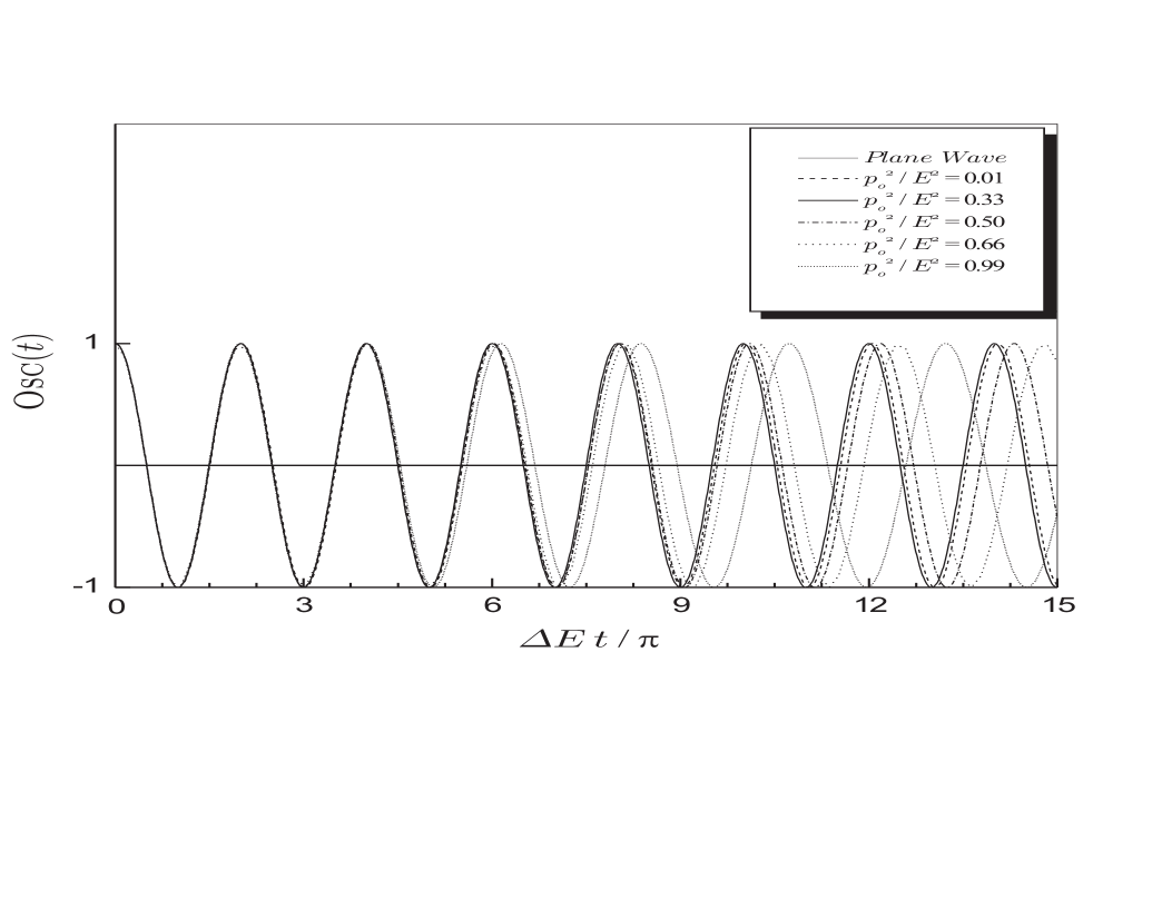
Figure 1: The time-behavior of $\mbox{\sc Osc}(t)$ compared with the standard plane-wave oscillation given by $\cos{[\Delta E\,t]}$ for different propagation regimes. The additional phase $\Theta(t)$ changes the oscillating character after some time of propagation. The minimal deviation occurs for $\frac{p_{\mbox{\tiny$0$}}^{\mbox{\tiny$2$}}}{\bar{E}^{\mbox{\tiny$2$}}}\approx\frac{1}{3}$ which is represented by a solid line superposing the plane-wave case. We have used $a\,\bar{E}=10$ for this plot which was taken from reference Ber05 .

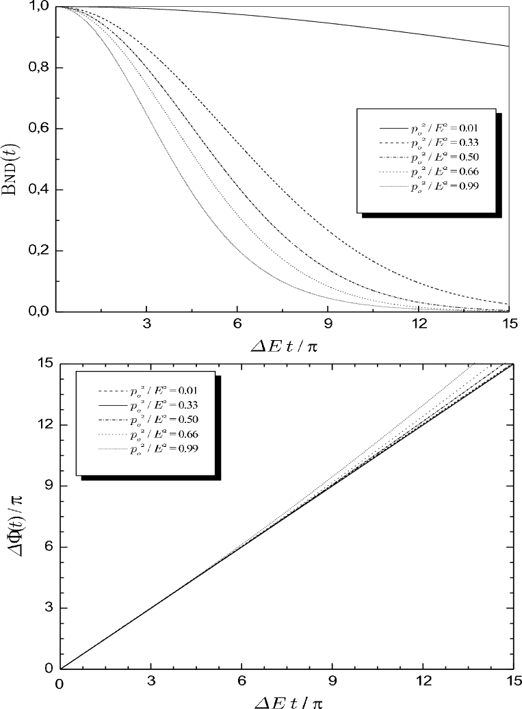
Figure 2: We plot the behavior of the corrected phase $\Delta\Phi(t)=\Delta E\,t+\Theta(t)$ for different propagation regimes and we observe that the values assumed by $\Theta(t)$ are effective only when the interference boundary function $\mbox{\sc Bnd}(t)$ does not vanish. By diminishing the value of the wave packet parameter $a\,\bar{E}$ (we also have used $a\,\bar{E}=10$ for this plot) the amortizing behavior is attenuated and the range of modifications introduced by the additional phase $\Theta(t)$ increases. This plot was taken from reference Ber05 .

The oscillating function $\mbox{\sc Osc}(t)$ of the interference term $\mbox{\sc Int}(t)$ differs from the standard oscillating term, $\cos{[\Delta E\,t]}$, by the presence of the additional phase $\Theta(t)$ which is essentially a second-order correction. The modifications introduced by the additional phase $\Theta(t)$ are discussed in Fig. 1 where we have compared the time-behavior of $\mbox{\sc Osc}(t)$ with $\cos{[\Delta E\,t]}$ for different propagation regimes. The effective bound value assumed by $\Theta(t)$ is determined by the vanishing behavior of $\mbox{\sc Bnd}(t)$. To illustrate this flavor oscillation behavior, we plot both the curves representing $\mbox{\sc Bnd}(t)$ and $\Theta(t)$ in Fig. 2. (both figures are obtained from Ber05 ). We note the phase slowly changing in the NR regime. The modulus of the phase $|\Theta(t)|$ rapidly reaches its upper limit when $\frac{p_{\mbox{\tiny$0$}}^{\mbox{\tiny$2$}}}{\bar{E}^{\mbox{\tiny$2$}}}>\frac{1}{3}$ and, after a certain time, it continues to evolve approximately linearly in time. Essentially, the oscillations vanishes rapidly. By superposing the effects of $\mbox{\sc Bnd}(t)$ in Fig. 2 and the oscillating character $\mbox{\sc Osc}(t)$ expressed in Fig. 1, we immediately obtain the flavor oscillation probability which is explicitly given by

$$P(\mbox{\boldmath$\nu_{\alpha}$}\rightarrow\mbox{\boldmath$\nu_{\beta}$};t)\approx\frac{\sin^{\mbox{\tiny$2$}}{(2\theta)}}{2}\left\{1-\left[1+\mbox{\sc Sp}^{\mbox{\tiny$2$}}(t)\right]^{-\frac{1}{4}}\exp{\left[-\frac{(\Delta\mbox{v}\,t)^{\mbox{\tiny$2$}}}{2a^{\mbox{\tiny$2$}}\left[1+\mbox{\sc Sp}^{\mbox{\tiny$2$}}(t)\right]}\right]}\cos{\left[\Delta E\,t+\Theta(t)\right]}\right\}$$ (19)

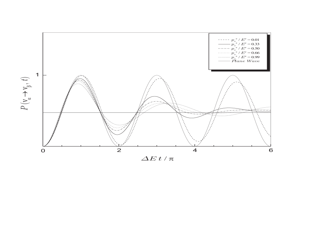
Figure 3: The time-dependence of the flavor conversion probability obtained with the introduction of second-order corrections in the series expansion of the energy for a strictly peaked momentum distribution ($\mathcal{O}(\sigma_{\mbox{\tiny$i$}}^{\mbox{\tiny$3$}})$). By comparing with the PW predictions, depending on the propagation regime, the additional time-dependent phase $\Delta\Phi(t)\equiv\,\Delta E\,t+\Theta(t)$ produces a delay/advance in the local maxima of flavor detection. Phenomenologically, we shall demonstrate that such modifications allow us to quantify small corrections to the averaged values of neutrino oscillation parameters, i. e. the mixing-angle and the mass-squared difference. Essentially, it depends on the product of the wave packet width $a$ by the averaged energy $\bar{E}$. Here again we have used $a\bar{E}=10$.

and illustrated in Fig. 3. Obviously, the larger is the value of $a\,\bar{E}$, the smaller are the wave packet effects.

III Understanding two-flavor oscillation parameters and limits

As earlier extensively discussed in the literature Beu03 ; Kay81 ; Ric93 ; Giu98 , there are various restrictive conditions under which the two-neutrino mixing approximation is valid and the standard PW as well as several classes of WP treatment can be utilized for describing the flavor conversion phenomena. Respecting such limitations, in the previous section we have quantified the second-order corrections introduced by an intermediate WP analysis. Now, we are in position to verify how such modifications can affect the reading of the neutrino oscillation parameter ranges excluded by the confront with experimental data. Therefore, our effective purpose is contrasting the standard PW treatment with the WP analytic study presented in the previous section by re-obtaining the two-flavor neutrino oscillation parameters and limits in a very particular phenomenological context.

From a practical point of view, we have to establish the input experimental parameters as being the detection distance $L_{\mbox{\tiny$0$}}$ (from source), the neutrino energy distribution $\bar{E}$ and the appearance (disappearance) probability $\langle P\rangle$. In addition, to make clear the initial proposition, it is instructive to redefine some parameters which shall carry the main physical information in the oscillation formula, i. e.

$$b_{\mbox{\tiny$0$}}=\frac{1}{2\upsilon}\frac{L_{\mbox{\tiny$0$}}}{E_{\mbox{\tiny$1$}}+{E_{\mbox{\tiny$2$}}}},~{}~{}~{}~{}\delta_{b}=\frac{b_{\mbox{\tiny$0$}}}{a\,\bar{E}}~{}~{}~{}~{}\mbox{and}~{}~{}~{}~{}\upsilon=\frac{p_{\mbox{\tiny$0$}}}{\bar{E}},$$ (20)

with $\bar{E}$ previously defined. For real experiments, $\bar{E}$ and $L_{\mbox{\tiny$0$}}$ can have some spread due to various effects, but in a subset of these experiments, there is a well-defined value of $b_{\mbox{\tiny$0$}}$ about which the events distribute Gro04 . Following the same approach we have adopted while we were analyzing the parameter $\rho$ in Eq. (15), if $\Delta E\ll\bar{E}$, which is perfectly acceptable from the experimental point of view, we can write $\bar{E}=\sqrt{E_{\mbox{\tiny$1$}}{E_{\mbox{\tiny$2$}}}}\approx\frac{1}{2}(E_{\mbox{\tiny$1$}}+{E_{\mbox{\tiny$2$}}})$ so that an effective PW flavor conversion formula can be obtained from Eq. (1) as

$$\langle P\rangle_{\mbox{\tiny PW}}\equiv P(\mbox{\boldmath$\nu_{\alpha}$}\rightarrow\mbox{\boldmath$\nu_{\beta}$};b_{\mbox{\tiny$0$}})=\frac{\sin^{\mbox{\tiny$2$}}{(2\theta)}}{2}\left\{1-\cos{[2\,b_{\mbox{\tiny$0$}}\,\Delta m^{\mbox{\tiny$2$}}]}\right\}.$$ (21)

where $b_{\mbox{\tiny$0$}}$ carries the dependence on the detection distance $L_{\mbox{\tiny$0$}}$ and on the propagation regime ($\upsilon$). Performing some analogous substitutions, the interference terms of Eq. (12) which explicitly appears in the WP flavor conversion formula of Eq. (19) can be read in terms of the above rewritten parameters

$$\mbox{\sc Bnd}(b_{\mbox{\tiny$0$}}) = \left[1+\mbox{\sc Sp}^{\mbox{\tiny$2$}}(b_{\mbox{\tiny$0$}})\right]^{\mbox{\tiny$-$}\frac{1}{4}}\exp{\left[-\frac{2\delta_{b}^{\mbox{\tiny$2$}}\,\upsilon^{\mbox{\tiny$2$}}\,(\Delta m^{\mbox{\tiny$2$}})^{\mbox{\tiny$2$}}}{1+\mbox{\sc Sp}^{\mbox{\tiny$2$}}(b_{\mbox{\tiny$0$}})}\right]},~{}~{}~{}$$ (22)

and

$$\mbox{\sc Osc}(b_{\mbox{\tiny$0$}}) = \cos{\left[2\,b_{\mbox{\tiny$0$}}\,\Delta m^{\mbox{\tiny$2$}}+\Theta(b_{\mbox{\tiny$0$}})\right]},$$ (23)

where

$$\mbox{\sc Sp}(b_{\mbox{\tiny$0$}})=-\rho\frac{\delta_{b}^{\mbox{\tiny$2$}}}{b_{\mbox{\tiny$0$}}}\,\Delta m^{\mbox{\tiny$2$}}$$ (24)

and

$$\Theta(b_{\mbox{\tiny$0$}})=\left[\frac{1}{2}\arctan{\left[\mbox{\sc Sp}(b_{\mbox{\tiny$0$}})\right]}-\frac{b_{\mbox{\tiny$0$}}^{\mbox{\tiny$2$}}\,\upsilon^{\mbox{\tiny$2$}}}{2\delta_{b}^{\mbox{\tiny$2$}}\,\rho^{\mbox{\tiny$2$}}}\frac{\mbox{\sc Sp}^{\mbox{\tiny$3$}}(b_{\mbox{\tiny$0$}})}{\left[1+\mbox{\sc Sp}^{\mbox{\tiny$2$}}(b_{\mbox{\tiny$0$}})\right]}\right],$$ (25)

with $\rho\approx 1-3\upsilon^{\mbox{\tiny$2$}}$. Attempting to the rate $\sigma=\delta_{b}/b_{\mbox{\tiny$0$}}=(a\,\bar{E})^{\mbox{\tiny$-$}1}$ which carries the relevant information concerning with the wave packet width and the averaged energy flux, if it is was sufficiently small ($\sigma\ll 1$) so that we could ignore the second-order corrections of Eq. (9), the probability only with the leading terms could be read as

$$\langle P\rangle_{\mbox{\tiny WP1}}=\frac{\sin^{\mbox{\tiny$2$}}{(2\theta)}}{2}\left\{1-\cos{[2b_{\mbox{\tiny$0$}}\,\Delta m^{\mbox{\tiny$2$}}]}\,\exp{\left[-2(\delta_{b}\,\upsilon\,\Delta m^{\mbox{\tiny$2$}})^{\mbox{\tiny$2$}}\right]}\right\},$$ (26)

which brings up the idea of a coherence length $L_{coh}\sim\frac{a\bar{E}^{\mbox{\tiny$2$}}}{\Delta m^{\mbox{\tiny$2$}}_{\mbox{\tiny$i$}\mbox{\tiny$j$}}}$ Beu03 ; Kie96 and, in the particular case of an UR propagation ($\upsilon=1$), is taken as a reference in the confront with experimental data Gro04 . By the way, despite the relevant dependence on the propagation regime ($\upsilon$), once we are interested in some realistic physical situations, the following analysis will be limited to the UR propagation regime corresponding to the effective neutrino energy of the current flavor oscillation experiments.

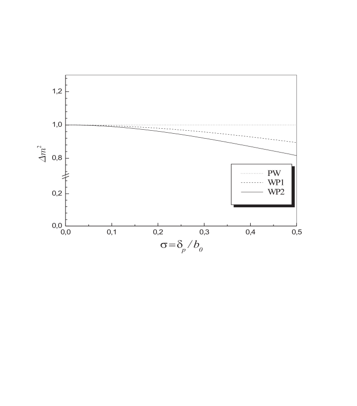
Figure 4: Neutrino oscillation parameter ranges excluded by two experiments: the Palo Verde reactor disappearance experiment (BOEHM 01) and the positive signal from the KamLAND collaboration (EGUCHI 03). We process the input parameters by following the WP treatment with first and second-order corrections (WP1 and WP2) where we have assumed the wave packet parameter $\sigma\sim 0.342$ which leads to a $10\%$ correction to the value of $\Delta m^{\mbox{\tiny$2$}}$ obtained with the PW approximation. In order to compare the results obtained with the WP approach with the PW prediction for the maximum excursion of the curve to the left, which corresponds to an important phenomenological boundary region, we have plotted the PW curve (dotted line) only for the smaller values of $\Delta m^{\mbox{\tiny$2$}}$ (since it has to be averaged on the energy for larger values). The parameter ranges simultaneously allowed by both experiments are represented by the not filled area. The second-order corrections introduce accurate modifications to the oscillation parameter ranges. The nearer is $\sigma$ to 1, the more relevant is the contribution due to higher order terms in the Eq. (10) for determining such accurate limits.

Strictly speaking, most results in the neutrino mixing listings are presented as $\Delta m^{\mbox{\tiny$2$}}$ limits (or ranges) for $\sin^{\mbox{\tiny$2$}}(2\theta)=1$ , and $\sin^{\mbox{\tiny$2$}}(2\theta)$ limits (or ranges) for large $\Delta m^{\mbox{\tiny$2$}}$. Together, they summarize the most of the information contained in the usual $\Delta m^{\mbox{\tiny$2$}}\times\sin^{\mbox{\tiny$2$}}(2\theta)$ plots which provide the parameter exclusion region boundary in the experiments’ papers. Thus, we can compare the PW and WP resolutions by enumerating some relevant aspects which can be observed from the curve $\Delta m^{\mbox{\tiny$2$}}\times\sin^{\mbox{\tiny$2$}}{(2\theta)}$ in the Fig. 4 where the Palo Verde Boe01 and the KamLAND Egu03 experiments/exclusion curves are represented. For the moment, we are interested in the analytical characteristics of such exclusion curves, which, however, we turn to analyze under the phenomenological point of view in section IV. The main aspects to be quantified are:

1) In both PW and WP cases, for large $\Delta m^{\mbox{\tiny$2$}}$ the fast oscillations are completely washed out respectively by the plane-wave resolution or by the smearing out behavior due to the mass-eigenstate wave packet decoherence. Consequently $\sin^{\mbox{\tiny$2$}}{(2\theta)}=2\langle P\rangle$ in this limit.

2) For PW calculations the maximum excursion of the curve to the left occurs at $\Delta m^{\mbox{\tiny$2$}}=\pi/2b_{\mbox{\tiny$0$}}$ when $\sin^{\mbox{\tiny$2$}}{(2\theta)}=\langle P\rangle$. When the WP Eq. (26) is used such a maximal point occurs at the solution of the transcendental equation $-2\sigma^{\mbox{\tiny$2$}}\,\Delta m^{\mbox{\tiny$2$}}\,b_{\mbox{\tiny$0$}}=\tan{[2\,\Delta m^{\mbox{\tiny$2$}}\,b_{\mbox{\tiny$0$}}]}$ which can be approximately given by $\Delta m^{\mbox{\tiny$2$}}\approx\pi/2\,b_{\mbox{\tiny$0$}}\left(1+\mathcal{O}(\sigma^{\mbox{\tiny$2$}})\right)$, but we know that the second-order terms ($\sigma^{\mbox{\tiny$2$}}$) are not being considered. If we had taken into account the second-order corrections in the WP analysis, the maximal value would have been accurately given by $\Delta m^{\mbox{\tiny$2$}}\approx\pi/2\,b_{\mbox{\tiny$0$}}\left(1+2\sigma^{\mbox{\tiny$2$}}+\mathcal{O}(\sigma^{\mbox{\tiny$4$}})\right)$, consequently, a little smaller value than the PW solution.

3) By qualitatively assuming the well-established phenomenological constraints which set $\Delta m^{\mbox{\tiny$2$}}\ll 1\,eV^{\mbox{\tiny$2$}}$ when $\sin^{\mbox{\tiny$2$}}(2\theta)\approx 1$, we can reconstruct the nearly straight-line segment at the bottom of the curve by expanding the probability expressions up to order $\mathcal{O}((\Delta m^{\mbox{\tiny$2$}})^{\mbox{\tiny$2$}})$ so that we can obtain the generic solution

$$\Delta m^{\mbox{\tiny$2$}}\approx\frac{\sqrt{\langle P\rangle_{\mbox{\tiny App}}}}{b_{\mbox{\tiny$0$}}\,\sin{(2\theta)}\,\sqrt{F_{\mbox{\tiny App}}(\sigma)}}$$ (27)

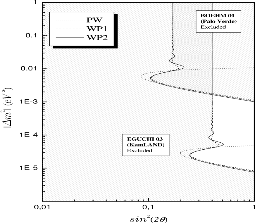
Figure 5: Relative corrections to the $\Delta m^{\mbox{\tiny$2$}}$ value (obtained with the PW analysis) by assuming the WP treatments with first (WP1) and second-order (WP2) corrections in the energy expansion. We normalize the result by dividing $\Delta m^{\mbox{\tiny$2$}}$ by $\frac{\sqrt{\langle P\rangle}}{b_{\mbox{\tiny$0$}}\,\sin{(2\theta)}}$ where obviously $\langle P\rangle_{\mbox{\tiny PW}}=\langle P\rangle_{\mbox{\tiny WP1}}=\langle P\rangle_{\mbox{\tiny WP2}}=\langle P\rangle$ is obtained from the experimental results. For instance, by following the WP treatment with second-order corrections, the correction to the phenomenological parameter $\Delta m^{\mbox{\tiny$2$}}$ corresponds to a diminution of approximately $10\%$ of the $\Delta m^{\mbox{\tiny$2$}}$ PW value when $\sigma\approx 0.342\,(a\bar{E}\approx 3)$, $1\%$ when $\sigma\approx 0.100\,(a\bar{E}\approx 10)$, and $0.1\%$ when $\sigma\approx 0.032\,(a\bar{E}\approx 30)$.

where we have $F_{\mbox{\tiny PW}}(\sigma)=1$ for the PW limit, $F_{\mbox{\tiny WP1}}(\sigma)=1+\sigma^{\mbox{\tiny$2$}}$ for the WP treatment with first-order corrections and $F_{\mbox{\tiny WP2}}(\sigma)=1+2\sigma^{\mbox{\tiny$2$}}+\frac{3}{4}\sigma^{\mbox{\tiny$4$}}$ for the WP treatment with second-order corrections. Eventually, if one had abandoned the analytic calculations and had taken into account higher order terms in the power series expansion of Eq. (10), there would have been some minor corrections to the $\sigma^{\mbox{\tiny$4$}}$ term in $F_{\mbox{\tiny WP2}}$. We discard such minor corrections by assuming $F_{\mbox{\tiny WP2}}(\sigma)\approx 1+2\sigma^{\mbox{\tiny$2$}}$ which, in fact, is the correct approximation when we are considering the energy expansion up to second-order terms and sufficient for comparing the approximations in the Fig. 5. We emphasize that we must consider the second-order term in the series expansion in the Eq. (10) since the modifications emerge with $\sigma^{\mbox{\tiny$2$}}$. As a testing case, we consider the toy model presented in Gro04 where the values of $\sigma=0.23$ and $\sigma=0.3$ are used for plotting the curve $\Delta m^{\mbox{\tiny$2$}}\times\sin^{\mbox{\tiny$2$}}{(2\theta)}$. From an immediate analysis of the Eq. (27) with WP2 approximation we can conclude that more accurate values of $\Delta m^{\mbox{\tiny$2$}}$ are constrict to be diminished by approximately $8\%$ of the value computed with the PW approximation.

Quite generally, the complete analysis of the amortisation coupled to the oscillating character depends upon the experimental features such as the size of the source, which allows us estimating the wave packet width ($a$), the neutrino energy distribution ($\bar{E}$) and the detector resolution ($L_{\mbox{\tiny$0$}}$). Anyway, the main point to be considered is that the characterization of the wave packed ($a$) implicitly described by $\sigma$, which is accompanied by the precise determination of the neutrino energy distribution ($\bar{E}$), plays a fundamental role when the neutrino oscillation parameter and limit accuracy is the subject of the phenomenological analysis. To clarify this point, in addition to the information interpreted from Fig. 5, in the next section we turn back to the phenomenological discussion on the Fig. 4 which illustrates one simple case of parameter determination for reactor neutrinos by considering the results from some disappearance experiments Egu03 ; Boe01 .

IV Phenomenological constraints to reactor experiments - Extension to solar and supernova neutrinos

The first hints that neutrino oscillations actually occur were serendipitously obtained through early studies of solar neutrinos Fuk02 and neutrinos produced in the atmosphere by cosmic rays Fuk00 ; Amb98 . More recently, nuclear reactors and particle accelerators have constituted another source of neutrinos utilized for accurate measurements of flavor oscillation parameters and limits. Reactor neutrino experiments correspond essentially to an electron-antineutrino $\bar{\nu}_{e}$ disappearance experiment where, generically speaking, one looks for the attenuation of the initial neutrino flavor-eigenstate $\nu_{\alpha}$ beam in transit to a detector, where the $\nu_{\alpha}$ is measured. In contrast to the detection of even a few wrong-flavor ($\nu_{\beta}$) neutrinos establishing mixing in an appearance experiment, the disappearance of a few right-flavor ($\nu_{\alpha}$) neutrinos goes unobserved because of statistical fluctuations Gro04 . For this reason, disappearance experiments usually cannot establish small-probabilities ($\sin^{\mbox{\tiny$2$}}{(2\theta)}\ll 1$). Besides, they can fall into several situations Gro04 into which we do not intend to go deep.

By following the purpose of a comparative phenomenological study, we take into account the experimental data from the Palo Verde Boe01 and KamLAND Egu03 experiments by means of which exclusion plots in the plane $\Delta m^{\mbox{\tiny$2$}}\times\sin^{\mbox{\tiny$2$}}{(2\theta)}$ can be elaborated. The Palo Verde experiment Boe01 consists in a disappearance search for $\bar{\nu}_{e}$ oscillations at $0.75-0.89\,km$ distance from the Palo Verde reactors. As consequence of the experimental analysis we assume the input parameter $\langle P\rangle<0.084$ and the averaged energy $\bar{E}$ set in the interval $3.5-4.2\,MeV$. The KamLAND collaboration Egu03 observes reactor $\bar{\nu}_{e}$ disappearance at $\sim 180\,km$ baseline to various Japanese nuclear power reactors. This is the lower limit on the mass difference spread unlike all other disappearance experiments Egu03 and the observation is consistent with neutrino oscillations, with mass-difference and mixing angle parameters in the Large Mixing Angle Solution region of the solar neutrino problem. In this case, we assume the input parameter $\langle P\rangle>0.2$ with the reactor $\bar{\nu}_{e}$ energy spectrum smaller than $8\,MeV$ and an analysis threshold of $2.6\,MeV$ where the experiment sensitive $\Delta m^{\mbox{\tiny$2$}}$ range is set down to $10^{\mbox{\tiny$-$}\mbox{\tiny$5$}}eV^{\mbox{\tiny$2$}}$ Egu03 . The important point we attempt in the Fig. 4 is the comparative modifications due to second-order corrections, i. e. we are not setting extremely accurate input (experimental) parameters but we are setting a more accurate procedure for obtaining the output parameter ($\Delta m^{\mbox{\tiny$2$}}$ and $\theta$) ranges and limits.

The analysis of solar neutrino Fuk02 ; Ahm02 measurements involves considerable input from solar physics and the nuclear physics involved in the extensive chain of reactions that together are termed “Standard Solar Model” (SSM) SSM . Since the predicted flux of solar neutrinos from SSM is very well-established SSM we know that the low energy $p-p$ neutrinos are the most abundant and, since they arise from reactions that are responsible for most of the energy output of the sun, the predicted flux of these neutrinos is constrained very precisely ($\pm 2\%$) by the solar luminosity. The same is not true for higher energy neutrinos for which the flux is less certain due to uncertainties in the nuclear and solar physics required to compute them.

In fact, the true frontier for solar neutrino experiments is the real-time, spectral measurement of the flux of neutrinos below $0.4\,MeV$ produced by $p-p$ reactions. Measurements of the $p-p$ flux to an accuracy comparable to the accuracy of the SSM calculation will significantly improve the precision of the mixing angle Bah03 ; Ban03 . In addition, if the total $p-p$ flux is well-know, measurement of the active component can help constrain a possible sterile admixture Gro04 . Therefore, an accurate phenomenological analysis for obtaining small modifications to the oscillation parameters, as we have illustrated in the Fig. 4, can be really pertinent. In this context, the experimental challenge is to achieve low background at low energy threshold. In particular, a number of projects and proposals aiming to build $p-p$ neutrino spectrometers are discussed in Der04 where it has been shown that a large volume liquid organic scintillator detector with an energy resolution of $10\,keV$ at $200\,keV$ can be sensitive to solar $p-p$ neutrinos, if operated at the target radiopurity levels for the Borexino detector, or the solar neutrino project of KamLAND Egu03 . In spite of the higher energy neutrinos being more accessible experimentally, the corrections to the wave packet formalism can be physically relevant for $p-p$ neutrinos with energy distributed around an averaged value of $\bar{E}\approx 10-100\,keV$. Following some standard procedure Kim93 for calculating the neutrino flux wave packet width $a$ for $p-p$ solar reactions, we obtain $a=10^{\mbox{\tiny$-$}10}-10^{\mbox{\tiny$-$}8}\,m\equiv 0.5-50\,(keV)^{\mbox{\tiny$-$}1}$. Such an interval sets a very particular range for the $\sigma$ parameter comprised by the interval $5\cdot 10^{\mbox{\tiny$-$}\mbox{\tiny$5$}}-0.2$ for $\bar{E}\approx 0.01-0.4\,MeV$ which introduces the possibility for WP second-order corrections establish some not ignoble modifications for the $p-p$ neutrino oscillation parameter limits.

Turning back to the confront between the PW and the WP formalism, once we had precise values for the input parameters $\langle P\rangle$, $L_{\mbox{\tiny$0$}}$ and $\bar{E}$,we could determine the effectiveness of the first/second-order corrections in determining $\Delta m^{2}$ for any class of neutrino oscillation experiment. For instance, the flux of atmospheric neutrinos produced by collisions of cosmic rays (which are mostly protons) with the upper atmosphere is measured by experiments prepared for observing $\nu_{e}\leftrightarrow\nu_{\mu}$ and $\bar{\nu}_{e}\leftrightarrow\bar{\nu}_{\mu}$ conversions. In particular, SuperKamiokande Fuk00 and MACRO Amb98 measurements also work on the $\nu_{\mu}\leftrightarrow\nu_{\tau}$ conversion. The neutrino energies range about from $0.1\,GeV$ to $100\,GeV$ which constrains the relevance of WP effects to an wave packet width $a\sim 10^{\mbox{\tiny$-$}\mbox{\tiny$1$}\mbox{\tiny$2$}}\,m$. The accelerators experiments Ana98 ; Agu01 ; Arm02 cover a higher variety of neutrino flavor conversions where the neutrino energy flux stays around $1-10\,GeV$ the limitations to the wave packet width $a$ (see the Table 1) are analogous which makes the WP second-order corrections, as a first analysis, completely irrelevant.

The most prominent contribution from the above discussion in determining the oscillation parameters and limits can come with the analysis of supernova neutrinos which, however, are not yet solidly established by the experimental data. Neutrinos from SN1987A in the Large Magellanic Cloud were detected by Kamiokande and IMB detectors - only 19 events. Nowadays, SuperKamiokande, SNO, LVD, ICARUS, IceCube are expected to detect events from the next galactic supernova and improve the statistics, providing new information on neutrino properties and supernova. The main problem in studying neutrinos oscillation from supernova is the spectral and temporal evolution of the neutrino burst. In a supernova, the size of the wave packet is determined by the region of production (plasma), due to a process known as pressure broadening, which depends on the temperature, the plasma density, the mean free path of the neutrino producing particle and its mean termal velocity Kim93 . Neutrinos from supernova core with $100\,MeV$ energy have a wave packet size varying from $\sim 5\cdot 10^{\mbox{\tiny$-$}\mbox{\tiny$1$}\mbox{\tiny$6$}}\,m$ to $\sim 10^{\mbox{\tiny$-$}\mbox{\tiny$1$}\mbox{\tiny$4$}}\,m$ which leads to a wave packet parameter $a\bar{E}$ comprised by the interval $0.25-5$ for which the second-order corrections can be relevant if $a\bar{E}>1$. There also are $10\,MeV$ neutrinos, from neutrinosphere, with a wave packet size of approximately $10^{\mbox{\tiny$-$}\mbox{\tiny$1$}\mbox{\tiny$2$}}\,m$ with $a\bar{E}\approx 50$.

In table 1 we summarize the results for the five well-known neutrino sources: reactor, solar, atmospheric, accelerator and supernova. We compare the size of the wave packet $a$ determined by the region within which the production process of a neutrino is effectively localized by the physical process itself (for instance, from a cross section analysis) with the limits below which the WP second-order corrections set a more accurate value to the mass-squared difference $\Delta m^{\mbox{\tiny$2$}}$. It allow us to establish where/when the physical effects due to second-order corrections can be eventually be expected.

The limits presented in table 1 represents, for instance, a diminution of $10\%$, $1\%$ and $0.1\%$ from the value computed with the PW approach. However, a pertinent objection to the the representativeness of such values can be stated: it is important to observe that neutrino energy measurements cannot be performed very precisely so that this produces an effect competing with that of the finite size of the wave packet. If we set the energy uncertainty represented by $\delta E$, the Heisenberg uncertainty relation states that $\delta E\,a\sim 1$ and, consequently, our approximation hypothesis leads to $\frac{\delta E}{\bar{E}}\sim\frac{1}{a\,\bar{E}}\ll 1$. Realistically speaking, a typical neutrino-oscillation experiment searches for flavor conversions by means of an apparatus which, apart from the details inherent to the physical process, provides an indirect measurement of the neutrino energy (in each event) accompanied by an experimental error $\Delta E_{exp}$ due to the “detector resolution”. In case of $\frac{\Delta E_{exp}}{\bar{E}}<\frac{\delta E}{\bar{E}}\sim\frac{1}{a\,\bar{E}}$ the effective role of the second-order corrections illustrated in this analysis can be relevant. On the contrary, $\Delta E_{exp}>\delta E$ demands for an averaged energy integration where the decoherence effect through imperfect neutrino energy measurements by far dominates. In a quantitative analytical analysis, this problem could be overcome by performing an analytical energy integration which, in general, is not possible. In the present context, the current experimental values/measurements set some limitations to the applicability of our analysis by restricting it to the ${}^{\mbox{\tiny$7$}}Be$ and $pe^{\mbox{\tiny$-$}}p$ lines for solar neutrinos for which the energy flux is precisely defined ($\frac{\Delta E_{exp}}{\bar{E}}\ll 1$) and, eventually, to some (next generation) reactor experiment and, certainly, to supernova neutrinos.

As an additional remark, without comprehending the exact theoretical coupled to experimental procedure for determining the wave packet widths for a certain type of neutrino flux, we cannot arbitrarily assume, apart from the obvious criticisms to the PW approach, the modifications introduced by the WP treatment (particularly with second-order corrections) are irrelevant in the confront with a generic class of neutrino experimental data. Finally, from the phenomenological point of view, the general arguments presented in Gro04 continue to be valid, i. e. the above discussion has so far been limited to vacuum oscillations, where the mixing probabilities are described in terms of the mixing angle. In the solar neutrino case it is likely that interactions between the neutrinos and solar electrons affect the oscillation probability MSW .

V Conclusion

We have reported about the intermediate WP prescription in the context of neutrino flavor oscillations from which, under the particular assumption of a sharply peaked momentum distribution which sets an analytical approximation of order $\mathcal{O}((a\bar{E})^{\mbox{\tiny$-$}\mbox{\tiny$3$}})$, we have re-obtained an explicit expression for the flavor conversion formula for (U)R and NR propagation regimes. By concentrating our arguments on quantifying the second-order effects of such an approximation, we have observed that the existence of an additional time-dependent phase in the oscillating term of the flavor conversion formula and the modified spreading effect can represent some minor but accurate modifications to the (ultra)relativistic oscillation probability formula which leads to important corrections to the phenomenological analysis for obtaining the neutrino oscillation parameter and limits.

In particular, we have quantified such effects for determining the corrections to the $\Delta m^{\mbox{\tiny$2$}}\times\sin^{\mbox{\tiny$2$}}{(2\theta)}$ curve for two reactor experiments Boe01 ; Egu03 . The oscillation parameter range deviation from the PW values depends effectively on the product between the wave packet width $a$ and the averaged energy flux $\bar{E}$ which characterizes the detection process. The importance of the second-order corrections which come from the WP construction can also be relevant in the framework of three-neutrino mixing. It is well diffused that the next question which can be approached experimentally is that of $e3$ mixing. A consequence of a non-zero $U_{e\mbox{\tiny$3$}}$ matrix element will be a small appearance of $\nu_{e}$ in a bean of $\nu_{\mu}$: for the particular case where $\Delta m^{\mbox{\tiny$2$}}_{\mbox{\tiny$1$}\mbox{\tiny$2$}}\ll\Delta m^{\mbox{\tiny$2$}}_{\mbox{\tiny$2$}\mbox{\tiny$3$}}$ (experimental data), and for $\bar{E}_{\nu}\sim L\,\Delta m^{\mbox{\tiny$2$}}_{\mbox{\tiny$2$}\mbox{\tiny$3$}}$, ignoring matter effects, we can find Kim93

$$P(\mbox{\boldmath$\nu_{\mu}$}\rightarrow\mbox{\boldmath$\nu_{e}$};L)=\sin^{\mbox{\tiny$2$}}{(2\theta{\mbox{\tiny$1$}\mbox{\tiny$3$}})}\,\sin^{\mbox{\tiny$2$}}{(\theta{\mbox{\tiny$2$}\mbox{\tiny$3$}})}\sin^{\mbox{\tiny$2$}}{\left[\frac{\Delta m^{\mbox{\tiny$2$}}_{\mbox{\tiny$2$}\mbox{\tiny$3$}}\,L}{4\bar{E}}\right]}.$$ (28)

This expression illustrates that $\theta_{\mbox{\tiny$1$}\mbox{\tiny$3$}}$ manifests itself in the amplitude of an oscillation with 2-3 like parameters. By assuming an intermediate wave packet analysis, fine-tuning corrections can eventually be relevant.

Experimentally, since the modulation may be parts per thousand or smaller, one needs both good statistics and low background data. For instance the KamLAND experiment will significantly reduce the allowed region for $\Delta m^{\mbox{\tiny$2$}}_{\mbox{\tiny$1$}\mbox{\tiny$2$}}$ and $\sin{(2\theta_{\mbox{\tiny$1$}\mbox{\tiny$2$}})}$ relative to the present results, where the second-order wave packet corrections can appear as an additional ingredient for accurately applying the phenomenological analysis. At the same time, the next major goal for the reactor neutrino program will be to attempt a measurement of $\sin^{\mbox{\tiny$2$}}{(2\theta_{\mbox{\tiny$1$}\mbox{\tiny$3$}})}$. It can be shown that the reactor experiments have the potential to determine $\theta_{\mbox{\tiny$1$}\mbox{\tiny$3$}}$ without ambiguity from CP violation or matter effects (by assuming the necessary statistical precision which requires large reactor power and large detector size). With reasonable systematic errors ($<\,1\%$) the sensitivity is supposed to reach about $\sin^{\mbox{\tiny$2$}}{(2\theta_{\mbox{\tiny$1$}\mbox{\tiny$3$}})}\approx 0.01-0.02$ Vog04 and an accurate method of analysis, maybe in the wave packet framework, can be required.

Turning back to the foundations for applying the intermediate wave packet formalism in the neutrino oscillation problem, we know the necessity of a more sophisticated approach is required. It can involve a field-theoretical treatment. Derivations of the oscillation formula resorting to field-theoretical methods are not very popular. They are thought to be very complicated and the existing quantum field computations of the oscillation formula do not agree in all respects Beu03 . The Blasone and Vitiello (BV) model Bla95 ; Bla03 to neutrino/particle mixing and oscillations seems to be the most distinguished trying to this aim. They have attempt to define a Fock space of weak eigenstates to derive a nonperturbative oscillation formula. Also with Dirac wave packets, the flavor conversion formula can be reproduced Ber04B with the same mathematical structure as those obtained in the BV model Bla95 ; Bla03 . In fact, both frameworks deserve a more careful investigation since the numerous conceptual difficulties hidden in the quantum oscillation phenomena still represent an intriguing challenge for physicists.

Table 1: Wave packet width $a$ estimative for which the WP second-order corrections start to be relevant in obtaining an accurate value of $\Delta m^{\mbox{\tiny$2$}}$. We have computed the $a$ limit by assuming $10\%(\sigma\sim 0.342)$, $1\%(\sigma\sim 0.100)$ and $0.1\%(\sigma\sim 0.032)$, corrections to the value computed with the PW approximation.

$\nu$ class	Process(Abbr.)	Ref.	$\bar{E}(MeV)$	$a_{\mbox{\tiny$1$}}(10^{\mbox{\tiny$-$}\mbox{\tiny$1$}\mbox{\tiny$2$}}m)$	$a_{\mbox{\tiny$2$}}(10^{\mbox{\tiny$-$}\mbox{\tiny$1$}\mbox{\tiny$2$}}m)$	$a_{\mbox{\tiny$3$}}(10^{\mbox{\tiny$-$}\mbox{\tiny$1$}\mbox{\tiny$2$}}m)$	$a_{\mbox{\tiny Theo.}}(m)$
				($10\%$ )	($1\%$)	($0.1\%$)	Ref.Kim93
Reactor	$\nu_{e}\rightarrow\backslash\hskip 9.95863pt\nu_{e}$	Egu03 , Boe01	$\sim 3$	$\sim 0.2$	$\sim 0.7$	$\sim 2.1$	$\sim 10^{\mbox{\tiny$-$}\mbox{\tiny$6$}}$
	$pp$	SSM	$\sim 0.1$	$\sim 6$	$\sim 20.0$	$\sim 63.2$
	${}^{\mbox{\tiny$7$}}Be$	SSM	$\sim 0.9$	$\sim 1.5$	$\sim 5.0$	$\sim 15.8$
Solar	${}^{\mbox{\tiny$1$}\mbox{\tiny$3$}}N,\,^{\mbox{\tiny$1$}\mbox{\tiny$5$}}O,\,^{\mbox{\tiny$1$}\mbox{\tiny$7$}}F$	SSM	$\sim~{}~{}1$	$\sim 0.6$	$\sim 2.0$	$\sim 6.3$	$\sim 10^{\mbox{\tiny$-$}\mbox{\tiny$9$}}$
($BP2000$)	$pe^{\mbox{\tiny$-$}}p$	SSM	$\sim 1.4$	$\sim 0.4$	$\sim 1.4$	$\sim 4.5$
	${}^{\mbox{\tiny$8$}}B,\,hep$	SSM	$\sim~{}10$	$\sim 0.06$	$\sim 0.2$	$\sim 0.6$
Atmospheric	$\nu_{\mu}\rightarrow\nu_{e,\tau,s}$	Fuk02 ; Amb98	$10^{\mbox{\tiny$2$}\,\mbox{\tiny to}\,\mbox{\tiny$5$}}$	$6\cdot 10^{\mbox{\tiny$-$}\mbox{\tiny$3$}\,\mbox{\tiny to}\,\mbox{\tiny$-$}\mbox{\tiny$6$}}$	$2\cdot 10^{\mbox{\tiny$-$}\mbox{\tiny$2$}\,\mbox{\tiny to}\,\mbox{\tiny$-$}\mbox{\tiny$5$}}$	$6\cdot 10^{\mbox{\tiny$-$}\mbox{\tiny$2$}\,\mbox{\tiny to}\,\mbox{\tiny$-$}\mbox{\tiny$5$}}$	$-$$-$$-$
Accelerator	$\nu_{\mu}(\bar{\nu}_{\mu})\rightarrow\nu_{e}(\bar{\nu}_{e})$	Agu01	$10^{\mbox{\tiny$3$}\,\mbox{\tiny to}\,\mbox{\tiny$4$}}$	$6\cdot 10^{\mbox{\tiny$-$}\mbox{\tiny$4$}\,\mbox{\tiny to}\,\mbox{\tiny$-$}\mbox{\tiny$5$}}$	$2\cdot 10^{\mbox{\tiny$-$}\mbox{\tiny$3$}\,\mbox{\tiny to}\,\mbox{\tiny$-$}\mbox{\tiny$4$}}$	$6\cdot 10^{\mbox{\tiny$-$}\mbox{\tiny$3$}\,\mbox{\tiny to}\,\mbox{\tiny$-$}\mbox{\tiny$4$}}$	$\sim 1$
Supernova	$-$$-$$-$	$-$$-$$-$	$\sim~{}10^{2}$	$\sim 6\cdot 10^{\mbox{\tiny$-$}\mbox{\tiny$3$}}$	$\sim 2\cdot 10^{\mbox{\tiny$-$}\mbox{\tiny$2$}}$	$\sim 6\cdot 10^{\mbox{\tiny$-$}\mbox{\tiny$2$}}$	$\sim 10^{\mbox{\tiny$-$}\mbox{\tiny$1$}5}$
(estimative)