Mixing of scalar tetraquark and quarkonia states in a chiral approach

Francesco Giacosa

Institut für Theoretische Physik
Universität Frankfurt
Johann Wolfgang Goethe - Universität
Max von Laue–Str. 1
60438 Frankfurt, Germany
e-mail: giacosa@th.physik.uni-frankfurt.de

A chiral invariant Lagrangian describing the tetraquark-quarkonia interaction is considered at the leading and subleading order in the large-$N_{c}$ expansion. Spontaneous chiral symmetry breaking generates mixing of scalar tetraquark and quarkonia states and non-vanishing tetraquark condensates. In particular, the mixing strength is related to the decay strengths of tetraquark states into pseudoscalar mesons. The results show that scalar states below 1 GeV are mainly four-quark states and the scalars between 1 and 2 GeV quark-antiquark states, probably mixed with the scalar glueball in the isoscalar sector.

1 Introduction

The spectroscopic interpretation of the scalar states below 1 GeV represents an important issue of modern hadronic physics. It is not yet clear if the dominant contribution to their wave function constitutes of quarkonia, mesonic molecules or Jaffe’s tetraquark states. In turn, this subject is strongly connected to the nature of the scalar states above 1 GeV (we refer to the review papers [1, 2, 3]).

Various interpretations have been proposed in the literature about the scalar resonances below and above 1 GeV. According to the most popular scenario, one interprets the isovector and isotriplet resonances $a_{0}(1450)$ and $K(1430)$ as the ground-state quark-antiquark bound states. The three isoscalar resonances $f_{0}(1370)$, $f_{0}(1500)$ and $f_{0}(1710)$ are an admixture of two isoscalar quarkonia and bare glueball configurations (we refer to [1, 2, 4, 5, 6, 7, 8, 9, 10, 11] and Refs. therein; recently the inclusion of hybrids in the mixing scheme has been performed in Ref. [12]). As a consequence, the scalar states below 1 GeV ($f_{0}(600),$ $k(800),$ $f_{0}(980)$ and $a_{0}(980)$) must be something else, like (loosely bound) mesonic molecular states [13, 14], dynamical generated resonances [15] or Jaffe’s tetraquark states [1, 3, 16, 17, 18]. It is indeed possible that an interplay of these three possibilities takes place.

The tetraquark states, whose building blocks are a diquark ($q^{2}$) and an antidiquark ($\overline{q}^{2}$), play a central role in this paper. Calculations based on one-gluon exchange [1, 19], instantons [20, 21], Nambu Jona–Lasinio model (NJL) [22] and Dyson-Schwinger equation (DSE) [23] support a strong attraction among two quarks in a color antitriplet ($\overline{3}_{C}$), a flavor antitriplet ($\overline{3}_{F}$) and spinless configuration [1, 16] (color and flavor triplets are realized for an antidiquark). Naively speaking, such a scalar diquark ‘behaves like an antiquark’ from a flavor (and color) point of view, thus a nonet of light scalar tetraquark states naturally emerges in this context. Support for the existence of Jaffe’s states below 1 GeV is in agreement with the Lattice studies of Refs. [24, 25, 26].

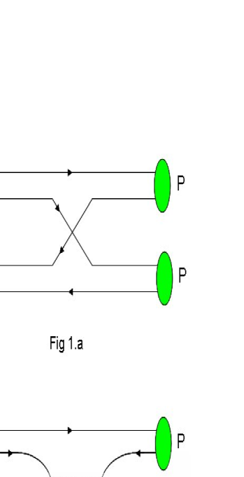
Figure 1: Dominant (1.a) and subdominant (1.b) contributions to the transition amplitudes of a scalar tetraquark state into two pseudoscalar mesons. They correspond to the Lagrangian in Eqs. (21)-(22).

In the recent work of Ref. [18] the present author analyzed the strong and the electromagnetic decays of the light scalar states $\{f_{0}(600),$ $k(800),$ $f_{0}(980)$ and $a_{0}(980)\}$ interpreted as Jaffe’s tetraquark states, which naturally account for the mass degeneracy of $f_{0}(980)$ and $a_{0}(980)$ and their large $\overline{K}K$ decay strength. The dominant (Fig. 1.a) and the subdominant (Fig. 1.b) decay mechanisms in the large-$N_{c}$ expansion, respectively proportional to the decay strengths $c_{1}$ and $c_{2}$, have been systematically taken into account in an effective $SU_{V}(3)$-invariant interaction Lagrangian.

In the present work we extend the model of Ref. [18], which was built under the requirement of flavor symmetry $SU_{V}(3)$, by considering invariance under the chiral group $SU_{R}(3)\times SU_{L}(3)$. The explicit inclusion of a scalar quarkonia nonet, lying between 1 and 2 GeV (see discussion in Section 2.1) as the chiral partner of the pseudoscalar nonet, and the inclusion of the pseudoscalar diquark, as the chiral partner of the scalar diquark, are required. As in [18] we keep the leading and the subleading terms in the large-$N_{c}$ expansion.

As a consequence of chiral symmetry breaking, mixing among tetraquark and quarkonia states takes place. The most important theoretical result of the present work is the possibility to relate the mixing strength between the scalar tetraquark and quarkonia nonets to the tetraquark decay strengths $c_{1}$ and $c_{2}$ of Fig. 1 and to the pion and kaon decay constants. Furthermore, the tetraquark-quarkonia mixing in the scalar sector is responsible for the emergence of non-vanishing tetraquark condensates.

The connection of the decay strengths $c_{1}$ and $c_{2}$ to the mixing allows us to evaluate its strength. As a result we find that the tetraquark assignment for the light scalar states is consistent: by analyzing the isovector channel the resonance $a_{0}(980)$ has a dominant tetraquark content; the quarkonium amount in its spectroscopic wave function turns out to be relatively small ($\lesssim 10\%$). An analogous result is obtained in the kaonic sector.

The use of chiral Lagrangian for the analysis of tetraquark-quarkonia mixing has been studied in Refs. [33, 34, 35, 36], where sizable admixtures in the scalar physical resonances below and above 1 GeV are found. In the present work a different chiral Lagrangian is utilized and only the scalar (and not the pseudoscalar) diquarks are considered as basic constituent for low-energy mesonic resonances. Our results point to a smaller mixing strength and thus to a substantial separation of four-quark states below 1 GeV and quarkonia states above 1 GeV.

The paper is organized as follows. In Section 2 the model is constructed: we recall the basics of the chiral treatment of the scalar and pseudoscalar nonets, we introduce the scalar diquark and briefly review Ref. [18], we describe the pseudoscalar diquark and write down the chiral invariant tetraquark-quarkonia interaction Lagrangian. In section 3 the phenomenological implications are studied: the scalar tetraquark-quarkonia mixing and the magnitude of the tetraquark condensates. In section 4 we present the summary and the conclusions.

2 Set-up of the model

2.1 Quarkonia nonets

We briefly recall the basic elements for the set up of the pseudoscalar and the scalar quarkonia nonets. At a microscopic level one has the quark field $q_{i}(x)$ with $i=u,d,s.$ The right and left spinors are given by:

$$q_{i,R} = P_{R}q_{i},\text{ }q_{i,R}^{{\dagger}}=q_{i}P_{R},\text{ }\overline{q}_{i,R}=\overline{q}_{i}P_{L}$$ (1)

$$\text{ }q_{i,L} = P_{L}q_{i},\text{ }q_{i,L}^{{\dagger}}=q_{i}P_{L},\text{ }\overline{q}_{i,L}=\overline{q}_{i}P_{R},$$ (2)

where $P_{R}=\frac{1}{2}\left(1+\gamma_{5}\right)$ and $P_{L}=\frac{1}{2}\left(1-\gamma_{5}\right).$

The $SU_{R}(3)\times$ $SU_{L}(3)$ transformation on the quark fields is defined as:

$$q_{i}=q_{i,R}+q_{i,L}\rightarrow R_{ij}q_{j,R}+L_{ij}q_{j,L}\text{ with: }R\in SU_{R}(3)\text{, }L\in SU_{L}(3).$$ (3)

Out of quark fields one can build up operators (currents) with the correct quantum numbers of the physical resonances. In fact, at a composite level one deals with mesons, which have the same transformation properties of the underlying quark currents. In Table 1 we summarize the properties of the pseudoscalar and scalar quarkonia Hermitian matrices $\mathcal{P}$ and $\mathcal{S}$ and of the matrix $\Sigma=\mathcal{S}+i\mathcal{P}$: the corresponding matrix elements and the components in the Gell-Mann basis (denoted as ‘currents’ in Table 1), the transformations under parity (P), charge conjugation (C), $SU_{V}(3)$ (occurring for $R=L=U$ in Eq. (3)), chiral $SU_{R}(3)\times$ $SU_{L}(3)$ and $U_{A}(1)$ (occurring for $q_{i}\rightarrow e^{i\nu\gamma_{5}}q_{i},$ i.e. $q_{i,R}\rightarrow e^{i\nu}q_{i,R}$ and $q_{i,L}\rightarrow e^{-i\nu}q_{i,L}$) are reported.

Table 1: Summary of the properties of $\mathcal{P},$ $\mathcal{S}$ and $\Sigma$.

	$\mathcal{P}=\frac{1}{\sqrt{2}}\sum_{i=0}^{8}P^{i}\lambda_{i}$	$\mathcal{S=}\frac{1}{\sqrt{2}}\sum_{i=0}^{8}S^{i}\lambda_{i}$	$\Sigma=\mathcal{S}+i\mathcal{P}$
Matrix Elements	$\mathcal{P}_{ij}\equiv\overline{q}_{j}i\gamma^{5}q_{i}$	$\mathcal{S}_{ij}\equiv\overline{q}_{j}q_{i}$	$\Sigma_{ij}\equiv 2\overline{q}_{j,R}q_{i,L}$
Currents	$P^{i}\equiv\overline{q}i\gamma^{5}\frac{\lambda_{i}}{\sqrt{2}}q$	$S^{i}\equiv\overline{q}\frac{\lambda_{i}}{\sqrt{2}}q$	$\Sigma^{i}\equiv 2\overline{q}_{R}\frac{\lambda_{i}}{\sqrt{2}}q_{L}$
P	$-\mathcal{P(}x^{0},-\mathbf{x}\mathcal{)}$	$\mathcal{S(}x^{0},-\mathbf{x}\mathcal{)}$	$\Sigma^{\dagger}\mathcal{(}x^{0},-\mathbf{x}\mathcal{)}$
C	$\mathcal{P}^{t}$	$\mathcal{S}^{t}$	$\Sigma^{t}$
$SU_{V}(3)$	$U\mathcal{P}U^{\dagger}$	$U\mathcal{S}U^{\dagger}$	$U\Sigma U^{\dagger}$
$SU_{R}(3)\times$ $SU_{L}(3)$	$\frac{1}{2i}\left(L\Sigma R^{\dagger}-R\Sigma^{\dagger}L^{\dagger}\right)$	$\frac{1}{2}\left(L\Sigma R^{\dagger}+R\Sigma^{\dagger}L^{\dagger}\right)$	$L\Sigma R^{\dagger}$
$U_{A}(1)$ ($q_{i}\rightarrow e^{i\nu\gamma_{5}}q_{i}$)	$\frac{1}{2i}\left(e^{-2i\nu}\Sigma-e^{2i\nu}\Sigma^{\dagger}\right)$	$\frac{1}{2}\left(e^{-2i\nu}\Sigma+e^{2i\nu}\Sigma^{\dagger}\right)$	$e^{-2i\nu}\Sigma$

Following [30] and Refs. therein, which we refer to for a careful treatment, we introduce the Lagrangian $\mathcal{L}_{\Sigma}$

$$\mathcal{L}_{\Sigma}=\frac{1}{4}Tr\left[\partial_{\mu}\Sigma\partial^{\mu}\Sigma^{{\dagger}}\right]-V_{0}(\Sigma,\Sigma^{{\dagger}})-V_{SB}(\Sigma,\Sigma^{{\dagger}})$$ (4)

($Tr$ denotes trace over flavor) which describes the dynamics of the pseudoscalar and scalar quarkonia mesons. As usual, $V_{0}$ represents the chiral invariant potential while $V_{SB}$ encodes symmetry breaking due to the non-zero current quark masses. In the present work we are not concerned with the detailed description of the properties of the potentials $V_{0}$ and $V_{SB}$. What is important for us is spontaneous chiral symmetry breaking ($\chi SB$), that is the minimum of the potential $V_{0}+V_{SB}$ is realized for non-zero vacuum expectation values ($vev$’s):

$$\left\langle\mathcal{S}_{ij}\right\rangle=\alpha_{i}\delta_{ij}\text{ (with }\alpha_{u}=\alpha_{d}\text{: isospin symmetry).}$$ (5)

The expectation values $\alpha_{i}$ are related to the pion and the kaon decay constants in a model independent way [30, 37]:

$$\left\langle\mathcal{S}_{11}\right\rangle+\left\langle\mathcal{S}_{22}\right\rangle=2\alpha_{u}=\sqrt{2}F_{\pi}\text{, }\left\langle\mathcal{S}_{11}\right\rangle+\left\langle\mathcal{S}_{33}\right\rangle=\alpha_{u}+\alpha_{s}=\sqrt{2}F_{K}\text{.}$$ (6)

We use $F_{\pi}=0.0924$ GeV and $F_{K}=1.22F_{\pi}$. This leads us to shift the matrix $\Sigma$ as:

$$\Sigma=\mathcal{S}+i\mathcal{P\rightarrow}\Sigma=\Sigma_{0}+\mathcal{S}+i\mathcal{P}\text{ where: }\Sigma_{0}=diag\{\alpha_{u},\alpha_{u},\alpha_{s}\}.$$ (7)

The pseudoscalar nonet is well established: $\mathcal{P\equiv}\{\pi,K,\eta,\eta^{\prime}\}.$ The identification of the scalar states is controversial. Some models [22, 38, 39, 40] identify the resonance $f_{0}(600)$ as the chiral partner of the pion, hence a quarkonium $\overline{n}n=\sqrt{1/2}(\overline{u}u+\overline{d}d)$. This assignment encounters a series of well-known problems: (i) in this scheme the resonances $a_{0}^{0}(980)$ and $f_{0}(980)$ would be respectively $\sqrt{1/2}(\overline{u}u-\overline{d}d)$ and $\overline{s}s.$ Their mass degeneracy is then hard to be explained from their quark content (see also the different point of view in Refs. [39, 40]) (ii) The strong coupling of $a_{0}(980)$ to $\overline{K}K$ cannot be explained within this assignment (the points (i)-(ii) are naturally explained when interpreting the light scalar resonance as mainly Jaffe’s four-quark states, see Refs. [16, 3, 17, 18] and next subsection). (iii) The scalar quarkonia states are p-wave $(L=S=1),$ therefore expected to have a mass comparable to the p-wave nonets of tensor and axial-vector mesons which lie well above 1 GeV. (iv) The Lattice results of Refs. [26, 41] predict a mass for the quarkonium state $u\overline{d}$ about $1.4$-$1.5$ GeV, thus well above 1 GeV (see also the different result of Ref. [42]). (v) As shown in Ref. [43] (and recently confirmed in Ref. [44] at two-loop order in unitarized Chiral Perturbation Theory for the resonance $f_{0}(600)$) the large-$N_{c}$ behavior of the masses of the scalar states below 1 GeV is $not$ compatible with a dominant quarkonium content, thus further pointing to a heavier bare mass of the latter.

Thus, we expect that the bare quarkonia masses lie above 1 GeV. We will then analyze the mixing of the quarkonia states with the (lighter) four-quark states in Section 3.

2.2 Scalar diquark and corresponding tetraquark states

We turn our attention to the scalar diquark current. To this end we consider the following scalar flavour-antisymmetric ($\overline{3}_{F}$) diquark-matrix $D$:

$$D_{ij}\equiv\sqrt{\frac{1}{2}}\left(q_{j}^{t}C\gamma^{5}q_{i}-q_{i}^{t}C\gamma^{5}q_{j}\right)=\sum_{i=1}^{3}\varphi_{i}A^{i}$$ (8)

$$\left(A^{i}\right)_{jk}=\varepsilon_{ijk},\text{ }\varphi_{i}=\sqrt{\frac{1}{2}}\varepsilon_{ijk}q_{j}^{t}C\gamma^{5}q_{k}\text{ ,}$$ (9)

where the superscript $t$ refers to transposition in the Dirac space. Color indices, formally identical to the flavor ones ($\overline{3}_{C}$), are understood. We refer to the quantities $\varphi_{i},$ arising from the decomposition of $D$ in the basis of the antisymmetric matrices $A^{i},$ as the scalar diquark currents and to the Hermitian conjugate $\varphi_{i}^{\dagger}$ as the scalar antidiquark currents.

In terms of flavour the currents $\varphi_{i}$ read:

$$\varphi_{1}=\sqrt{\frac{1}{2}}[d,s]\leftrightarrow\overline{u},\text{ }\varphi_{2}=-\sqrt{\frac{1}{2}}[u,s]\leftrightarrow\overline{d},\text{ }\varphi_{3}=\sqrt{\frac{1}{2}}[u,d]\leftrightarrow\overline{s}$$ (10)

where the correspondence $\leftrightarrow$ refers to the fact that a diquark in the flavor (and color) antisymmetric decomposition behaves like an antiquark, as already anticipated in the Introduction.

The spinor structure of the kind $q^{t}C\gamma^{5}q$ corresponds to a diquark with parity $+1$ (ergo to $L=S=0$). Schematically:

$$\left|qq\right\rangle_{L=S=0}=\left|\text{space: }L=0\right\rangle\left|\text{spin: }S=0\right\rangle\left|\text{color: }\overline{3}_{C}\right\rangle\left|\text{flavor: }\overline{3}_{F}\right\rangle;\text{ }J^{P}=0^{+}.$$ (11)

As discussed in the Introduction the scalar diquark $\left|qq\right\rangle_{L=S=0}$ forms a compact and stable object, as one-gluon exchange, instanton-based calculations, NJL and DSE approaches show, rendering it a good constituent for light meson (and baryon) spectroscopy [3].

In Table 2 we recall the microscopic decomposition of the elements of the diquark matrix $D$ and the corresponding currents $\varphi_{i}$ of Eq. (8) and the properties under $SU_{V}(3),$ parity and charge-conjugation transformations.

Table 2: Properties of the scalar diquark matrix $D$ and components $\varphi_{i}$.

$D=\sum_{i=1}^{3}\varphi_{i}A^{i}$ $\varphi_{i}$ Elements/Currents $D_{ij}=\sqrt{\frac{1}{2}}\left(q_{j}^{t}C\gamma^{5}q_{i}-q_{i}^{t}C\gamma^{5}q_{j}\right)$ $\text{ }\varphi_{i}=\sqrt{\frac{1}{2}}\varepsilon_{ijk}q_{j}^{t}C\gamma^{5}q_{k}$ P $D$ $\varphi_{i}$ C $D^{\dagger}$ $\varphi_{i}^{\dagger}$ $SU_{V}(3)$ $UDU^{t}$ $\varphi_{k}U_{ki}^{\dagger}$

As one can notice, the $SU_{V}(3)$-transformation of the diquark currents $\varphi_{i}\rightarrow\varphi_{k}U_{ki}^{\dagger}$ is exactly analogous to the $SU_{V}(3)$-transformation of an antiquark: $\overline{q}_{i}\rightarrow\overline{q}_{k}U_{ki}^{\dagger}.$ This is the formal way to express the correspondences in Eq. (10).

The scalar tetraquark nonet is given by the composition of a scalar diquark and a scalar antidiquark, resulting in the following diquark-current:

$$\mathcal{S}_{ij}^{[4q]}=\varphi_{i}^{\dagger}\varphi_{j},$$ (12)

where the superscript $[4q]$ refers to four-quark states and avoid confusion with the scalar quarkonia nonet introduced previously.

In flavor components $\mathcal{S}^{[4q]}$ explicitly reads (from Eqs. (8) and (9)):

$$\mathcal{S}^{[4q]} = \frac{1}{2}\left(\begin{array}[]{ccc}[\overline{d},\overline{s}][d,s]&-[\overline{d},\overline{s}][u,s]&[\overline{d},\overline{s}][u,d]\\ -[\overline{u},\overline{s}][d,s]&[\overline{u},\overline{s}][u,s]&-[\overline{u},\overline{s}][u,d]\\ [\overline{u},\overline{d}][d,s]&-[\overline{u},\overline{d}][u,s]&[\overline{u},\overline{d}][u,d]\end{array}\right)$$ (16)

$$= \left(\begin{array}[]{ccc}\sqrt{\frac{1}{2}}(f_{B}[4q]-a_{0}^{0}[4q])&-a_{0}^{+}[4q]&k^{+}[4q]\\ -a_{0}^{-}[4q]&\sqrt{\frac{1}{2}}(f_{B}[4q]+a_{0}^{0}[4q])&-k^{0}[4q]\\ k^{-}[4q]&-\overline{k}^{0}[4q]&\sigma_{B}[4q]\end{array}\right)$$ (20)

where in Eq. (20) we explicitly introduced the tetraquark fields. In particular, the states $\sigma_{B}[4q]=\frac{1}{2}[u,d][\overline{u},\overline{d}]$ and $f_{B}[4q]=\frac{1}{2\sqrt{2}}([u,s][\overline{u},\overline{s}]+[d,s][\overline{d},\overline{s}])$ refer to $bare$ (unmixed) tetraquark scalar-isoscalar states.

In Ref. [18] the $SU_{V}(3),$ C and P invariant interaction Lagrangian describing the decay of a tetraquark meson into two pseudoscalar quarkonia mesons has been introduces as:

$$\mathcal{L}_{\mathcal{S}^{[4q]}PP} = -c_{1}Tr\left[D\mathcal{P}^{t}D^{{\dagger}}\mathcal{P}\right]+c_{2}Tr\left[DD^{{\dagger}}\mathcal{P}^{2}\right]$$ (21)

$$= c_{1}\mathcal{S}_{ij}^{[4q]}Tr\left[A^{j}\mathcal{P}^{t}A^{i}\mathcal{P}\right]-c_{2}\mathcal{S}_{ij}^{[4q]}Tr\left[A^{j}A^{i}\mathcal{P}^{2}\right]$$ (22)

where the dominant and the subdominant terms in the large-$N_{c}$ expansion are considered and correspond to the decay diagrams expressed in Figs. 1.a and 1.b , which are proportional to $c_{1}$ and $c_{2}$ respectively. In Eq. (21) the interaction Lagrangian is expressed in terms of the diquark matrices $D$ and $D^{{\dagger}}$: in this way invariance under $SU_{V}(3),$ C and P transformation is easily verified by using the transformation properties listed in Table 1 and Table 2. In the form (22) the tetraquark states are made explicit by using Eq. (12): the decay amplitudes for the tetraquark states into pseudoscalar mesons can be easily evaluated from Eq. (22), see Ref. [18].

Identifying the light scalar mesons as tetraquark states means the following assignment [18]:

$$\mathcal{S}^{[4q]}\equiv\left(\begin{array}[]{ccc}\sqrt{\frac{1}{2}}(f_{B}-a_{0}^{0}(980))&-a_{0}^{+}(980)&k^{+}\\ -a_{0}^{-}(980)&\sqrt{\frac{1}{2}}(f_{B}+a_{0}^{0}(980))&-k^{0}\\ k^{-}&-\overline{k}^{0}&\sigma_{B}\end{array}\right)$$ (23)

where $a_{0}[4q]$ and $k[4q]$ of Eqs. (16)-(20) are identified with the physical resonances $a_{0}(980)$ and $k(800).$ Then, a mixing of the isoscalar tetraquark states $\sigma_{B}[4q]\equiv\sigma_{B}$ and $f_{B}[4q]\equiv f_{B}$, leading to the physical states $f_{0}(600)$ and $f_{0}(980)$, occurs [18]. The nonet $\mathcal{S}^{[4q]}$ transforms as a usual scalar nonet under flavour, parity and charge transformations: $\mathcal{S}^{[4q]}\rightarrow U\mathcal{S}^{[4q]}U^{\dagger}$ ($U\subset SU_{V}(3)$), $\mathcal{S}^{[4q]}$ and $\left(\mathcal{S}^{[4q]}\right)^{t}$ respectively.

The assignment of Eq. (23), i.e. the interpretation of the light scalar states as tetraquark resonances, has some characteristics able to explain some enigmatic properties of the light scalar mesons: the almost mass degeneracy of the state $a_{0}(980)$ and $f_{0}(980)$ and the strong decay rates into $\overline{K}K$ are an immediate consequence of the quark content of such states in this scenario. Then, in the analysis of [18] the strengths of diagrams of Fig 1.a and Fig 1.b are analyzed quantitatively: it has been found that the a sizable contribution of the subdominant decay mechanism (Fig. 1.b), resulting in the ratio $c_{2}/c_{1}=0.62$, improves the theoretical prediction of the important branching ratio $g_{f_{0}\rightarrow\overline{K}K}^{2}/g_{a_{0}\rightarrow\overline{K}K}^{2}$ [31]. In fact, at the leading order (OZI-superallowed, Fig. 1.a, $c_{2}=0$) one has $\left|g_{f_{0}\rightarrow\overline{K}K}^{2}/g_{a_{0}\rightarrow\overline{K}K}^{2}\right|\leq 1,$ in clear contrast with the result $g_{f_{0}\rightarrow\overline{K}K}^{2}/g_{a_{0}\rightarrow\overline{K}K}^{2}=2.15\pm 0.40$ reported in the analysis of Refs. [31, 32].

In the Lagrangian (21) only flavour symmetry, and not chiral symmetry, is present. The basic question which we address in the present work is what happens when extending the symmetry group. As we shall see, we obtain mixing of the tetraquark and quarkonia scalar states. That is, the strict equivalence of Eq. (23) is not anymore valid: the physical scalar resonances below and above $1$ GeV will be an admixture of four-quark and $\overline{q}q$ configurations. One crucial question is if the tetraquark content for the light scalar states below 1 GeV (and correspondingly quarkonia above 1 GeV) is the dominant one or not.

In order to see these phenomena at work we first consider the chiral partner of the scalar diquark of Eq. (8), a necessary step in order to write down a chiral invariant interaction Lagrangian.

2.3 Pseudoscalar diquark

The pseudoscalar diquark is the chiral partner of the scalar diquark and is described by the diquark-matrix $\widetilde{D}$ and by the currents $\widetilde{\varphi}_{i}$:

$$\widetilde{D}_{ij}\equiv\sqrt{\frac{1}{2}}\left(q_{j}^{t}Cq_{i}-q_{i}^{t}Cq_{j}\right)=\sum_{i=1}^{3}\widetilde{\varphi}_{i}A^{i};\text{ }\widetilde{\varphi}_{i}=\sqrt{\frac{1}{2}}\varepsilon_{ijk}q_{j}^{t}Cq_{k}\text{ .}$$ (24)

The pseudoscalar diquark has the same flavor (and color) substructure ($\overline{3}_{F}$ ,$\overline{3}_{C}$) as the scalar diquark but negative parity. It corresponds to:

$$\left|qq\right\rangle_{L=S=1}=\left|\text{space: }L=1\right\rangle\left|\text{spin: }S=1\right\rangle\left|\text{color: }\overline{3}_{C}\right\rangle\left|\text{flavor: }\overline{3}_{F}\right\rangle;\text{ }J^{P}=0^{-}\text{ .}$$ (25)

The matrix $\widetilde{D}$ and the pseudoscalar diquarks $\widetilde{\varphi}_{i}$ transforms exactly as in Table 2 but with opposite parity.

In the chiral limit the scalar and the pseudoscalar diquarks have the same mass. However, chiral symmetry is spontaneously broken by the QCD vacuum. Calculations based on instantons show that a strong attraction is generated in the scalar channel and a strong repulsion in the pseudoscalar one [20, 21]. Support for this picture is found in the recent Lattice calculation of Ref. [45], in the chiral model for diquarks of Ref. [46], in which the pseudoscalar diquark $\widetilde{D}$ is about 600 MeV heavier than the scalar partner, and in the framework of Dyson-Schwinger equation [23], where the mass difference is of the same order of magnitude.

The common result of the above cited works is that the pseudoscalar diquark is loosely bound and heavier when compared to the scalar partner. Indeed, it is not clear if the pseudoscalar diquark can play the role of a constituent for hadronic states. As emphasized in Ref. [47], in the large-$N_{c}$ limit only quarkonia states survive in the mesonic sector, a fact which also explain why non-quarkonia states are rare in the mesonic spectrum. The scalar diquark, being the most compact diquark state, can represent an exception and play a role in the physical world at $N_{c}=3.$ For all these reasons we will consider only the scalar diquark, and not the pseudoscalar diquark, as a basic and compact constituent of low-energy physical resonances. The inclusion of the pseudoscalar diquark is however a necessary intermediate step in order to write down a chiral invariant Lagrangian, see below.

2.4 Chiral invariant interaction Lagrangian

Out of the scalar and pseudoscalar matrices $D$ and $\widetilde{D}$ of Eqs. (8) and (24) we define the matrices $D_{R}$ and $D_{L}$:

$$D_{R}=\sqrt{\frac{1}{2}}(\widetilde{D}+D)=\sum_{i=1}^{3}\varphi_{i}^{R}A^{i};\text{ }\varphi_{i}^{R}=\sqrt{\frac{1}{2}}\left(\widetilde{\varphi}_{i}+\varphi_{i}\right),$$ (26)

$$D_{L}=\sqrt{\frac{1}{2}}(\widetilde{D}-D)=\sum_{i=1}^{3}\varphi_{i}^{L}A^{i};\text{ }\varphi_{i}^{R}=\sqrt{\frac{1}{2}}\left(\widetilde{\varphi}_{i}-\varphi_{i}\right).$$ (27)

The transformation properties of the matrices $D_{R}$ and $D_{L}$ are summarized in Table 3.

Table 3: Properties of the diquark matrices $D_{R}$ and $D_{L}$.

$D_{R}=\sum_{i=1}^{3}\varphi_{i}^{R}A^{i}$ $D_{L}=\sum_{i=1}^{3}\varphi_{i}^{L}A^{i}$ Currents $\text{ }\varphi_{i}^{R}=\varepsilon_{ijk}q_{j}^{t}CP_{R}q$ $\varphi_{i}^{L}=\varepsilon_{ijk}q_{j}^{t}CP_{L}q_{k}$ P $-D_{L}$ $-D_{R}$ C $D_{R}^{\dagger}$ $D_{L}^{\dagger}$ $SU_{V}(3)$ $UD_{R}U^{t}$ $UD_{L}U^{t}$ $SU_{R}(3)\times$ $SU_{L}(3)$ $RD_{R}R^{t}$ $LD_{L}L^{t}$ $U_{A}(1)$ ($q_{i}\rightarrow e^{i\nu\gamma_{5}}q_{i}$) $e^{2i\nu}D_{R}$ $e^{-2i\nu}D_{L}$

Under chiral transformations the diquark components $\varphi_{i}^{R}$ transform as a right-handed antiquark, while the components $\varphi_{i}^{L}$ as a left-handed antiquark:

$$\varphi_{i}^{R}\rightarrow\varphi_{k}^{R}R_{ki}^{\dagger},\text{ }\varphi_{i}^{L}\rightarrow\varphi_{k}^{L}L_{ki}^{\dagger}\text{ under }SU_{R}(3)\times SU_{L}(3).\text{ }$$ (28)

We are now in the position to write a chiral invariant interaction Lagrangian in terms of the diquark matrices $D_{R}$ and $D_{L}$ and the quarkonia nonet matrix $\Sigma.$ By taking into account the transformation properties in Table 1 and Table 3 the chiral invariant interaction Lagrangian at leading and subleading order in the large-$N_{c}$ expansion reads:

$$\mathcal{L}_{c.i.}=-c_{1}Tr\left(D_{R}\Sigma^{t}D_{L}^{\dagger}\Sigma+D_{L}\Sigma^{\ast}D_{R}^{\dagger}\Sigma^{\dagger}\right)+c_{2}Tr\left(D_{R}D_{R}^{\dagger}\Sigma^{\dagger}\Sigma+D_{L}D_{L}^{\dagger}\Sigma\Sigma^{\dagger}\right).$$ (29)

A diquark and an antidiquark matrices are coupled to two $\Sigma$’s: in both cases two quarks and two antiquarks are present. The Lagrangian (29) is also invariant under parity, charge conjugation and $U_{A}(1)$ axial transformations.

The constants $c_{1}$ and $c_{2}$ are exactly those of Eq. (21). In fact, the flavor invariant Lagrangian (21) has to emerge out of the chiral invariant Lagrangian. We discuss the precise relation between Eq. (21) and Eq. (29) in the next section.

The presence of two different diquark types leads to 4 tetraquark nonets: two scalars given by $\varphi_{i}^{\dagger}\varphi_{j}$ ($=\mathcal{S}^{[4q]}$) and $\widetilde{\varphi}_{i}^{\dagger}\widetilde{\varphi}_{j}$ and two pseudoscalars given by $\varphi_{i}^{\dagger}\widetilde{\varphi}_{j}$ and $\widetilde{\varphi}_{i}^{\dagger}\varphi_{j}$ (admixtures of these nonets with definite properties under chiral transformations are found, see Appendix A).

As discussed in Section 2.3 we do not consider the pseudoscalar diquark of Eq. (25) as a suitable constituent for mesonic states. For this reason we consider only the scalar diquark as relevant constituent for low-energy spectroscopy, thus only the tetraquark nonet $\mathcal{S}^{[4q]}=\varphi_{i}^{\dagger}\varphi_{j}$ is taken into account. The other three nonets may eventually exist, but be heavier, and/or too broad to be measured. In the QCD spectrum below 2 GeV one notices the presence of supernumerary scalar states, which can accommodate a non-quarkonia nonet like $\mathcal{S}^{[4q]}$ (and probably a scalar glueball), but the presence of a second non-quarkonia scalar nonet, such as the composition of two pseudoscalar diquarks $\widetilde{\varphi}_{i}^{\dagger}\widetilde{\varphi}_{j}$, seems to be excluded by present data [27].

The pseudoscalar sector is less clear: beyond the well established low-energy pseudoscalar nonet $\{\pi,K,\eta,\eta^{\prime}\}$, a second nonet shows up at around $1.3$ GeV: the state $\pi(1300)$ is usually interpreted as the radial excitation of the pion [1]. A kaonic state $K(1460)$ is also reported in [27]. The two isoscalar states $\eta(1295)$ and $\eta(1475)$ are usually interpreted as the excited $\eta$ and $\eta^{\prime}$ mesons. The resonance $\eta(1405)$ is ambiguous, and various interpretations have been proposed, such as a pseudoscalar glueball, but some authors do not accept its existence [48]. Other massive pseudoscalar states such as $\pi(1800),$ $K(1830),$ $\eta(1760)$ are identified and interpreted as the second radial excitation [1] (but this assignment is not yet conclusive).

The fact that we take into account only scalar diquarks and the corresponding scalar nonet $\mathcal{S}^{[4q]}=\varphi_{i}^{\dagger}\varphi$ is the basic difference with Refs. [30, 34, 35, 36], where a scalar and a pseudoscalar nonets are considered (see also Appendix A). For instance, the resonance $\pi(1300)$ is mainly a four-quark states in Ref. [34]. Furthermore, the Lagrangian interaction of Refs. [30, 35] breaks $U_{A}(1)$ invariance, while Eq. (29) does not. Here we do not evaluate the masses of quarkonia (we did not specify the potential $V_{0}+V_{SB}$ in section 2.1) and of tetraquark states, but we concentrate on their interaction. Theoretical evaluation of masses of bare states is, on the contrary, an important part of Refs. [30, 34, 35, 36].

3 Light tetraquark states: mixing with scalar quarkonia and condensates

3.1 The ‘remnant’ interaction Lagrangian

By isolating in the interaction Lagrangian (29) only those terms involving the scalar diquark matrix $D$ (and not the pseudoscalar matrix $\widetilde{D}$) we obtain:

$$\mathcal{L}_{\mathcal{S}^{[4q]}\Sigma\Sigma}=\frac{c_{1}}{2}Tr\left[D\Sigma^{t}D^{\dagger}\Sigma+D\Sigma^{\ast}D^{\dagger}\Sigma^{\dagger}\right]+\frac{c_{2}}{2}Tr\left[DD^{\dagger}\Sigma^{\dagger}\Sigma+DD^{\dagger}\Sigma\Sigma^{\dagger}\right]$$ (30)

$$=-\frac{c_{1}}{2}\mathcal{S}_{ij}^{[4q]}Tr\left[A^{j}\Sigma^{t}A^{i}\Sigma+D\Sigma^{\ast}D^{\dagger}\Sigma^{\dagger}\right]-\frac{c_{2}}{2}\mathcal{S}_{ij}^{[4q]}Tr\left[A^{j}A^{i}\Sigma^{\dagger}\Sigma+A^{j}A^{i}\Sigma\Sigma^{\dagger}\right]\text{ ,}$$ (31)

where in the last line the expression is explicitly presented in terms of the tetraquark scalar nonet $\mathcal{S}^{[4q]}$ defined in Eq. (12).

For completeness we report the total Lagrangian under consideration. It is the sum of the Lagrangian $\mathcal{L}_{\Sigma}$ in Eq. (4), which involves the pseudoscalar and the scalar quarkonia nonets, of a quadratic Lagrangian involving the kinematic and the mass terms of the scalar tetraquark nonet $\mathcal{S}^{[4q]}$ and of the quarkonia-tetraquark interaction $\mathcal{L}_{\mathcal{S}^{[4q]}\Sigma\Sigma}$ of Eq. (30):

$$\mathcal{L}_{\text{tot}}=\mathcal{L}_{\Sigma}+\mathcal{L}_{\mathcal{S}^{[4q]}\text{-quadratic}}+\mathcal{L}_{\mathcal{S}^{[4q]}\Sigma\Sigma}\text{ .}$$ (32)

The term $\mathcal{L}_{\mathcal{S}^{[4q]}\text{-quadratic}}$ is described in Ref. [18], where the nonet mass splitting and the isoscalar-mixing are taken into account. In the present work we do not need to specify it. Our attention is focused on the quarkonia-tetraquark interaction term $\mathcal{L}_{\mathcal{S}^{[4q]}\Sigma\Sigma}$.

The phenomenon of chiral symmetry breaking, encoded in the non-vanishing $vev$ for the field $\Sigma$ in Eq. (5), introduces further terms beyond the tetraquark-quarkonia decay diagrams of Fig.1: a mixing term among the two scalar nonets $\mathcal{S}^{[4q]}$ and $\mathcal{S}$ and a linear term in $\mathcal{S}^{[4q]},$ corresponding to non-vanishing tetraquark condensates, are generated. In fact, when substituting $\Sigma=\Sigma_{0}+\mathcal{S}+i\mathcal{P}$ into (30), we can decompose it into four different terms:

$$\mathcal{L}_{\mathcal{S}^{[4q]}\Sigma\Sigma}=\mathcal{L}_{\mathcal{S}^{[4q]}PP}+\mathcal{L}_{\mathcal{S}^{[4q]}SS}+\mathcal{L}_{\text{mix}}+\mathcal{L}_{4q\text{-cond}}$$ (33)

The Lagrangian $\mathcal{L}_{\mathcal{S}^{[4q]}PP}$ of Eq. (21) is reobtained (with the same coupling strengths $c_{1}$ and $c_{2}$). The Lagrangian $\mathcal{L}_{\mathcal{S}^{[4q]}SS}$ is analogous to $\mathcal{L}_{\mathcal{S}^{[4q]}PP}$, where one has two scalar quarkonia mesons instead of two pseudoscalar ones. We will not study the phenomenological implications of this term because in the present work the bare tetraquark states are lighter than the quarkonia states, thus such a decay is not kinematically allowed.

The term $\mathcal{L}_{\text{mix}}$ is linear in $\Sigma_{0}$ and describes the mixing of $\mathcal{S}^{[4q]}$ and $\mathcal{S}$, see next subsection. The term $\mathcal{L}_{4q\text{-cond}}$ is quadratic in $\Sigma_{0}$ and linear in $\mathcal{S}^{[4q]}$ and is responsible for non-zero vacuum expectation value of the the isoscalar tetraquark fields (see Section 3.3).

In Eq. (33) we obtained a decomposition of the tetraquark interaction terms by expanding $\Sigma$ around $\Sigma_{0}$, which is a minimum for the potential $V_{0}+V_{SB}$ as discussed in Section 2.1. Care is however needed: when including the interaction term $\mathcal{L}_{\mathcal{S}^{[4q]}\Sigma\Sigma}$ of Eq. (30) in the total Lagrangian $\mathcal{L}_{\text{tot}}$ of Eq. (32) the potential involving $\Sigma$-matrix has been extended to $V_{0}+V_{SB}-\mathcal{L}_{\mathcal{S}^{[4q]}\Sigma\Sigma}$: the matrix $\Sigma_{0}$ is not anymore the minimum. Strictly speaking one should not expand around $\Sigma_{0}$ as in Eq. (33) but around the new minimum of $V_{0}+V_{SB}-\mathcal{L}_{\mathcal{S}^{[4q]}\Sigma\Sigma}$. We will discuss the issue in detail in Section 3.3, where we show that in our case $\Sigma_{0}$ still represents a good approximation for the minimum and that the expansion of Eq. (33) is justified. We also illustrate the point by means of a simple toy-model.

3.2 Scalar tetraquark-quarkonia mixing in the isovector sector

3.2.1 The mixing Lagrangian

The tetraquark-quarkonia mixing Lagrangian $\mathcal{L}_{mix}$ is derived from Eq. (30) by using $\Sigma=\Sigma_{0}+\mathcal{S}+i\mathcal{P}$ with $\Sigma_{0}=diag\{\alpha_{u},\alpha_{u},\alpha_{s}\}$ and keeping terms linear in $\Sigma_{0}$:

$$\mathcal{L}_{\text{mix}}=c_{1}Tr\left[D\Sigma_{0}D^{\dagger}\mathcal{S}+D\mathcal{S}^{t}D^{\dagger}\Sigma_{0}\right]+c_{2}Tr\left[DD^{\dagger}\Sigma_{0}\mathcal{S}+DD^{\dagger}\mathcal{S}\Sigma_{0}\right]$$

$$=-c_{1}\mathcal{S}_{ij}^{[4q]}Tr\left[A^{j}\Sigma_{0}A^{i}\mathcal{S}+A^{j}\mathcal{S}^{t}A^{i}\Sigma_{0}\right]-c_{2}\mathcal{S}_{ij}^{[4q]}Tr\left[A^{j}A^{i}(\Sigma_{0}\mathcal{S}+\mathcal{S}\Sigma_{0})\right]$$ (34)

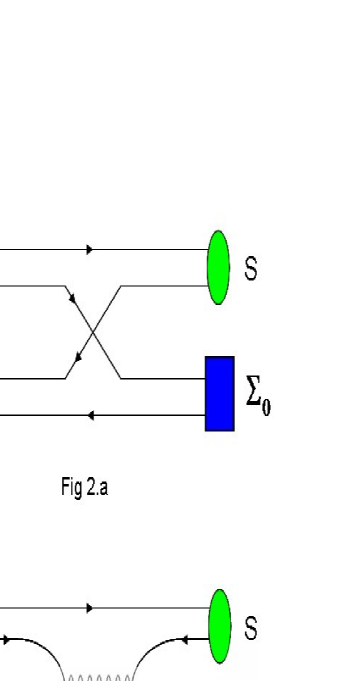
Figure 2: Dominant (2.a) and subdominant (2.b) contributions to the tetraquark-quarkonia mixing, corresponding to Eq. (34). At one vertex the $vev$’s for the scalar-isoscalar quarkonia fields, encoded in the matrix $\Sigma_{0}$ of Eq. (7), appears. As a consequence a tetraquark-quarkonia mixing is generated, whose strength is related to $\Sigma_{0}$, i.e. to the pion and kaon decay constants.

We depict the process corresponding to $\mathcal{L}_{mix}$ in Fig. 2, where the two diagrams resemble Figs 1.a and 1.b, but at one vertex the vacuum expectation matrix $\Sigma_{0}$ enters in the game. If $\Sigma_{0}$ vanishes, such terms vanish as well. It is noticeable that the decay-strengths parameters $c_{1}$ and $c_{2}$ also regulate the intensity of the mixing. In Eq. (23) and in Refs. [16, 17, 18] the scalar states below 1 GeV are interpreted as pure tetraquark states. The present analysis shows that such an assignment cannot be strictly valid because mixing occurs. We aim now to evaluate the intensity of this mixing in the isovector channel.

An important point is the following: in section 2.1 we discussed various arguments in favour of bare quarkonia masses well above $1$ GeV. At the same time in the Introduction and in Section 2.4 we recalled that the scalar diquark emerges a compact light object within different approaches (one-gluon exchange [1, 19], instantons [20, 21], NJL model and DSE [22, 23]). The s-wave tetraquark states arising by composition of a diquark and antidiquark (as expressed in Eq. (12) and (16)-(20)) is expected to have a mass below (or about) 1 GeV, as discussed in Sections 2.1 and 2.2 by means of phenomenological arguments and as suggested by the Lattice works of Refs. [24, 25, 26]. These facts lead us to consider the bare level ordering $M_{4q}<M_{\overline{q}q}.$

3.2.2 Mixing in the isovector channel

We analyze the mixing of the two neutral $a_{0}^{0}$ states, denoted as $a_{0}^{0}[4q]$ (from the tetraquark nonet $\mathcal{S}^{[4q]}$ of Eq. (16)-(20)) and as $a_{0}^{0}[\overline{q}q]$ (from the quarkonia nonet $\mathcal{S}$ of Table 1). The isovector channel is free from isoscalar-mixing (and glueball) complications, and is experimentally better known than the kaonic sector.

We isolate in $\mathcal{L}_{mix}$ of Eq. (34) the part concerning the neutral $a_{0}$ states:

$$\mathcal{L}_{\text{mix-}a_{0}^{0}}=2(c_{1}\alpha_{s}+c_{2}\alpha_{u})\left(a_{0}^{0}[4q]\cdot a_{0}^{0}[\overline{q}q]\right).$$ (35)

When including the kinematic and (bare) mass contributions one has to diagonalize the following Lagrangian:

$$\mathcal{L=}\frac{1}{2}\left(\partial_{\mu}a_{0}^{0}[4q]\right)^{2}+\frac{1}{2}\left(\partial_{\mu}a_{0}^{0}[\overline{q}q]\right)^{2}+\frac{1}{2}v^{t}\Omega v$$ (36)

where

$$v=\left(\begin{array}[]{c}a_{0}^{0}[4q]\\ a_{0}^{0}[\overline{q}q]\end{array}\right),\text{ }\Omega=\left(\begin{array}[]{cc}-M_{a_{0}^{0}[4q]}^{2}&2(c_{1}\alpha_{s}+c_{2}\alpha_{u})\\ 2(c_{1}\alpha_{s}+c_{2}\alpha_{u})&-M_{a_{0}^{0}[\overline{q}q]}^{2}\end{array}\right).$$ (37)

The orthogonal transformation matrix $B$, given by

$$B\Omega B^{t}=-diag\{M_{a_{0}(980)}^{2},M_{a_{0}(1470)}^{2}\}\text{ ,}$$ (38)

connects the bare tetraquark and quarkonia states to the physical ones:

$$\left(\begin{array}[]{c}a_{0}^{0}(980)\\ a_{0}^{0}(1470)\end{array}\right)=B\cdot\left(\begin{array}[]{c}a_{0}^{0}[4q]\\ a_{0}^{0}[\overline{q}q]\end{array}\right),\text{ }B=\left(\begin{array}[]{cc}\cos(\theta)&\sin(\theta)\\ -\sin(\theta)&\cos(\theta)\end{array}\right).$$ (39)

The physical masses read [27]:

$$M_{a_{0}(980)}=984.7\pm 1.2\text{ MeV and }M_{a_{0}(1450)}=1474\pm 19\text{ MeV.}$$ (40)

The decay rates for the decay channel $a_{0}(980)\rightarrow\eta\pi$ and $a_{0}(1450)\rightarrow\eta\pi$ are given by:

$$\Gamma_{a_{0}(980)\rightarrow\eta\pi}=\frac{p_{a_{0}(980)\rightarrow\eta\pi}}{8\pi M_{a_{0}(980)}^{2}}g_{{}_{a_{0}(980)\rightarrow\eta\pi}}^{2},\text{ }\Gamma_{a_{0}(1450)\rightarrow\eta\pi}=\frac{p_{a_{0}(1450)\rightarrow\eta\pi}}{8\pi M_{a_{0}(1450)}^{2}}g_{{}_{a_{0}(1450)\rightarrow\eta\pi}}^{2},$$ (41)

where $p_{a_{0}(980)\rightarrow\eta\pi}$ and $p_{a_{0}(1450)\rightarrow\eta\pi}$ represent the phase-space factors and the decay amplitudes $g_{{}_{a_{0}(980)\rightarrow\eta\pi}}$ and $g_{{}_{a_{0}(1450)\rightarrow\eta\pi}}$ are a superposition of the tetraquark and quarkonia contributions:

$$g_{{}_{a_{0}(980)\rightarrow\eta\pi}}^{2} = \left[g_{{}_{a_{0}[4q]\rightarrow\eta\pi}}\cos(\theta)+g_{{}_{a_{0}[\overline{q}q]\rightarrow\eta\pi}}\sin(\theta)\right]^{2},$$

$$g_{{}_{a_{0}(1450)\rightarrow\eta\pi}}^{2} = \left[-g_{{}_{a_{0}[4q]\rightarrow\eta\pi}}\sin(\theta)+g_{{}_{a_{0}[\overline{q}q]\rightarrow\eta\pi}}\cos(\theta)\right]^{2}.$$ (42)

The amplitude $g_{{}_{a_{0}[4q]\rightarrow\eta\pi}}$ is calculated from $\mathcal{L}_{\mathcal{S}^{[4q]}PP}$ of Eq. (21) and reads [18]:

$$g_{{}_{a_{0}[4q]\rightarrow\eta\pi}}=\frac{2c_{1}}{\sqrt{3}}\left[\sqrt{2}\cos(\theta_{P})+\sin(\theta_{P})\right]+\sqrt{\frac{2}{3}}c_{2}\left[\cos(\theta_{P})-\sqrt{2}\sin(\theta_{P})\right]$$ (43)

where $\theta_{P}=-9.95^{\circ}$ at tree-level [10, 49].

The quantity $g_{{}_{a_{0}[\overline{q}q]\rightarrow\eta\pi}}$ depends on the Lagrangian describing the decay of scalar quarkonia into pseudoscalar mesons, which we did not specify in this work. In the following we will treat it as a free parameter, see below.

We now turn the attention to the experimental informations about the coupling constants in Eq. (43). The coupling constant $g_{{}_{a_{0}(980)\rightarrow\eta\pi}}^{2}$ as extracted from experimental analyses varies between $5$ and $10$ GeV² [50]. We then consider the following three values in the above range:

$$g_{{}_{a_{0}(980)\rightarrow\eta\pi}}^{2}=5,\text{ }7.5,\text{ }10\text{ GeV}^{2}$$ (44)

which corresponds to $\Gamma_{a_{0}(980)\rightarrow\eta\pi}=65.8,$ $98.7$, $131.6$ MeV respectively. These values are compatible with the data reported by PDG [27], which are however not yet precise. By using

$$\Gamma_{a_{0}(980)}=\Gamma_{a_{0}(980)\rightarrow\overline{K}K}+\Gamma_{a_{0}(980)\rightarrow\eta\pi}\text{ and }\frac{\Gamma_{a_{0}(980)\rightarrow\overline{K}K}}{\Gamma_{a_{0}(980)\rightarrow\eta\pi}}=0.183\pm 0.024\text{ \cite[cite]{[\@@bibref{}{pdg}{}{}]},}$$

we obtain (ignoring the error on the last ratio): $\Gamma_{a_{0}(980)\rightarrow\eta\pi}=\Gamma_{a_{0}}/1.183.$ In PDG [27] the value $\Gamma_{a_{0}(980)}=50$-$100$ MeV is reported, thus implying $\Gamma_{a_{0}(980)\rightarrow\eta\pi}$ equal to $42.3$ and $84.6$ MeV respectively. The largest value $g_{{}_{a_{0}(980)\rightarrow\eta\pi}}^{2}=10$ GeV² seems disfavored and we regard it as an upper limit.

We now turn the attention to $g_{{}_{a_{0}(1450)\rightarrow\eta\pi}}^{2}.$ In Ref. [27] the averages for the following branching ratios are reported:

$$\frac{\Gamma_{a_{0}(1450)\rightarrow\eta^{\prime}\pi}}{\Gamma_{a_{0}(1450)\rightarrow\eta\pi}}=0.35\pm 0.16,\text{ }\frac{\Gamma_{a_{0}(1450)\rightarrow\overline{K}K}}{\Gamma_{a_{0}(1450)\rightarrow\eta\pi}}=0.88\pm 0.23.$$

The full width amounts to $\Gamma_{a_{0}(1450)}=265\pm 13$ MeV. The contribution of the two-pseudoscalar decays to the full width is unknown. By assuming it to be dominant, and thus that the $\omega\rho$ mode is suppressed, we obtain $\Gamma_{a_{0}(1450)\rightarrow\eta\pi}\simeq 119$ MeV, corresponding to $g_{{}_{a_{0}(1450)\rightarrow\eta\pi}}^{2}{}\simeq 10.4$ GeV${}^{2}.$ We do not include errors because we ignore the contribution of the $\omega\rho$ decay to the full width. Furthermore, the experimental result $\Gamma_{a_{0}(1450)\rightarrow\omega\rho}/\Gamma_{a_{0}(1450)\rightarrow\eta\pi}=10.7\pm 2.3$ reported in Ref. [51] would indicate a dominant $\omega\rho$ mode. This value is however not listed as an average or fit in [27]. We will consider the value

$$g_{{}_{a_{0}(1450)\rightarrow\eta\pi}}^{2}=10.4\text{ GeV}^{2}\text{,}$$ (45)

being aware that it could be smaller.

We now turn to the evaluation of the mixing angle. We consider the theoretical coupling $g_{{}_{a_{0}[\overline{q}q]\rightarrow\eta\pi}}$ of Eq. (42) as a free parameter, thus we are left with five parameters: $\{c_{1},c_{2},M_{a_{0}^{0}[4q]},M_{a_{0}^{0}[\overline{q}q]},g_{{}_{a_{0}[\overline{q}q]\rightarrow\eta\pi}}\}.$ We fix the ratio $c_{2}/c_{1}=0.62$ as obtained in [18], where the light scalar are interpreted as tetraquark states. Although this choice cannot be a priori justified, we will then vary the ratio $c_{2}/c_{1}$ checking the dependence of the results on it.

We fix the remaining four parameters to the physical masses of Eq. (40), to the intermediate value $g_{{}_{a_{0}(980)\rightarrow\eta\pi}}^{2}=7.5$ GeV² of Eq. (44) and to Eq. (45).

By using the bare level ordering $M_{a_{0}^{0}[4q]}<M_{a_{0}^{0}[\overline{q}q]}$ the parameters are determined as (values in GeV, ratio $c_{2}/c_{1}=0.62$ fixed):

$$\left|c_{1}\right|=0.96\text{, }M_{a_{0}^{0}[4q]}=1.01,\text{ }M_{a_{0}^{0}[\overline{q}q]}=1.45,\text{ }g_{{}_{a_{0}[\overline{q}q]\rightarrow\eta\pi}}=3.75\text{ .}$$ (46)

corresponding to a quarkonium amount in the resonance $a_{0}(980)$:

$$(\sin\theta)^{2}=4.93\%\text{ }.$$ (47)

According to our result the resonance $a_{0}(980)$ has a by far dominant tetraquark substructure and only a small quarkonium amount. Similarly, the resonance $a_{0}(1450)$ has a dominant quarkonium substructure with a small $4.93\%$ tetraquark content. The mixing between the tetraquark and quarkonia states turns out to be small.

To have used $c_{2}/c_{1}=0.62$ from [18] is then justified a posteriori. Anyway, when varying the ratio $c_{2}/c_{1}$ and the couplings of Eqs. (44)-(45) the results show a stable behavior: the mixing turns out to be small for all reasonable parameter choices, see Appendix B.

Notice that we cannot determine the sign of the mixing angle $\theta$ and $c_{1}.$ In fact, we have no information about the sign of $g_{{}_{a_{0}(1450)\rightarrow\eta\pi}}$ and $g_{{}_{a_{0}(980)\rightarrow\eta\pi}}$ from experiment. For this reason the modulus $\left|c_{1}\right|$ is reported in Eq. (46). If $c_{1}>0,$ then $\theta>0$ and vice-versa. The two possibilities are however indistinguishable here.

3.2.3 Further discussion

Some comments are in other:

a) In the kaonic sector the situation is similar. For instance, the part of the Lagrangian $\mathcal{L}_{mix}$ (34) describing the $k^{-}[4q]$-$K_{0}^{-}[\overline{q}q]$ mixing reads:

$$\mathcal{L}_{\text{mix-}k}=-(2c_{1}\alpha_{u}+c_{2}(\alpha_{u}+\alpha_{s}))\left(k^{-}[4q]\cdot K_{0}^{+}[\overline{q}q]\right).$$ (48)

By using the solution reported in Eq. (46) and the masses $M_{k(800)}\simeq 800$ MeV and $M_{K_{0}(1430)}=1414\pm 6$ MeV we obtain a quarkonium amount in $k(800)$ of the order of $3\%,$ i.e. very small. As a consequence, the state $K_{0}(1430)$ has a dominant quarkonium content. The corresponding bare masses of the tetraquark and quarkonia states are $M_{k[4q]}=823$ MeV and $M_{K[\overline{q}q]}=1400$ MeV, thus only slightly shifted from the physical masses.

Let us turn to the problematic $\pi K$-decay of the two resonances: the smallness of the mixing allows us to consider the approximate relations $g_{k(800)\rightarrow\pi K}\simeq g_{k[4q]\rightarrow\pi K}$ ($=\sqrt{3}(\sqrt{2}c_{1}+c_{2}/\sqrt{2})$ as evaluated in [18]) and $g_{K(1430)\rightarrow\pi K}\simeq g_{K[\overline{q}q]\rightarrow\pi K}.$ Using the parameters of (46) one finds $\Gamma_{k(800)\rightarrow\pi K}\simeq 130$ MeV. The uncertainty on the decay strengths $c_{1}$ and $c_{2}$ allows for a width between $100$ and $220$ MeV. The values in this range are smaller than the present (not yet conclusive) experimental value of about $600$ MeV [27]. We refer to the discussions about the experimental caveats in Ref. [31], where it is also pointed out that quarkonium, molecular or tetraquark interpretations all fail in reproducing the large width of $k(800)$. Meson-meson interaction governed by chiral symmetry as presented in Ref. [15] can play an important role to explain the large width of $k(800)$. It is important to stress that also the decay $K(1430)\rightarrow\pi K$, evaluated in Ref. [10], turns out to be smaller than the present data of a factor 4. This problem has been analyzed in detail in Ref. [10] and is rather model-independent. Further work both on theoretical and experimental sides is clearly needed to fit all the properties of the kaonic states $k(800)$ and $K_{0}(1430)$ in a unified picture.

b) We report the mixing Lagrangian in the isoscalar sector in terms of the bare states $\sigma_{B}[4q]=\frac{1}{2}[u,d][\overline{u},\overline{d}]$, $f_{B}[4q]=\frac{1}{2\sqrt{2}}([u,s][\overline{u},\overline{s}]+[d,s][\overline{d},\overline{s}])$ and $N=\sqrt{\frac{1}{2}}(\overline{u}u+\overline{d}d),$ $S=\overline{s}s$ :

$$\mathcal{L}_{\text{mix-iso}} = 2(c_{1}\alpha_{s}+c_{2}\alpha_{u})Nf_{B}[4q]+2\sqrt{2}(c_{1}\alpha_{u}+c_{2}\alpha_{s})Sf_{B}[4q]$$ (49)

$$+2\sqrt{2}(c_{1}+c_{2})\alpha_{u}N\sigma_{B}[4q].$$

The intensity of the mixing is of the same order of magnitude of the isovector and isodoublet channel, that is small. The system is then complicated by internal mixing terms like $\sigma_{B}f_{B}$ and $NS$ and glueball mixing, which lead to the resonances $f_{0}(600)$ and $f_{0}(980)$ below 1 GeV, and to $f_{0}(1370),$ $f_{0}(1500)$ and $f_{0}(1710)$ above 1 GeV. Here we do not analyze this system quantitatively (see Ref. [36] for such a study). However, the tetraquark-quarkonia mixing is small as verified in the isovector and isodoublet channels, thus it is still valid to deal with two separated tetraquark and quarkonia nonets with the scalar glueball intruding in the scalar-isoscalar quarkonia sector between 1 and 2 GeV. We therefore expect smaller mixing than in Ref. [36].

c) We did not take into account the momentum-dependence of the theoretical amplitudes $g_{{}_{a_{0}[\overline{q}q]\rightarrow\eta\pi}}$ and $g_{{}_{a_{0}[4q]\rightarrow\eta\pi}}.$ For instance, within a chiral perturbation theory framework the quantity $g_{{}_{a_{0}[\overline{q}q]\rightarrow\eta\pi}}$ has a (dominant) momentum-squared $p^{2}$ dependence of the form $g_{{}_{a_{0}[\overline{q}q]\rightarrow\eta\pi}}\propto(p^{2}-M_{\pi}^{2}-M_{\eta}^{2})$ [10]. When including such form in the calculation the results are similar. In general (reasonable) momentum dependence does not change the picture, see Appendix B.

d) One of the basic starting points of the evaluation of the mixing has been the bare level ordering $M_{a_{0}^{0}[4q]}<M_{a_{0}^{0}[\overline{q}q]}.$ The reasons for this choice have been listed in Sections 2.1 and 3.2.1. Here we notice that solutions are possible also for the reversed bare level ordering $M_{a_{0}^{0}[4q]}>M_{a_{0}^{0}[\overline{q}q]},$ for which the quarkonium content is dominant in $a_{0}(980).$ Although the case $M_{a_{0}^{0}[4q]}>M_{a_{0}^{0}[\overline{q}q]}$ seems unlikely for the above mentioned discussions, it cannot be ruled out.

e) The interaction Lagrangian $\mathcal{L}_{c.i.}$ of Eq. (29) contains the dominant and subdominant terms in large-$N_{c}$ expansion. Further large-$N_{c}$ suppressed terms and flavor-symmetry breaking terms were not included in the present analysis. Although they can quantitatively influence the results, they are not believed to change the qualitative picture emerging from this work.

3.3 Tetraquark condensates

3.3.1 Vacuum expectation values and estimation of tetraquark condensates

The term $\mathcal{L}_{4q\text{-}cond}$ of Eq. (33) is linear in $\mathcal{S}^{[4q]}$ and quadratic in $\Sigma_{0}$. It explicitly reads:

$$\mathcal{L}_{4q\text{-cond}} = c_{1}Tr\left[D\Sigma_{0}D^{\dagger}\Sigma_{0}\right]+c_{2}Tr\left[DD^{\dagger}\Sigma_{0}^{2}\right]$$ (50)

$$= 2(c_{1}+c_{2})\alpha_{u}^{2}\sigma_{B}[4q]+\sqrt{2}\left(2c_{1}\alpha_{u}\alpha_{s}+c_{2}(\alpha_{u}^{2}+\alpha_{s}^{2})\right)f_{B}[4q]$$

where in the second line the flavor-trace has been performed and a linear dependence in the isoscalar fields $\sigma_{B}[4q]$ and $f_{B}[4q]$ is found. This implies non-zero vacuum expectation values for these two (bare) fields:

$$\left\langle\sigma_{B}[4q]\right\rangle=\frac{2(c_{1}+c_{2})\alpha_{u}^{2}}{M_{\sigma_{B[4q]}}^{2}},\text{ }\left\langle f_{B}[4q]\right\rangle=\sqrt{2}\frac{2c_{1}\alpha_{u}\alpha_{s}+c_{2}(\alpha_{u}^{2}+\alpha_{s}^{2})}{M_{f_{B}[4q]}^{2}},$$ (51)

where $M_{\sigma_{B}[4q]}$ and $M_{f_{B}[4q]}^{2}$ refer to the (bare) tetraquark masses of the states $\sigma_{B}[4q]$ and $f_{B}[4q].$

The non-zero vacuum expectation value ($vev$) of the nonet $\mathcal{S}^{[4q]}$ (16)-(20) reads:

$$\left\langle\mathcal{S}_{ij}^{[4q]}\right\rangle=\beta_{i}\delta_{ij},\text{ }\beta_{1}=\beta_{2}=\frac{\left\langle f_{B}[4q]\right\rangle}{\sqrt{2}},\text{ }\beta_{3}=\left\langle\sigma_{B}[4q]\right\rangle.$$ (52)

We can estimate the corresponding tetraquark condensate following the discussion of [34]:

$$\left|\left\langle\frac{1}{2}\left(\varepsilon_{ikl}\overline{q}_{k}^{t}C\gamma^{5}\overline{q}_{l}\right)\left(\varepsilon_{jrm}q_{r}^{t}C\gamma^{5}q_{m}\right)\right\rangle\right|\sim\Lambda_{QCD}^{5}\beta_{i}\delta_{ij}.$$ (53)

The scale-factor $\Lambda_{QCD}^{5}$ enters on dimensional ground. In virtue of the flavour content of the fields $\sigma_{B}[4q]=\frac{1}{2}[u,d][\overline{u},\overline{d}]$ and $f_{B}[4q]=\frac{1}{2\sqrt{2}}([u,s][\overline{u},\overline{s}]+[d,s][\overline{d},\overline{s}])$ and using the parameter set of Eq. (46) together with $\Lambda_{QCD}\sim 0.25$ GeV we obtain:

$$\left|\left\langle\frac{1}{2}[u,d][\overline{u},\overline{d}]\right\rangle\right|\sim\Lambda_{QCD}^{5}\beta_{3}\simeq 3.1\cdot 10^{-5}\text{ GeV}^{6}$$ (54)

$$\left|\left\langle\frac{1}{2}[u,s][\overline{u},\overline{s}]\right\rangle\right|=\left|\left\langle\frac{1}{2}[d,s][\overline{d},\overline{s}]\right\rangle\right|\sim\Lambda_{QCD}^{5}\beta_{1}\simeq 1.9\cdot 10^{-5}\text{ GeV}^{6}$$ (55)

where the typical bare tetraquark masses $M_{\sigma_{B}[4q]}\sim 0.65$ GeV and $M_{f_{B}[4q]}^{2}$ $\sim 1$ GeV have been employed [18]. The precise value of the bare tetraquark masses is not relevant for our estimation. It is interesting to notice that the magnitude of the condensates is similar to [34].

3.3.2 Self-consistency problem

The tetraquark nonet $\mathcal{S}^{[4q]}$ acquires non-zero $vev$’s $\left\langle\mathcal{S}_{ij}^{[4q]}\right\rangle=\beta_{i}\delta_{ij}$ (Eqs. (51)-(52)). Then, one has to shift the nonet as $\mathcal{S}_{ij}^{[4q]}\rightarrow\mathcal{S}_{ij}^{[4q]}+\beta_{i}\delta_{ij}$ and substitute it back into the Lagrangian (30). In particular, when considering the mixing term of Eq. (49) the shift generates linear terms in the quarkonium scalar-isoscalar fields $N=\sqrt{\frac{1}{2}}(\overline{u}u+\overline{d}d)$ and $S=\overline{s}s$ :

$$\mathcal{L}_{\text{mix-iso}}\rightarrow 2\sqrt{2}(c_{1}\alpha_{s}+c_{2}\alpha_{u})N\beta_{1}+4\sqrt{2}(c_{1}\alpha_{u}+c_{2}\alpha_{s})S\beta_{1}+2\sqrt{2}(c_{1}+c_{2})\alpha_{u}N\beta_{3}+...$$ (56)

Then, these linear terms modify the vacuum expectation values for the scalar quarkonium nonet of Eq. (5) as:

$$\left\langle\mathcal{S}_{11}\right\rangle=\left\langle\mathcal{S}_{22}\right\rangle=\alpha_{u}\rightarrow\alpha_{u}+2\frac{(c_{1}\alpha_{s}+c_{2}\alpha_{u})\beta_{1}+(c_{1}+c_{2})\alpha_{u}\beta_{3}}{M_{N}^{2}}$$ (57)

$$\left\langle\mathcal{S}_{33}\right\rangle=\alpha_{s}\rightarrow\alpha_{s}+\frac{4\sqrt{2}(c_{1}\alpha_{u}+c_{2}\alpha_{s})}{M_{S}^{2}}\beta_{1}$$ (58)

where $M_{N}$ and $M_{S}$ refer to the bare quarkonia masses; we employ the typical values $M_{N}\sim 1.3$ GeV and $M_{S}\sim 1.6$ GeV [10].

The modification of the vacuum expectation values of the scalar quarkonia fields acknowledges the problem mentioned in Section 3.1: the minimum $\Sigma_{0}$ of the potential $V_{0}+V_{SB}$ is not anymore a minimum of our entire potential $V_{0}+V_{SB}-\mathcal{L}_{\mathcal{S}^{[4q]}\Sigma\Sigma}.$

We have to take it into account when evaluating the values of $\alpha_{u}$ and $\alpha_{s}$ from Eq. (6). When using the modified expressions (57)-(58) in the Eq. (5), here rewritten as

$$\left\langle\mathcal{S}_{11}\right\rangle+\left\langle\mathcal{S}_{22}\right\rangle=\sqrt{2}F_{\pi}\text{, }\left\langle\mathcal{S}_{11}\right\rangle+\left\langle\mathcal{S}_{33}\right\rangle=\sqrt{2}F_{K}\text{ ,}$$ (59)

the constants $\alpha_{u}$ and $\alpha_{s}$ change as follows (the parameter set of Eq. (46) and the above listed scalar masses are employed):

$$\alpha_{u}=\frac{F_{\pi}}{\sqrt{2}}\rightarrow\frac{F_{\pi}}{\sqrt{2}}(1-0.11)\text{ ,}$$ (60)

$$\alpha_{s}=-\frac{F_{\pi}}{\sqrt{2}}+\sqrt{2}F_{K}\rightarrow\left(-\frac{F_{\pi}}{\sqrt{2}}+\sqrt{2}F_{K}\right)(1-0.06)\text{ .}$$ (61)

The corrections to the vacuum expectation values are $11\%$ and $6\%$ respectively, that is safely small. The results of the mixing evaluation in Section 3.2 and in Appendix B are therefore confirmed. Indeed, the imprecise knowledge of the experimental coupling constants of Eqs. (44)-(45) generates a larger uncertainty than the neglect of the $vev$’s corrections. The smallness of the latter originates from factors of the kind $(\sqrt{2}\alpha_{u}/M_{scalar})^{2}\sim(F_{\pi}/M_{scalar})^{2}$ in Eqs. (57)-(58), where $M_{scalar}\sim 1$ GeV refers to the typical order of magnitude for the bare scalar tetraquark and quarkonia fields.

One should then proceed iteratively, by shifting again the $vev$ of the scalar-quarkonia fields according to Eqs. (57)-(58) and subsequently finding in the Lagrangian the new linear terms in the scalar tetraquark fields (which arise from the scalar-tetraquark mixing terms); in turn, this procedure allows to determine the next-to-leading order correction to the tetraquark $vev$ of Eq. (52). For instance, by using the new ‘alfa-values’ of Eqs. (60)-(61) and calculating the next-order correction to the $vev$ $\beta_{3},$ a slight increase of $4\%$ is found, a small fraction which does not change the results of the previous subsection about the tetraquark condensates. This result is expected because the n-th correction involves factors like $(F_{\pi}/M_{scalar})^{2n}$, thus decreasing very fast. Naively, the minimum of the extended potential $V_{0}+V_{SB}-\mathcal{L}_{\mathcal{S}^{[4q]}\Sigma\Sigma}$ is close to the minimum $\Sigma_{0}$ of $V_{0}+V_{SB}.$ In the next subsection an explicit study of this issue by means of a simple toy model is performed avoiding complicated algebraic expressions. Notice that the iterative process is the unique way to proceed because the exact form of the potential $V_{0}+V_{SB}$ is not specified.

The shift of the tetraquark nonet also induces contributions to the pseudoscalar and scalar quarkonia masses (terms $\mathcal{L}_{\mathcal{S}^{[4q]}PP}$ and $\mathcal{L}_{\mathcal{S}^{[4q]}SS}$ in Eq. (33)). This fact has no influence in this work because we do not evaluate the bare quarkonia and tetraquark masses.

3.3.3 Toy potential

Let us consider only the light quarks $u$ and $d$: as well known, chiral symmetry invariance under $SU_{R}(2)\times SU_{L}(2)$ is fulfilled by considering $\Sigma=N\tau^{0}+i\pi^{i}\tau^{i},$ where $N\equiv\overline{n}n=\sqrt{1/2}(\overline{u}u+\overline{d}d)$ is the isoscalar-quarkonium field, $\pi^{i}$ the pseudoscalar pionic fields and $\tau^{i}$ the 3 Pauli matrices ($\tau^{0}$ is the $2\times 2$ identity matrix).

In the $SU(2)$ limit only one scalar-diquark field survives: $\varphi=\sqrt{\frac{1}{2}}\varepsilon_{jk}q_{j}^{t}C\gamma^{5}q_{k}.$ The scalar-diquark matrix is given by $D=\varphi A$ where $A=i\tau^{2}.$ Thus, we are left with only one tetraquark field: $T=\sigma_{B}[4q]=\frac{1}{2}[u,d][\overline{u},\overline{d}].$

The Lagrangian $\mathcal{L}_{\mathcal{S}^{[4q]}\Sigma\Sigma}$ in Eq. (30) reduces to the very simple form:

$$\mathcal{L}_{\mathcal{S}^{[4q]}\Sigma\Sigma}\rightarrow gT\left(N^{2}+\overrightarrow{\pi}^{2}\right),\text{ }g=c_{1}+c_{2}.$$ (62)

(In the $SU(2)$ case the expressions for the dominant and subdominant terms in large-$N_{c}$ expansion coincide). For illustrative purpose we use the usual Mexican-hat potential $V_{0}=\frac{\lambda}{4}(N^{2}+\overrightarrow{\pi}^{2}-F^{2})^{2}$ and neglect $V_{SB}.$ Thus, the toy potential of the reduced $SU(2)$-problem reads:

$$V_{\text{toy}}=\frac{\lambda}{4}(N^{2}+\overrightarrow{\pi}^{2}-F^{2})^{2}+\frac{1}{2}M_{T}^{2}T^{2}-gT\left(N^{2}+\overrightarrow{\pi}^{2}\right)$$ (63)

where a mass-term for the tetraquark field has been included.

The minimum of $V_{0}$ is at $\{N_{0}=F,\overrightarrow{\pi}=\overrightarrow{0}\}.$ By expanding around this point, i.e. shifting $N\rightarrow F+N,$ the quantity $\mathcal{L}_{\mathcal{S}^{[4q]}\Sigma\Sigma}$ in the SU(2) limit generates analogous terms to those discussed throughout this section:

$$\mathcal{L}_{\mathcal{S}^{[4q]}\Sigma\Sigma}\rightarrow gT\left(N^{2}+\overrightarrow{\pi}^{2}\right)=gT(N^{2}+\overrightarrow{\pi}^{2}+2FN+F^{2})$$ (64)

In fact, we recognize the tetraquark-mesons decay terms, the mixing term (whose strength amounts to $2gF$) and the linear term in the field  $T$.

But the minimum of $V_{0}$ is not the minimum of $V_{\text{toy}}.$ The corresponding minimum point of $V_{\text{toy}}$, denoted as $P_{\min}=\{N_{0},T_{0},\overrightarrow{\pi}=\overrightarrow{0}\},$ can be analytically calculated:

$$N_{0} = \frac{F}{\sqrt{1-\frac{2g^{2}}{\lambda M_{T}^{2}}}}=F\left(1+\frac{g^{2}}{\lambda M_{T}^{2}}+...\right),\text{ }$$ (65)

$$T_{0} = \frac{g}{M_{T}^{2}}N_{0}^{2}=\frac{g}{M_{T}^{2}}\frac{F^{2}}{1-\frac{2g^{2}}{\lambda M_{T}^{2}}}=\frac{gF^{2}}{M_{T}^{2}}\left(1+\frac{2g^{2}}{\lambda M_{T}^{2}}+...\right).$$ (66)

When $g=0$ we reobtain the minimum at $N_{0}=F$ and $T_{0}=0.$ If the term $g^{2}/\lambda M_{T}^{2}$ entering in the expansions is small, one simply has small corrections to the value $N_{0}=F$ . The toy-model clarifies what kind of correction terms one evaluates in the iterative process sketched in the previous subsection leading to Eqs. (60)-(61).

The bare mass of the field $N$ and the mixing strength can be also exactly evaluated by expanding around the minimum $P_{\min}$:

$$M_{N}^{2}=\left(\frac{\partial^{2}V_{\text{toy}}}{\partial N^{2}}\right)_{P=P_{\min}}=\frac{2\lambda F^{2}}{1-\frac{2g^{2}}{\lambda M_{T}^{2}}},\text{ }\left(\frac{\partial^{2}V_{\text{toy}}}{\partial N\partial T}\right)_{P=P_{\min}}=-2gN_{0}.$$ (67)

Let us estimate the corrections. The parameter $\lambda$ at first order is: $\lambda\simeq M_{N}^{2}/2F^{2}.$ This value is accurate if $\frac{2g^{2}}{\lambda M_{T}^{2}}\simeq\frac{4g^{2}F^{2}}{M_{T}^{2}M_{N}^{2}}<<1.$ The condition is satisfied in our case. In fact, using the typical values $g\sim 1.5$ GeV (as in Eq. (46)) $F\sim F_{\pi},$ $M_{T}\sim 0.65$ GeV and $M_{N}\sim 1.3$ GeV one has $\frac{4g^{2}F_{\pi}^{2}}{M_{T}^{2}M_{N}^{2}}\simeq 0.1$; we also see the appearance of factor like $(F_{\pi}/M_{scalar})^{2}$ in the Taylor expansion, as already discussed in Section 3.2.

4 Summary and conclusions

This work aimed to study the implications of Jaffe’s tetraquark states as a necessary component to correctly interpret the scalar low-energy QCD sector. We summarize the relevant points.

a) The scalar and the pseudoscalar quarkonia nonets are introduced in the usual fashion. We did not specify the potential for these fields, but we solely assumed chiral symmetry breaking to occur, thus non-vanishing $vev$’s for the isoscalar quarkonia fields, in turn related to the pion and kaon decay constants $F_{\pi}$ and $F_{K},$ are generated. The bare scalar quarkonia masses are set above 1 GeV (in accord with the Lattice study of Ref. [41, 45, 26]), where the other p-wave nonets of axial-vector and tensor mesons lie.

b) The scalar diquark in the flavor $\left(\overline{3}_{F}\right)$and color $\left(\overline{3}_{C}\right)$ antitriplet configurations is a compact and stable object, thus a good candidate for the basic building block of the light scalar mesons, which naturally emerge as a tetraquark scalar nonet. This assignment is in agreement with the mass-degeneracy of $a_{0}(980)$ and $f_{0}(980)$, their large $\overline{K}K$ decay strengths and their non-quarkonia behavior for large-$N_{c}$ analysis. These facts, together with point (a), support the bare level ordering $M_{4q}<M_{\overline{q}q}.$

c) In a chiral framework the $\left(\overline{3}_{F},\overline{3}_{C}\right)$ pseudoscalar diquark is introduced as the chiral partner of the scalar diquark. Chiral symmetry breaking driven by instantons predicts a strong attraction in the scalar channel and a repulsion in the pseudoscalar one. This fact makes the pseudoscalar diquark heavier and loosely bound, thus we do not consider it as a relevant constituent for the light meson spectroscopy. For instance, an extra non-quarkonia nonet built out two pseudoscalar diquark is not seen in the spectrum below 2 GeV.

d) A tetraquark-quarkonia interaction Lagrangian invariant under $SU_{R}(3)\times SU_{L}(3)\times U_{A}(1)$ is written down at the leading and subleading order in the large-N_c expansion. Both scalar and pseudoscalar diquark constituents enter in its expression. Then, in virtue of point (c) only the scalar diquark and the corresponding tetraquark nonet are taken into account.

e) The $\chi SB$ of point (a) generates a mixing term among the scalar quarkonia and tetraquark nonet. The corresponding mixing strengths are a linear combination of $F_{\pi}$ and $F_{K}$ and the tetraquark decay strengths $c_{1}$ and $c_{2},$ which parametrize the processes of Figs. 1.a and 1.b. The mixing is then evaluated in the isovector channel: $a_{0}(980)$ is mainly a Jaffe’s tetraquark state, with a small quarkonium amount $(\lesssim 10\%),$ and $a_{0}(1450)$ has a dominant quarkonium content. The results are similar in the kaonic sector and are stable under changes of the employed parameters, as long as the bare level ordering $M_{4q}<M_{\overline{q}q}$ holds.

f) The $\chi SB$ at a quarkonia level induces also linear terms in the isoscalar tetraquark fields, thus non-vanishing $vev$’s for the latter emerge. They are also related to the magnitude of corresponding four-quark condensate(s), whose values have been estimated about $2$-$3\cdot 10^{-5}$ GeV⁶. As a last step a self-consistency check about the minimum of scalar-isoscalar fields has been done and a simple toy-model for the reduced $SU(2)$ problem discussed.

We found a substantial separation of the tetraquark states (below 1 GeV) and quarkonia states (between 1-2 GeV, where the scalar glueball intrudes in the isoscalar sector). The confirmation of the falsification of this scenario is an important issue of low-energy hadronic QCD. Furthermore, decays of heavy states in the charmonia region involve the scalar mesons below 2 GeV. Thus, the correct interpretation of the latter is a crucial step for the analysis of the decays of charmonia and heavy-glueball states, which according to Lattice QCD are believed to show up in the mass region between 3-5 GeV [52], in turn related to the planed experimental search of PANDA at FAIR [53].

As an interesting development, the analysis of electromagnetic decay of (and into) vector meson such as $V\rightarrow S^{[4q]}\gamma$ [54] and $S^{[4q]}\rightarrow V\gamma$ [55] within a phenomenological composite Lagrangian can constitute a useful step in disentangling the nature of the light scalar states below 1 GeV and is planned as a future work. Along the same line, possible interactions involving the experimentally well-known tensor mesons within a composite approach as in [56] can also be performed.

Appendix A Nonets and their transformation

Out of the introduced diquarks we can (formally) identify 4 nonets, with definite properties under chiral transformations. We first consider the matrix of tetraquark states $T$ (analogous to $\widehat{\Phi}$ in [35] and $M^{\prime}$ in [34]):

$$T_{ij}=\sqrt{2}\varphi_{i}^{L\dagger}\varphi_{j}^{R};\text{ }T=T^{S}+iT^{P},\text{ }$$ (68)

which constitutes of a scalar and a pseudoscalar nonet of tetraquark states given by the Hermitian matrices:

$$T_{ij}^{S}=\frac{1}{\sqrt{2}}\left(\widetilde{\varphi}_{i}^{\dagger}\widetilde{\varphi}_{j}-\varphi_{i}^{\dagger}\varphi_{j}\right),\text{ }T_{ij}^{P}=\frac{i}{\sqrt{2}}\left(\varphi_{i}^{\dagger}\widetilde{\varphi}_{j}-\widetilde{\varphi}_{i}^{\dagger}\varphi_{j}\right)\text{ .}$$ (69)

The matrices $T,$ $T^{S}$ and $T^{P}$ transform as $\Sigma,$ $S$ and $P$ in Table 1, except for the $U_{A}(1)$ transformation, which now reads $T\rightarrow e^{-4i\nu}T$. In particular, for chiral transformations: $T\rightarrow LTR^{\dagger}$. Notice that the scalar nonet $\mathcal{S}^{[4q]}$ of Eqs. (12) and (23) is now a part of $T^{S}$. In the chiral context the scalar nonet $T^{S}$ is an admixture of both diquarks. In [30, 35] the tetraquark-quarkonia mixing occurs via the chirally invariant (but not $U_{A}(1)$ invariant) term

$$\mathcal{L}_{\text{mix}}=e\cdot Tr[\Sigma T^{\dagger}+T\Sigma^{\dagger}]$$ (70)

where $e$ is a free parameter.

Other two tetraquark meson nonets can be formed:

$$T_{ij}^{R}=\sqrt{2}\varphi_{i}^{R\dagger}\varphi_{j}^{R},\text{ }T_{ij}^{L}=\sqrt{2}\varphi_{i}^{L\dagger}\varphi_{j}^{L}$$ (71)

which under chiral transformations transform as $T^{R}\rightarrow RT^{R}R^{\dagger}$ and $T^{L}\rightarrow LT^{R}L^{\dagger},$ i.e. such as quark’s left and right currents, connected to vector and axial-vector mesons. In the present context we still deal with scalar and pseudoscalar tetraquark states, which we denote as $\Pi^{S}$ and $\Pi^{P}$:

$$\Pi^{S} = \frac{1}{2}(T^{R}+T^{L});\text{ }\Pi_{ij}^{S}=\frac{1}{\sqrt{2}}\left(\widetilde{\varphi}_{i}^{\dagger}\widetilde{\varphi}_{j}+\varphi_{i}^{\dagger}\varphi_{j}\right)$$ (72)

$$\Pi^{P} = \frac{1}{2}(T^{R}-T^{L});\text{ }\Pi_{ij}^{P}=\frac{1}{\sqrt{2}}\left(\varphi_{i}^{\dagger}\widetilde{\varphi}_{j}+\widetilde{\varphi}_{i}^{\dagger}\varphi_{j}\right)$$ (73)

The scalar and pseudoscalar nonets $\Pi^{S}$ and $\Pi^{P}$ transform as vector and axial-vector under chiral transformation. Out of a quark and an antiquark such scalar and pseudoscalar objects do not exist because they vanish identically (direct product $P_{R}\cdot P_{L}=0$ in the expression for the currents). They are however possible for tetraquark states: four nonets can be then formed.

After chiral symmetry breaking at a diquark level occurs, there is no reason that the physical nonets are those listed in the present Appendix. The scalar nonets $T^{S}$ and $\Pi^{S}$ can mix and split. This fact resembles the flavour wave functions of the vector mesons $\omega$ and $\phi$, where the quark mass splitting generates a separation of $(u,d)$ and $s$ quark dynamics. We assumed that the splitting is large enough to generate two separated nonets of scalar and pseudoscalar diquark constituents:

$$T^{S},\text{ }\Pi^{S}\rightarrow\mathcal{S}^{[4q]}=\varphi_{i}^{\dagger}\varphi_{j},\text{ }\widetilde{\varphi}_{i}^{\dagger}\widetilde{\varphi}_{j}$$ (74)

The scalar nonet $\widetilde{\varphi}_{i}^{\dagger}\widetilde{\varphi}_{j}$ does not show up in the spectrum below 2 GeV. It could be heavier, too broad or simply not realized in nature. Here we simply concentrated on $\mathcal{S}^{[4q]}.$ A more quantitative analysis of the splitting of scalar and pseudoscalar diquarks would represent an interesting subject on its own.

Appendix B Results for parameter variation

We evaluate the quarkonium amount in the resonance $a_{0}(980),$ represented by the quantity $\sin^{2}\theta,$ for different choices of the parameters. We consider all three values for $g_{{}_{a_{0}(980)\rightarrow\eta\pi}}^{2}=5$, $7.5$, $10$ GeV² listed in Eq. (44). We first employ $g_{{}_{a_{0}(1450)\rightarrow\eta\pi}}^{2}=10.4$ GeV² and we consider different values for the ratio $c_{2}/c_{1}.$ (The value $c_{2}/c_{1}=1$ would imply large-$N_{c}$ violation. Here it is used to show the stability of the results under changes of this ratio).

Table 4: $\sin^{2}\theta$ when varying $g_{{}_{a_{0}(980)\rightarrow\eta\pi}}^{2}$ and $\frac{c_{2}}{c_{1}}.$

($g_{{}_{a_{0}(1450)\rightarrow\eta\pi}}^{2}=10.4$ GeV²)

($\frac{c_{2}}{c_{1}}=\frac{1}{3}$) ($\frac{c_{2}}{c_{1}}=0.62$) ($\frac{c_{2}}{c_{1}}=1$) $g_{{}_{a_{0}(980)\rightarrow\eta\pi}}^{2}$ (GeV²) $\sin^{2}\theta$ $\sin^{2}\theta$ $\sin^{2}\theta$ 5 3.23% 3.22% 3.22% 7.5 4.82% 4.81% 4.80% 10 6.40% 6.39% 6.38%

Notice that the dependence on the ratio $c_{2}/c_{1}$ is extremely weak.

As stressed in Section 3.2.2 the value for $g_{{}_{a_{0}(1450)\rightarrow\eta\pi}}^{2}$ can be smaller than $10.4$ GeV${}^{2}.$ We evaluate $\sin^{2}\theta$ for $g_{{}_{a_{0}(1450)\rightarrow\eta\pi}}^{2}=5.2$ GeV${}^{2}.$ This value corresponds to a width four times smaller: $\Gamma_{a_{0}(1450)\rightarrow\eta\pi}\simeq 119/4=29.75$ MeV, probably to small. It can be regarded as a lower limit.

Table 5: $\sin^{2}\theta$ when varying $g_{{}_{a_{0}(980)\rightarrow\eta\pi}}^{2}$ and $\frac{c_{2}}{c_{1}}.$

($g_{{}_{a_{0}(1450)\rightarrow\eta\pi}}^{2}=5.2$ GeV²)

($\frac{c_{2}}{c_{1}}=\frac{1}{3}$) ($\frac{c_{2}}{c_{1}}=0.62$) ($\frac{c_{2}}{c_{1}}=1$) $g_{{}_{a_{0}(980)\rightarrow\eta\pi}}^{2}$ (GeV²) $\sin^{2}\theta$ $\sin^{2}\theta$ $\sin^{2}\theta$ 5 3.79% 3.78% 3.77% 7.5 5.66% 5.65% 5.63% 10 7.51% 7.50% 7.48%

The previous results are confirmed.

As a last step we include a possible momentum dependence for the quarkonium coupling constant: we use the dominant term of Ref. [10] obtained in the framework of a chiral Lagrangian: $g_{{}_{a_{0}[\overline{q}q]\rightarrow\eta\pi}}=\gamma(p^{2}-M_{\pi}^{2}-M_{\eta}^{2})$ where $\gamma$ is a constant involving the pseudoscalar angle $\theta_{P}$ and a nonet decay strength. Strictly speaking one should consistently also include a running coupling constant for the four-quark amplitude $g_{{}_{a_{0}[4q]\rightarrow\eta\pi}}$. This operation goes beyond the goal of this work. The present aim is to show the stability of the results even in presence of an explicit momentum-dependence of the amplitude $g_{{}_{a_{0}[\overline{q}q]\rightarrow\eta\pi}}$.

Table 6: $\sin^{2}\theta$ when varying $g_{{}_{a_{0}(980)\rightarrow\eta\pi}}^{2}$ and $\frac{c_{2}}{c_{1}}.$

(running $g_{{}_{a_{0}[\overline{q}q]\rightarrow\eta\pi}}$)

($\frac{c_{2}}{c_{1}}=\frac{1}{3}$) ($\frac{c_{2}}{c_{1}}=0.62$) ($\frac{c_{2}}{c_{1}}=1$) $g_{{}_{a_{0}(980)\rightarrow\eta\pi}}^{2}$ (GeV²) $\sin^{2}\theta$ $\sin^{2}\theta$ $\sin^{2}\theta$ 5 4.97% 4.96% 4.94% 7.5 7.68% 7.66% 7.64% 10 10.56% 10.53% 10.51%

The results point to a slightly larger quarkonium content, which is however still smaller than $11\%.$ Furthermore, this value is realized for $g_{{}_{a_{0}(980)\rightarrow\eta\pi}}^{2}=10$ GeV², which, as discussed in Section 3.2.2, can be considered as an upper limit.

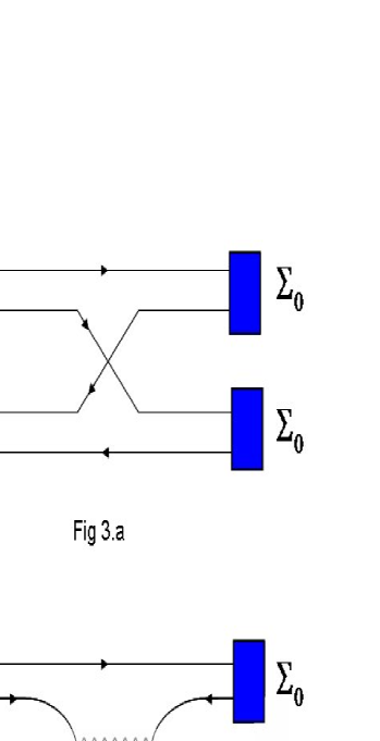
Figure 3: Dominant (3.a) and subdominant (3.b) contributions to the linear terms in the scalar-isoscalar tetraquark fields, which generate a non-zero vacuum expectaion value for the latter, see Eq. (50). At both vertices the the $vev$’s of the scalar-isoscalar quarkonia fields, encoded in the matrix $\Sigma_{0}$ of Eq. (7), appear.

References

- [1] C. Amsler and N. A. Tornqvist, Phys. Rept. 389, 61 (2004).
- [2] F. E. Close and N. A. Tornqvist, J. Phys. G 28, R249 (2002) [arXiv:hep-ph/0204205];
- [3] R. L. Jaffe, Phys. Rept. 409 (2005) 1 [Nucl. Phys. Proc. Suppl. 142 (2005) 343] [arXiv:hep-ph/0409065].
- [4] C. Amsler and F. E. Close, Phys. Lett. B 353, 385 (1995) [arXiv:hep-ph/9505219]; C. Amsler and F. E. Close, Phys. Rev. D 53, 295 (1996) [arXiv:hep-ph/9507326].
- [5] W. J. Lee and D. Weingarten, Phys. Rev. D 61, 014015 (2000) [arXiv:hep-lat/9910008];
- [6] M. Strohmeier-Presicek, T. Gutsche, R. Vinh Mau and A. Faessler, Phys. Rev. D 60, 054010 (1999) [arXiv:hep-ph/9904461].
- [7] F. E. Close and A. Kirk, Eur. Phys. J. C 21, 531 (2001) [arXiv:hep-ph/0103173].
- [8] F. Giacosa, T. Gutsche and A. Faessler, Phys. Rev. C 71, 025202 (2005) [arXiv:hep-ph/0408085].
- [9] F. Giacosa, T. Gutsche, V. E. Lyubovitskij and A. Faessler, Phys. Rev. D 72, 094006 (2005) [arXiv:hep-ph/0509247].
- [10] F. Giacosa, T. Gutsche, V. E. Lyubovitskij and A. Faessler, Phys. Lett. B 622, 277 (2005) [arXiv:hep-ph/0504033].
- [11] H. Y. Cheng, C. K. Chua and K. F. Liu, arXiv:hep-ph/0607206.
- [12] X. G. He, X. Q. Li, X. Liu and X. Q. Zeng, Phys. Rev. D 73 (2006) 114026 [arXiv:hep-ph/0604141]. X. G. He, X. Q. Li, X. Liu and X. Q. Zeng, Phys. Rev. D 73 (2006) 051502 [arXiv:hep-ph/0602075].
- [13] M. B. Voloshin and L. B. Okun, JETP Lett. 23, 333 (1976) [Pisma Zh. Eksp. Teor. Fiz. 23, 369 (1976)]. K. Maltman and N. Isgur, Phys. Rev. Lett. 50, 1827 (1983). K. Maltman and N. Isgur, Phys. Rev. D 29, 952 (1984).
- [14] N. A. Tornqvist, Phys. Rev. Lett. 67, 556 (1991). N. A. Tornqvist, Z. Phys. C 61, 525 (1994) [arXiv:hep-ph/9310247]. T. E. O. Ericson and G. Karl, Phys. Lett. B 309, 426 (1993).
- [15] J. A. Oller, E. Oset and J. R. Pelaez, Phys. Rev. D 59, 074001 (1999) [Erratum-ibid. D 60, 099906 (1999)] [arXiv:hep-ph/9804209].
- [16] R. L. Jaffe, Phys. Rev. D 15 (1977) 267. R. L. Jaffe, Phys. Rev. D 15 (1977) 281. R. L. Jaffe and F. E. Low, Phys. Rev. D 19, 2105 (1979).
- [17] L. Maiani, F. Piccinini, A. D. Polosa and V. Riquer, Phys. Rev. Lett. 93 (2004) 212002 [arXiv:hep-ph/0407017].
- [18] F. Giacosa, Phys. Rev. D 74 (2006) 014028 [arXiv:hep-ph/0605191].
- [19] A. De Rujula, H. Georgi and S. L. Glashow, Phys. Rev. D 12 (1975) 147. T. A. DeGrand, R. L. Jaffe, K. Johnson and J. E. Kiskis, Phys. Rev. D 12 (1975) 2060.
- [20] G. ’t Hooft, Phys. Rev. D 14, 3432 (1976) [Erratum-ibid. D 18, 2199 (1978)].
- [21] E. V. Shuryak, Nucl. Phys. B 203 (1982) 93. T. Schafer and E. V. Shuryak, Rev. Mod. Phys. 70 (1998) 323 [arXiv:hep-ph/9610451]. E. Shuryak and I. Zahed, Phys. Lett. B 589 (2004) 21 [arXiv:hep-ph/0310270].
- [22] U. Vogl and W. Weise, “The Nambu and Jona Lasinio model: Its implications for hadrons and Prog. Part. Nucl. Phys. 27 (1991) 195.
- [23] P. Maris and C. D. Roberts, Int. J. Mod. Phys. E 12 (2003) 297 [arXiv:nucl-th/0301049].
- [24] M. G. Alford and R. L. Jaffe, Nucl. Phys. B 578 (2000) 367 [arXiv:hep-lat/0001023].
- [25] F. Okiharu, H. Suganuma, T. T. Takahashi and T. Doi, arXiv:hep-lat/0601005.
- [26] N. Mathur et al., arXiv:hep-ph/0607110.
- [27] W. M. Yao et al. [Particle Data Group], J. Phys. G 33 (2006) 1.
- [28] E. Van Beveren, T. A. Rijken, K. Metzger, C. Dullemond, G. Rupp and J. E. Ribeiro, Z. Phys. C 30 (1986) 615.
- [29] S. Ishida, M. Ishida, T. Ishida, K. Takamatsu and T. Tsuru, Prog. Theor. Phys. 98 (1997) 621 [arXiv:hep-ph/9705437].
- [30] D. Black, A. H. Fariborz, F. Sannino and J. Schechter, Phys. Rev. D 58 (1998) 054012 [arXiv:hep-ph/9804273].
- [31] D. V. Bugg, Eur. Phys. J. C 47 (2006) 57 [arXiv:hep-ph/0603089].
- [32] D. V. Bugg, Eur. Phys. J. C 47 (2006) 45 [arXiv:hep-ex/0603023].
- [33] D. Black, A. H. Fariborz, S. Moussa, S. Nasri and J. Schechter, Phys. Rev. D 64 (2001) 014031 [arXiv:hep-ph/0012278].
- [34] A. H. Fariborz, R. Jora and J. Schechter, Phys. Rev. D 72 (2005) 034001 [arXiv:hep-ph/0506170]. A. H. Fariborz, Int. J. Mod. Phys. A 19 (2004) 2095 [arXiv:hep-ph/0302133].
- [35] M. Napsuciale and S. Rodriguez, Phys. Rev. D 70 (2004) 094043 [arXiv:hep-ph/0407037].
- [36] A. H. Fariborz, Phys. Rev. D 74 (2006) 054030 [arXiv:hep-ph/0607105].
- [37] S. Gasiorowicz and D. A. Geffen, Rev. Mod. Phys. 41 (1969) 531.
- [38] E. van Beveren, F. Kleefeld, G. Rupp and M. D. Scadron, Mod. Phys. Lett. A 17 (2002) 1673 [arXiv:hep-ph/0204139].
- [39] M. D. Scadron, G. Rupp, F. Kleefeld and E. van Beveren, Phys. Rev. D 69 (2004) 014010 [Erratum-ibid. D 69 (2004) 059901] [arXiv:hep-ph/0309109].
- [40] J. Schaffner-Bielich and J. Randrup, Phys. Rev. C 59 (1999) 3329 [arXiv:nucl-th/9812032]. J. Schaffner-Bielich, Phys. Rev. Lett. 84 (2000) 3261 [arXiv:hep-ph/9906361].
- [41] S. Prelovsek, C. Dawson, T. Izubuchi, K. Orginos and A. Soni, ‘ Phys. Rev. D 70 (2004) 094503 [arXiv:hep-lat/0407037]. T. Burch, C. Gattringer, L. Y. Glozman, C. Hagen, C. B. Lang and A. Schafer, Phys. Rev. D 73 (2006) 094505 [arXiv:hep-lat/0601026].
- [42] C. McNeile and C. Michael [UKQCD Collaboration], Phys. Rev. D 74 (2006) 014508 [arXiv:hep-lat/0604009].
- [43] J. R. Pelaez, Phys. Rev. Lett. 92 (2004) 102001 [arXiv:hep-ph/0309292]. Mod. Phys. Lett. A 19 (2004) 2879 [arXiv:hep-ph/0411107].
- [44] J. R. Pelaez and G. Rios, Phys. Rev. Lett. 97 (2006) 242002 [arXiv:hep-ph/0610397].
- [45] Z. Liu and T. DeGrand, arXiv:hep-lat/0609038.
- [46] D. K. Hong, Y. J. Sohn and I. Zahed, Phys. Lett. B 596 (2004) 191 [arXiv:hep-ph/0403205].
- [47] E. Witten, Nucl. Phys. B 160 (1979) 57.
- [48] E. Klempt, arXiv:hep-ph/0409148.
- [49] E. P. Venugopal and B. R. Holstein, Phys. Rev. D 57, 4397 (1998) [arXiv:hep-ph/9710382].
- [50] V. Baru, J. Haidenbauer, C. Hanhart, A. Kudryavtsev and U. G. Meissner, Eur. Phys. J. A 23 (2005) 523 [arXiv:nucl-th/0410099].
- [51] C. A. Baker et al., Phys. Lett. B 563, 140 (2003).
- [52] C. Morningstar and M. J. Peardon, AIP Conf. Proc. 688 (2004) 220 [arXiv:nucl-th/0309068].
- [53] K. Peters, Int. J. Mod. Phys. A 20 (2005) 570.
- [54] D. Morgan and M. R. Pennington, Phys. Rev. D 48 (1993) 1185. N. N. Achasov and V. N. Ivanchenko, Nucl. Phys. B 315 (1989) 465. N. N. Achasov, arXiv:hep-ph/0410051.
- [55] Y. Kalashnikova, A. Kudryavtsev, A. V. Nefediev, J. Haidenbauer and C. Hanhart, Phys. Rev. C 73 (2006) 045203 [arXiv:nucl-th/0512028].
- [56] F. Giacosa, T. Gutsche, V. E. Lyubovitskij and A. Faessler, Phys. Rev. D 72 (2005) 114021 [arXiv:hep-ph/0511171].