CP-odd static electromagnetic properties of the $W$ gauge boson and the $t$ quark via the anomalous $tbW$ coupling

Abstract

In the framework of the electroweak chiral Lagrangian, the one-loop induced effects of the anomalous $tbW$ coupling, which includes both left- and right-handed complex components, on the static electromagnetic properties of the $W$ boson and the $t$ quark are studied. The attention is focused mainly on the CP-violating electromagnetic properties. It is found that the $tbW$ anomalous coupling can induce both CP-violating moments of the $W$ boson, namely, its electric dipole ($\widetilde{\mu}_{W}$) and magnetic quadrupole ($\widetilde{Q}_{W}$) moments. As far as the $t$ quark is concerned, a potentially large electric dipole moment $(d_{t})$ can arise due to the anomalous $tbW$ coupling. The most recent bounds on the left- and right-handed parameters from $B$ meson physics lead to the following estimates $\widetilde{\mu}_{W}\sim 4\times 10^{-23}-4\times 10^{-22}$ e$\cdot$ cm and $\widetilde{Q}_{W}\sim 10^{-38}-10^{-37}$ e$\cdot$ cm², which are $7$ and $14$ orders of magnitude larger than the standard model (SM) predictions, whereas $d_{t}$ may be as large as $10^{-22}$ e$\cdot$cm, which is about $8$ orders of magnitude larger than its SM counterpart.

I Introduction

The only source of CP violation in the standard model (SM) is the Cabbibo-Kobayashi-Maskawa (CKM) phase, which seems to be the origin of CP violation in nondiagonal processes CKMND , as suggested by the experimental data on $B$-$\bar{B}$ mixing BBM . Several studies DS suggest, however, that the CKM phase has a rather marginal effect on CP-violating flavor-diagonal processes such as the electric dipole moments (EDM) of elementary particles, which means that this class of properties may be highly sensitive to any new physics effects. While the static electromagnetic properties of the leptons have been long studied both theoretically and experimentally, those of the heaviest SM particles still require more attention. In particular, the CP-violating properties of the $W$ boson and the top quark are extremely suppressed in the SM (the $W$ boson EDM arises up to two loops and the top quark EDM arises first at three loops), so their study may shed light on the origin of CP violation. It is thus worth analyzing alternative sources of CP violation that may manifest themselves via the static electromagnetic properties of the $W$ boson and the top quark.

The fact that the on-shell $WW\gamma$ vertex is gauge-independent has long motivated the study of its behavior under radiative corrections because this allows one to estimate the sensitivity of the Yang-Mills sector to any physics beyond the Fermi scale. Much theoretical work has gone into studying the CP-even static electromagnetic properties of the $W$ boson, but its experimental determination still awaits a higher experimental precision. As far as the CP-odd electromagnetic properties are concerned, they are by far more suppressed within the SM, thereby offering an ideal laboratory for searching for any new physics effects. By invoking Lorentz and electromagnetic gauge invariance, regardless of $C$, $P$, or $T$ conservation, the on-shell $WW\gamma$ vertex can be characterized by five independent form factors FF . Three of these form factors are CP-even $(g_{1},\kappa,\Delta Q)$ and two are CP-odd, $(\widetilde{\kappa},\widetilde{Q})$. While $g_{1}$ and $\kappa$ are already generated at the level of the classical action, $\Delta Q$ first arises at the one-loop level. The anomalous contributions to $\kappa$ and $\Delta Q$ have been calculated in the SM WWgSM and several of its extensions WWgNP . As for the CP-odd form factors, they are naturally suppressed because they can only arise at the one-loop level or higher orders in any renormalizable theory. Despite their suppression, the scrutiny of the CP-violating $W$ boson properties may provide relevant information for our knowledge of CP violation. The electric dipole and magnetic quadrupole moments can be generated at the one-loop level via the $\widetilde{\kappa}$ form factor in some extended models. Since the presence of a trace involving the $\gamma_{5}$ Dirac matrix is necessary in order to generate a Levi-Civitta tensor, it is clear that these CP-violating moments can only be induced at the one-loop level via a fermionic loop. It has been shown that this class of effects can arise in theories including both left- and right-handed fermion currents with a complex phase Burgess ; TT1 . This possibility has already been explored within the context of left-right symmetric models Burgess , though the respective contribution was found highly suppressed due to the experimental constraints on the $W_{L}-W_{R}$ mixing.

As far as the static electromagnetic properties of the top quark are concerned, the forthcoming years will see a vigorous boost in the theoretical interest and experimental scrutiny of this particle’s properties. Specifically, the largest priority at the CERN large hadron collider (LHC) is the study of the top quark fundamental properties, and further studies are planned at the next linear collider (NLC) via top quark pair production. Interesting experimental and theoretical prospects are open due to the fact that the top quark has a mass of the order of the Fermi scale, which poses the question whether it is just an ordinary quark or a composite particle. The top quark decays very quickly, mainly into a $bW$ pair, before any hadronization takes place, which may allow one to examine its properties without the presence of any unwanted QCD effects, which invariably would swamp the processes involving the light quarks. This peculiarity opens the door to the scrutiny of the top quark electromagnetic properties, thereby allowing the possibility of detecting a nonvanishing CP-violating electric dipole moment (EDM). Several studies have been devoted to analyze the electric or weak dipole form factors of the top quark and the so induced CP violation. Along these lines, several studies on CP violation in $\bar{t}t$ production have been pursued in the context of hadron HC , $e^{+}e^{-}$ EPC , and $\gamma\gamma$ PPC colliders. Despite its suppression in the SM, the top quark EDM can be significantly enhanced in a broad class of beyond-the-SM extensions. For instance, studies within the context of multi-Higgs models EDMMH have shown that the top quark EDM may be several orders of magnitude larger than the SM prediction.

Since the study of the CP-odd static electromagnetic properties of the $W$ boson and the top quark may hint to the origin of CP violation, it is worth considering any possible sources of this class of effects. In this work, we are interested in the potential CP-violating effects of the most general dimension-four $tbW$ coupling, which involves both left- and right-handed components with a complex phase, on the CP-odd static electromagnetic properties of the $W$ boson and the top quark. The relevance of this coupling is evident from the fact that the top quark decays mainly into a $bW$ pair. Although there is a plenty of theoretical work that has considered its tree-level effects, it is also interesting to study its possible impact in one-loop processes. Due to the large mass of the top quark, which is the only known quark with a mass of the order of the electroweak scale, it has been conjectured that it may induce new dynamics effects and even more play a special role in the mechanism of mass generation, which has attracted the interest on the study of any anomalous contributions to its couplings to other SM particles. Even more, the copious production of top quark events expected at the LHC will allow us to study more carefully the top quark properties and examine possible new physics effects induced by this particle. Very interestingly, this class of new physics effects would arise at the electroweak scale, in contrast with other type of new physics efffects that are expected to arise at heavier energy scales.

The role that the $tbW$ coupling might play in a scenario in which the mass is not generated via the Higgs mechanism has been examined by several authors tbW through diverse phenomenological studies EWCL ; Peccei:1989kr . Instead of considering a specific model, we will adopt a model-independent approach by considering the $tbW$ anomalous contributions in the context of an electroweak chiral Lagrangian (EWCL) EWCL in which the $SU_{L}(2)\times U_{Y}(1)$ symmetry is nonlinearly realized as it is assumed that the Higgs boson is very heavy or does not exist at all. We can think of this scenario as the one in which the EWCL parametrizes unknown physics that is not dictated by the Higgs mechanism. Several authors have already studied this vertex in this context, and diverse scenarios have been taken into account to obtain limits on the left- and right-handed couplings LIMPHASES1 ; LIMPHASES2 ; LIMEWO ; LIMUNITARITY . Along these lines, some top quark production mechanisms have been considered PRODUCTION . In particular, some hadronic processes have been used to impose limits on the CP-violating phases associated with the general left- and right-handed structure of the $tbW$ coupling LIMPHASES1 ; LIMPHASES2 . These results will be used below to estimate the values of the $W$ electric dipole and magnetic quadrupole moments. Thus, the main aim of this work is using the most recent bounds on the anomalous terms of the $tbW$ vertex to predict the effects of this coupling on the static electromagnetic properties of the $W$ boson and the top quark. This approach is in accordance with the spirit of the effective Lagrangian approach.

This paper has been organized as follows. The most general structure of the $tbW$ vertex is introduced in the context of the EWCL in Sec. II, whereas the respective contribution to the CP-violating static electromagnetic properties of the $W$ boson and the top quark are calculated in Sec. III. Section IV is devoted to analyze our results, and the conclusions are presented in Sec. V.

II Theoretical framework

If the Higgs mechanism is not realized in nature, whatever is the true mechanism responsible for the electroweak symmetry breaking, it would open unexpected avenues for new physics effects. In particular, new sources of CP violation might show up. The unknown new physics can be parametrized using the effective Lagrangian technique in which the electroweak symmetry is nonlinearly realized. The resultant Lagrangian is known as the EWCL. In this approach, the Higgs doublet is replaced by a dimensionless matrix field that transforms nonlinearly under the $SU_{L}(2)\times U_{Y}(1)$ group tbW ; EWCL :

$$\Sigma=\exp\Big{(}\frac{i\phi^{a}\sigma^{a}}{v}\Big{)},$$ (1)

where $\phi^{a}$ ($a=1,2,3$) are Goldstone bosons, $\sigma^{a}$ are the Pauli matrices, and $v$ is the Fermi scale. Under the $SU_{L}(2)\times U_{Y}(1)$ group, $\Sigma$ transform as:

$$\Sigma^{\prime}=L\Sigma R^{\dagger},$$ (2)

where

$$L = \exp\Big{(}\frac{i\alpha^{a}\sigma^{a}}{2}\Big{)},$$ (3)

$$R = \exp\Big{(}\frac{i\beta\sigma^{3}}{2}\Big{)},$$ (4)

with $\alpha^{a}$ and $\beta$ being the parameters of the $SU_{L}(2)$ and $U_{Y}(1)$ groups, respectively. From these expressions, it is easy to see that the Goldstone bosons fields transform nonlinearly under the electroweak group. In this scheme, the gauge fields are defined in the following way

$$\hat{W}_{\mu} = \frac{\sigma^{a}W^{a}_{\mu}}{2i},$$ (5)

$$\hat{B}_{\mu} = \frac{\sigma^{3}B_{\mu}}{2i}.$$ (6)

To define the most general expression for the charged current, it is necessary to introduce some bosonic and fermionic Lorentz structures. We need the following Lorentz tensors:

$$\Sigma^{a}_{\mu} = -\frac{i}{2}Tr[\sigma^{a}\Sigma^{\dagger}D_{\mu}\Sigma],$$ (7)

$$\Sigma^{a}_{\mu\nu} = -iTr[\sigma^{a}\Sigma^{\dagger}[D_{\mu},D_{\nu}]\Sigma],$$ (8)

where

$$D_{\mu}\Sigma=\partial_{\mu}\Sigma-g\hat{W}_{\mu}\Sigma+g^{\prime}\Sigma\hat{B}_{\mu}.$$ (9)

The charged fields are given by the following relations

$$\Sigma^{\pm}_{\mu} = \frac{1}{\sqrt{2}}(\Sigma^{1}_{\mu}\mp i\Sigma^{2}_{\mu}),$$ (10)

$$\Sigma^{\pm}_{\mu\nu} = \frac{1}{\sqrt{2}}(\Sigma^{1}_{\mu\nu}\mp i\Sigma^{2}_{\mu\nu}).$$ (11)

In the unitary gauge ($\phi^{a}=0$), these expressions become $\Sigma^{\pm}_{\mu}=g/2\,W^{\pm}_{\mu}$ and

$$\Sigma^{\pm}_{\mu\nu}=g[W^{\pm}_{\mu\nu}\pm ie(W^{\pm}_{\mu}A_{\nu}-W^{\pm}_{\nu}A_{\mu})\pm igc_{W}(W^{\pm}_{\mu}Z_{\nu}-W^{\pm}_{\nu}Z_{\mu})],$$ (12)

where $c_{W}$ stands for $\cos\theta_{W}$. We also need the following fermion operators:

$$\Delta_{L} = \bar{t}P_{L}b,\ \ \ \Delta^{\mu}_{L}=\bar{t}\gamma^{\mu}P_{L}b,$$ (13)

$$\Delta_{R} = \bar{t}P_{R}b,\ \ \ \Delta^{\mu}_{R}=\bar{t}\gamma^{\mu}P_{R}b,$$ (14)

$$\Delta^{\mu\nu}_{L} = \bar{t}\sigma^{\mu\nu}P_{L}b,\ \ \ \bar{\Delta}^{\mu}_{L}=i\bar{t}P_{L}\bar{D}^{\mu}b,$$ (15)

$$\Delta^{\mu\nu}_{R} = \bar{t}\sigma^{\mu\nu}P_{R}b,\ \ \ \bar{\Delta}^{\mu}_{R}=i\bar{t}P_{R}\bar{D}^{\mu}b,$$ (16)

where $\bar{D}_{\mu}=\partial_{\mu}-ieQA_{\mu}$ is the electromagnetic covariant derivative, $\sigma_{\mu\nu}=(i/2)[\gamma_{\mu},\gamma_{\nu}]$, and $P_{L}(P_{R})$ is the left-handed(right-handed) projector.

Using the above expressions, the most general Lagrangian for the charged currents can be written as

$${\cal L}^{CC} = \sqrt{2}a_{L}\Delta^{\mu}_{L}\Sigma^{+}_{\mu}+\sqrt{2}a_{R}\Delta^{\mu}_{R}\Sigma^{+}_{\mu}+\frac{1}{\Lambda}\Big{[}ib_{L}\Delta_{L}\bar{D}^{\mu}\Sigma^{+}_{\mu}+ib_{R}\Delta_{R}\bar{D}^{\mu}\Sigma^{+}_{\mu}$$ (17)

$$+c_{L}\bar{\Delta}^{\mu}_{L}\Sigma^{+}_{\mu}+c_{R}\bar{\Delta}^{\mu}_{R}\Sigma^{+}_{\mu}+d_{L}\Delta^{\mu\nu}_{L}\Sigma^{+}_{\mu\nu}+d_{R}\Delta^{\mu\nu}_{R}\Sigma^{+}_{\mu\nu}\Big{]}+{\rm H.c.},$$

with $\Lambda$ being an energy scale. We have introduced the $\sqrt{2}$ factor in order to recover the SM value ($g/\sqrt{2}$) for the left-handed coupling in the appropriate limit. Although this Lagrangian induces the vertices $tbW$, $tbW\gamma$ and $tbWZ$, we only show the first one:

$${\cal L}_{tbW} = \frac{g}{2}\Big{\{}\sqrt{2}\bar{t}(a_{L}P_{L}+a_{R}P_{R})bW^{+}_{\mu}+\frac{1}{\Lambda}\Big{[}i\bar{t}(b_{L}P_{L}+b_{R}P_{R})b\partial^{\mu}W^{+}_{\mu}$$ (18)

$$+i\bar{t}(c_{L}P_{L}+c_{R}P_{R})\partial^{\mu}bW^{+}_{\mu}+2\bar{t}\sigma^{\mu\nu}(d_{L}P_{L}+d_{R}P_{R})bW^{+}_{\mu\nu}\Big{]}\Big{\}}+{\rm H.c.}$$

We will only consider the renormalizable part of this coupling as it is expected to give the dominant contribution to the $WW\gamma$ and $tt\gamma$ vertices. Therefore, all terms proportional to $1/\Lambda$ will be neglected from now on.

A word of caution is in order here. Although we have presented an specific theoretical framework for the presence of an anomalous $tbW$ coupling, our calculation below remains valid for any class of theory predicting an interaction as the one given in Eq. (18). In this context, our results are meant to examine the impact of the anomalous $tbW$ coupling on the static properties of the $W$ boson and the top quark, but they are not mean to test the EWCL scenario. This is beyond the reach of the present work.

III CP-odd static electromagnetic properties of the $W$ boson and the top quark

We now present the explicit calculation of the anomalous $tbW$ coupling to the CP-odd static electromagnetic properties of the $W$ boson and the top quark.

III.1 The $W$ boson EDM and MQM

We now turn to discuss the structure of the $WW\gamma$ vertex and the contribution from the anomalous $tbW$ coupling. The most general on-shell $W_{\alpha}(p-q)W_{\beta}(-p-q)A_{\mu}(2q)$ vertex can be written as

$$\Gamma_{\alpha\beta\mu} = i\,e\bigg{(}g_{1}\left[2\,p^{\mu}g^{\alpha\beta}+4\,(q_{\beta}g_{\alpha\mu}-q_{\alpha}g_{\beta\mu})\right]+2\Delta\kappa(q_{\beta}g_{\alpha\mu}-q_{\alpha}g_{\beta\mu})+\frac{4\,\Delta Q}{m^{2}_{W}}\,p_{\mu}q_{\alpha}q_{\beta}$$ (19)

$$+ 2\widetilde{\kappa}\,\epsilon_{\alpha\beta\mu\lambda}q^{\lambda}+\frac{4\,\widetilde{Q}}{m^{2}_{W}}\,q_{\beta}\epsilon_{\alpha\mu\lambda\rho}p^{\lambda}q^{\rho}\bigg{)},$$

where all the momenta are incoming. In a renormalizable theory, the form factors $\Delta\kappa$, $\Delta Q$, $\widetilde{\kappa}$, and $\widetilde{Q}$ always arise via radiative corrections. The magnetic (electric) dipole moment $\mu_{W}$ ($\widetilde{\mu}_{W}$) and the electric (magnetic) quadrupole moment $Q_{W}$ ($\widetilde{Q}_{W}$) are given in terms of the electromagnetic form factors as follows

$$\mu_{W} = \frac{e}{2\,m_{W}}(2+\Delta\kappa),$$ (20)

$$Q_{W} = -\frac{e}{m^{2}_{W}}(1+\Delta\kappa+\Delta Q),$$ (21)

$$\widetilde{\mu}_{W} = \frac{e}{2\,m_{W}}\widetilde{\kappa},$$ (22)

$$\widetilde{Q}_{W} = -\frac{e}{m^{2}_{W}}(\widetilde{\kappa}+\widetilde{Q}).$$ (23)

The contribution of the $tbW$ coupling arises from the triangle diagrams shown in Fig. 1. We will concentrate only on the CP-odd contribution, although there are also contributions to the CP-even form factors. As already mentioned, at this order of perturbation theory, the renormalizable part of the $tbW$ coupling can only contribute to one CP-odd form factor, namely, $\widetilde{\kappa}$, which reads

$$\widetilde{\kappa}=\frac{\alpha}{8s_{W}^{2}\pi^{2}}\left(Q_{t}F(x_{t},x_{b})+Q_{b}F(x_{b},x_{t})\right)Im\left(a_{L}a_{R}^{\dagger}\right),$$ (24)

where $x_{a}=m_{a}/m_{W}$ and

$$F(x,y)=4\,x\,y\left(\log\left(\frac{x}{y}\right)+\left(1-x^{2}+y^{2}\right)\frac{f(x,y)}{2\chi(x,y)}\right),$$ (25)

with

$$f(x,y)=\log\left(\frac{1-(x^{2}+y^{2})-\delta(x,y)}{1-(x^{2}+y^{2})+\delta(x,y)}\right),$$ (26)

and $\chi^{2}(x,y)=(x^{2}+y^{2}-1)^{2}-4x^{2}y^{2}$. This result is free of ultraviolet divergences, which is a consequence of the fact that only the renormalizable part of the $tbW$ vertex has been considered.

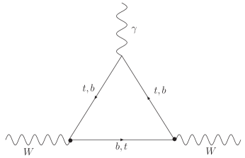
Figure 1: Feynman diagrams contributing to the on-shell $WW\gamma$ vertex. The dot denotes an anomalous $tbW$ vertex.

III.2 The top quark EDM

The most general $tt\gamma$ vertex function is given by

$$\Gamma_{\mu}=i\,\bar{t}(p_{1})\left(\gamma^{\mu}F_{t}+i\sigma^{\mu\nu}q_{\nu}\left(a_{t}+\gamma^{5}d_{t}\right)\right)t(p_{2}),$$ (27)

where $F_{t}$ is the electric charge of the top quark, $a_{t}$ is its MDM, and $d_{t}$ is its EDM. At tree level $Ft=2/3e$, whereas $a_{t}$ and $d_{t}$ arise via radiative corrections.

The anomalous $tbW$ coupling of Eq. (18) induces an EDM for the top quark through the Feynman diagrams shown in Fig. 2, where all the particles are taken on-shell. After some calculation via the unitary gauge, one can extract the coefficient of the $i\gamma^{5}\sigma_{\mu\nu}q^{\nu}$ term from the $\bar{t}t\gamma$ vertex function. Here $q_{\mu}$ is the photon four momentum. This leads to

$$d_{t}=\frac{N_{c}\,\alpha}{32\pi}\,\frac{m_{b}}{m_{W}}\frac{e}{m_{W}}\,\left(Q_{W}F_{W}(x_{b},x_{W})+Q_{b}\,F_{b}(x_{b},x_{W})\right)\,Im\left(a_{L}a_{R}^{*}\right),$$ (28)

with $x_{i}=m_{i}/m_{t}$, $N_{c}=3$, $Q_{b}=-1/3$, and $Q_{W}=-1$. The $F_{W}$ and $F_{b}$ functions stand for the contribution of the Feynman diagram where the photon emerges from the $W$ boson and the $b$ quark line, respectively. They are given by

$$F_{W}(x_{b},x_{W})=\left(x_{b}^{2}-4x_{W}^{2}-1\right)f_{1}(x_{b},x_{W})-\left(x_{b}^{4}+4x_{W}^{4}-5x_{b}^{2}x_{W}^{2}-3x_{W}^{2}-2x_{b}^{2}+1\right)f_{2}(x_{b},x_{W}),$$ (29)

$$F_{b}(x_{b},x_{W})=\left(x_{b}^{2}-4x_{W}^{2}-1\right)f_{1}(x_{W},x_{b})+\left(x_{b}^{4}+4x_{W}^{4}-5x_{b}^{2}x_{W}^{2}-3x_{W}^{2}-2x_{b}^{2}+1\right)f_{2}(x_{W},x_{b}),$$ (30)

with

$$f_{1}(x,y) = 2+\left(1-y^{2}+x^{2}\right)\log\left(\frac{y}{x}\right)+\sqrt{(1-x^{2}-y^{2})^{2}-4x^{2}y^{2}}\,{\rm sech}^{-1}\left(\frac{2xy}{x^{2}+y^{2}-1}\right),$$ (31)

$$f_{2}(x,y) = -\log\left(\frac{y}{x}\right)-\frac{1+x^{2}-y^{2}}{\sqrt{(1-x^{2}-y^{2})^{2}-4x^{2}y^{2}}}\,{\rm sech}^{-1}\left(\frac{2xy}{x^{2}+y^{2}-1}\right).$$

For the same reason argued when discussing the $W$ boson EDM, the calculated top quark EDM is free of ultraviolet divergences.

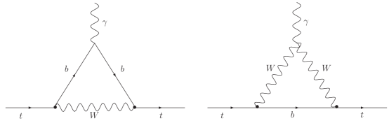
Figure 2: Feynman diagrams contributing to the on–shell $\bar{t}t\gamma$ vertex.

IV Results and discussion

We turn to discuss the numerical results. First of all, we will discuss the most recent bounds on the anomalous $tbW$ coupling from $B$ meson physics. Secondly, we will consider these bounds to predict the order of magnitude expected for the $W$ boson and the top quark EDMs. We would like to emphasize that our main purpose is to obtain a prediction for the $tbW$ effects on the CP-violating static electromagnetic properties of the $W$ boson and the top quark, rather than using our calculation to obtain a bound for the anomalous $tbW$ coupling, for which we could use the neutron EDM for instance. However, a careful study of the effects of the one-loop induced $W$ boson EDM on the nucleon EDM would require a two-loop calculation, which is beyond the purpose of this work. It is worth to discuss this point with more extent. In Ref. MQ , an effective vertex parametrizing the EDM of the $W$ boson was used to calculate a one-loop induced fermion EDM. Somewhat erroneously, we may want follow the same approach here and use the calculation of Ref. MQ to obtain a bound on the $tbW$ anomalous coupling. This could be done safely if the fermions circulating in the loop were much heavier than the external $W$ boson, in which case the one-loop $WW\gamma$ vertex of Fig. 1 could be parametrized as an effective tree-level vertex an inserted into the one-loop $\bar{f}f\gamma$ vertex to calculate the fermion EDM [see Fig. 3 (b)]. Such an approximation is not valid when the $WW\gamma$ loop includes fermions with a mass of the same order of magnitude than the $W$ boson mass, as occurs with the contribution of the $tbW$ vertex. In such a case, the two-loop diagram of Fig. 3 (a) must be evaluated.

Figure 3: Feynman diagrams contributing to the EDM of a fermion via the $W$ EDM when (a)the fermions circulating in the $WW\gamma$ loop have a mass of the same order of magnitude than the $W$ boson mass and (b)the internal fermions are much heavier than the $W$ boson, in which case an effective $WW\gamma$ vertex can be used.

Although there are prospects for the direct measurement of the $tbW$ coupling at the LHC and the planned future colliders, it has been pointed out in Ref. CP that CLEO data on $b\to s\gamma$ are already more constraining on the right-handed $tbW$ coupling than what would be achievable at any planned future collider. Thus, the bounds discussed below will be very useful to assess the impact of this vertex on the $WW\gamma$ and $tt\gamma$ vertices.

IV.1 Bounds on the anomalous $tbW$ coupling

It is customary to parametrize the left- and right-handed parameters of Eq. (18) in the following way

$$a_{L} = 1+\kappa_{L}e^{i\phi_{L}},$$ (32)

$$a_{R} = \kappa_{R}e^{i\phi_{R}},$$ (33)

with $\kappa_{L,R}$ and $\phi_{L,R}$ real parameters. It follows that

$$Im(a_{L}a^{\dagger}_{R})=-\kappa_{R}\sin\phi_{R}+\kappa_{L}\kappa_{R}\sin(\phi_{L}-\phi_{R}).$$ (34)

In the above expressions, the SM left-handed coupling was explicitly introduced along with a deviation characterized by the $\kappa_{L}$ and $\phi_{L}$ parameters. In order to make predictions, we need to assume some values for these parameters. For this purpose, we will consider the bounds reported in the literature, such as the ones obtained in Ref. LIMPHASES1 from $B$ decay processes:

$$\kappa_{L}\sin\phi_{L} < 3\times 10^{-2},$$ (35)

$$\kappa_{R}\sin\phi_{R} < 10^{-3}.$$ (36)

There are also limits on the right-handed parameters derived from the CLEO Collaboration data on the $b\to s\gamma$ decay LIMPHASES2 :

$$\kappa_{R}\cos\phi_{R} < 4\times 10^{-3},$$ (37)

$$\kappa_{R}\sin\phi_{R} < 10^{-3}.$$ (38)

In addition, current data on CP-conserving process allows $\kappa_{L}$ to be as large as $0.2$ CP ; LIMEWO ; LIMUNITARITY . As far as the $\kappa_{R}$ parameter is concerned, it seems to be more suppressed than the corresponding left-handed one, as suggested by Eq. (37) and also from the result obtained in Ref. Yamada , where it was found that $-5\times 10^{-2}<\kappa_{R}<10^{-2}$.

In the following, we will estimate the EDM of the $W$ boson and the top quark using the following values: $\kappa_{L}\sin\phi_{L}<3\times 10^{-2}$, $\kappa_{R}\sin\phi_{R}<10^{-3}$, and $\kappa_{R}<4\times 10^{-3}$.

V The EDM of the $W$ boson

In the context of renormalizable theories with the simultaneous presence of left- and right-handed fermion currents, the electric dipole and magnetic quadrupole moments are proportional at the one-loop level:

$$\widetilde{Q}_{W}=-\Big{(}\frac{2}{m_{W}}\Big{)}\widetilde{\mu}_{W}.$$ (39)

This means that $\widetilde{Q}_{W}$ is suppressed with respect to $\widetilde{\mu}_{W}$ by a factor of the order of $10^{-16}$, provided that units of e and cm are used. However, this hierarchy might not hold at higher orders. Using the known values for the SM parameters, the electric dipole and magnetic quadrupole moments of the $W$ boson can be written as

$$\widetilde{\mu}_{W} = -4\times 10^{-19}Im(a_{L}a^{\dagger}_{R})\quad{\rm e}\cdot{\rm cm},$$ (40)

$$\widetilde{Q}_{W} = 1.98\times 10^{-34}Im(a_{L}a^{\dagger}_{R})\quad{\rm e}\cdot{\rm cm}^{2}.$$ (41)

The constraints of Eqs. (35) and (37) pose two scenarios of interest, for which we get an estimate for the $W$ electric dipole and magnetic quadrupole moments:

• SM-like $a_{L}$ and complex $a_{R}$:

  $$\widetilde{\mu}_{W} = 4\times 10^{-19}\kappa_{R}\sin\phi_{R}\ {\rm e}\cdot{\rm cm}<4\times 10^{-22}\ {\rm e}\cdot{\rm cm},$$ (42)

  $$\widetilde{Q}_{W} = -1.98\times 10^{-34}\kappa_{R}\sin\phi_{R}\ {\rm e}\cdot{\rm cm}^{2}<-1.98\times 10^{-37}\ {\rm e}\cdot{\rm cm}^{2}.$$ (43)

• Complex $a_{L}$ and purely real $a_{R}$:

  $$\widetilde{\mu}_{W} = -4\times 10^{-19}\kappa_{R}\kappa_{L}\sin\phi_{L}\ {\rm e}\cdot{\rm cm}<-4.8\times 10^{-23}\ {\rm e}\cdot{\rm cm},$$ (44)

  $$\widetilde{Q}_{W} = 1.98\times 10^{-34}\kappa_{R}\kappa_{L}\sin\phi_{L}\ {\rm e}\cdot{\rm cm}^{2}<2.38\times 10^{-38}\ {\rm e}\cdot{\rm cm}^{2}.$$ (45)

In the most general scenario, both $a_{L}$ and $a_{R}$ are complex, but the values for $\widetilde{\mu}_{W}$ and $\widetilde{Q}_{W}$ are similar to those obtained in the first scenario above.

It is worth comparing our results with those previously reported in the literature. Of course the standard to which all results should be compared with is the SM prediction. As already mentioned, in the SM $\widetilde{Q}_{W}$ first arises at the two-loop level, whereas $\widetilde{\mu}_{W}$ appears up to three-loop order. It has been estimated that $\widetilde{\mu}_{W}$ and $\widetilde{Q}_{W}$ are of the order of $10^{-29}$ e$\cdot$ cm SMED ; SMED2 and $-10^{-51}$ e$\cdot$ cm² SMMQ , respectively. Beyond the SM, most of the studies have focused on $\widetilde{\mu}_{W}$, with the exception of Ref. TT2 , in which both $\widetilde{\mu}_{W}$ and $\widetilde{Q}_{W}$ were estimated. In sharp contrast with the negligibly small SM predictions, some of its extensions predict values several orders of magnitude larger. For instance, a value of $10^{-22}$ e$\cdot$cm for $\widetilde{\mu}_{W}$ was estimated in left-right symmetric models SMED ; Burgess , and a similar result was found in supersymmetric models, which induce this moment via one-loop diagrams mediated by charginos and neutralinos SMED ; SSM . The $\widetilde{\mu}_{W}$ moment has also been estimated in multi-Higgs models, in which it can be induced at the two-loop level. For instance it was found that $\widetilde{\mu}_{W}\sim 10^{-20}-10^{-21}$ e$\cdot$ cm in the two-Higgs doublet model THDM . A similar value was found in the context of the so-called 331 models, whose Higgs sector also induces $\widetilde{\mu}_{W}$ at the two-loop level 331 . From these results, we can conclude that our estimate for $\widetilde{\mu}_{W}$ in the context of the EWCL lies within the range of the predictions obtained from other renormalizable SM extensions.

It is interesting to mention that the CP-odd static electromagnetic properties of the $W$ boson have been estimated in Ref. TT2 within the context of the linear electroweak effective Lagrangian (LEWEL), which do assume the existence of the Higgs boson, in contrast with the EWCL. It was shown that the most general $HWW$ coupling, which includes both CP-even and CP-odd components, can give rise to both CP-odd $WW\gamma$ form factors $\tilde{\kappa}$ and $\tilde{Q}$. The numerical estimates obtained for appropriate values of the unknown parameters are $\widetilde{\mu}_{W}\sim 3-6\times 10^{-20}$ e$\cdot$ cm and $\widetilde{Q}_{W}\sim-10^{-36}$ e$\cdot$ cm² TT2 . We thus can conclude that the values for $\widetilde{\mu}_{W}$ and $\widetilde{Q}_{W}$ induced by the anomalous $tbW$ coupling, which are about 7 and 17 orders of magnitude above their respective SM predictions, are one order of magnitude smaller that those generated by an anomalous $HWW$ coupling.

V.1 The top quark EDM

Once Eq. (28) is numerically evaluated, one obtains

$$d_{t} = (3.08-5.73)\times 10^{-19}\,Im\left(a_{L}a_{R}^{*}\right)\,{\rm e\cdot cm},$$ (46)

$$= -2.65\times 10^{-19}\,Im\left(a_{L}a_{R}^{*}\right)\,{\rm e\cdot cm},$$

where the positive (negative) contribution corresponds to the the Feynman diagram where the photon emerges from the boson (quark) line. It should be mentioned that $d_{t}$ develops an imaginary part, which is almost twice larger than the real one. The appearance of an imaginary (absortive) part is not usual in the static electromagnetic properties of light particles, but in this case it arises as a consequence of the fact that, being the top quark so heavy, $m_{t}>m_{W}+m_{b}$.

Bearing in mind the constraints of Eqs. (35) and (37), we will explore the two scenarios discussed above. We obtain in the first scenario

$$|d_{t}|\lesssim 2.65\times 10^{-22}\ {\rm e\cdot cm},$$ (47)

whereas the latter scenario leads to

$$|d_{t}|\lesssim 7.95\times 10^{-23}\ {\rm e\cdot cm}.$$ (48)

In this case, the constraint $\kappa_{R}<10^{-2}$ was used.

We also would like to compare our results with those obtained within the framework of other theories. As already mentioned, in the SM the top quark EDM arises first at three loops and it has been estimated to be of the order of $10^{-30}$ e$\cdot$cm SMED ; SMTOPEDM . Beyond the SM, the top quark EDM has also received some attention. For instance, in multi–Higgs models, values for $d_{t}$ lying in the range $10^{-20}-10^{-21}$ e$\cdot$cm have been estimated EDMMH . We can thus conclude that our prediction, which is compatible with the constraints imposed by $B$ meson physics, is about eight orders of magnitude larger than the SM one but one or two orders of magnitude smaller than that obtained in multi–Higgs models.

VI Final remarks

Up to now, the mechanism responsible for electroweak symmetry breaking remains the most puzzling piece of the SM. The Higgs mechanism, although satisfactory to generate the masses of the theory, might be a mere mathematical artifact lacking of any connection with the physical reality. It is therefore important to be open-minded to any potential scenario that may give rise to sizeable new physics effects. Due to its heavy mass, it has been conjectured that the top quark may play a special role in the mass generation. Along these lines, it is worth considering potential new physics effects induced by the top quark. In this paper, we have explored the possible CP-violating effects arising from the most general dimension-four $tbW$ coupling. In particular, the impact of such a coupling on the CP-odd electromagnetic properties of the $W$ boson and the top quark was studied. Analytical expressions were obtained, and their numerical values were estimated by considering the most recent bounds on the $tbW$ coupling phases from $B$ meson physics, as reported in the literature.

It was found that the most promising scenario corresponds to an anomalous $tbW$ coupling with a SM-like left-handed part and a complex right-handed component. In such a scenario, the resultant predictions for the $W$ CP-odd static electromagnetic properties are $\widetilde{\mu}_{W}<4\times 10^{-22}$ e$\cdot$ cm and $\widetilde{Q}_{W}<1.98\times 10^{-37}$ e$\cdot$ cm², which are 7 and 14 orders of magnitude larger than the respective SM prediction, whereas the top quark EDM $d_{t}$ may be up to eight orders of magnitude larger than the SM contribution. Another interesting scenario corresponds to an anomalous $tbW$ coupling with a complex left-handed component and a purely real right-handed component, but in such a case the static properties of the $W$ boson and the top quark are one order of magnitude smaller than in the precious scenario. We have also compared our results with those obtained in the framework of other beyond-the-SM theories. It was found that our results are about one order of magnitude smaller than those predicted by other theories such as multi-Higgs doublet models. Since an anomalous $tbW$ coupling can arise in a scenario where the Higgs boson is absent, it is interesting to compare our results with those obtained in theories where the Higgs boson is the one responsible for the electroweak symmetry breaking. For instance, in Ref. TT2 a general $HWW$ coupling involving both CP-even and CP-odd components was considered, which gives rise to both $\widetilde{\mu}_{W}$ and $\widetilde{Q}_{W}$. Our results, obtained in the Higgsless EWCL scenario, are about one order of magnitude smaller than those induced in the scenario where at least one relatively light Higgs boson is present.

The EDM of the $W$ boson can contribute significantly to the EDM of light fermions, such as the electron and the neutron, which are under frequent experimental scrutiny. This fact was exploited by the authors of Ref. MQ , in which the experimental upper bound on the neutron electric dipole moment, $d_{n}<10^{-25}$ e$\cdot$ cm, was used to obtain the upper bound $\widetilde{\mu}_{W}<10^{-20}$ e$\cdot$ cm. Our result for $\widetilde{\mu}_{W}$ is consistent with this result. On the other hand, the direct measurement of the CP-odd structure of the $WW\gamma$ vertex might be in the range of sensitivity of next linear colliders (NLC) or CLIC NLC , which will operate as a $W$ factory. The possibility of extracting some CP-odd asymmetries from these colliders has been examined by several authors, mainly in a model-independent manner via the effective Lagrangian technique AS .

Alternatively, we could use our calculation to obtain bounds on the anomalous $tbW$ coupling from the EDM of the neutron. Although in Ref. MQ an effective $WW\gamma$ vertex was used to calculate the respective contribution to the neutron EDM and the resultant constraint on the CP-odd $WW\gamma$ coupling can be used to constrain the anomalous $tbW$ coupling, a precise estimate would require a two-loop calculation, which is beyond the purpose of this work.

- (1) J. H. Christenson, J. W. Cronin, V. L. Fitch, and R. Turlay, Phys. Rev. Lett. 13, 138 (1964); J. Alexander et al. [Heavy Flavor Averaging Group (HFAG) Collaboration], hep-ex/0412073.
- (2) A. Soni, La Thuile 2005, Results and perspectives in particle physics, 417-441, hep-ph/0509180.
- (3) For a review, see M. Pospelov and A. Ritz, Ann. Phys. (N.Y.) 318, 138 (1964).
- (4) K. J. F. Gaemers and G. J. gounaris, Z. Phys. C1, 259 (1979); K. Hagiwara, R. D. Peccei, D. Zeppenfeld, and K. Hikasa, Nucl. Phys. B282, 253 (1987); F. Boudjema and C. Hamzaoui, Phys. Rev. D43, 3748 (1991).
- (5) W. A. Bardeen, R. Gastmans, and B. Lautrup, Nucl. Phys. B46, 319 (1972); G. Couture, J. N. Ng, Z. Phys. C35, 65 (1987).
- (6) G. Couture, J. N. Ng, J. L. Hewett, and T. G. Rizzo, Phys. Rev. D36, 859 (1987); C. L. Bilachak, R. Gatsmans, and A. van Proeyen, Nucl. Phys. B, 46 (1986); G. Couture, J. N. Ng, J. L. Hewett, and T. G. Rizzo, Phys. Rev. D38, 860 (1988); A. B. Lahanas and V. C. spanos, Phys. Lett. B334, 378 (1994); T. M. Aliyev, ibid. 155, 364 (1985); A. Arhrib, J. L. Kneur, and G. Moultaka, ibid., 376, 127 (1996); N. K. Sharma, P. Saxena, Sardar Singh, A. K. Nagawat, and R. S. Sahu, Phys. Rev. D56, 4152 (1997); T. G. Rizzo and M. A. Samuel, Phys. Rev. D35, 403 (1987); A. J. Davies, G. C. Joshi, and R. R. Volkas, ibid., 42, 3226 (1990); F. Larios, J. A. Leyva, and R. Martínez, Phys. Rev. D53, 6686 (1996); G. Tavares-Velasco and J. J. Toscano, Phys. Rev. D65, 013005 (2001); ibid. 69, 017701 (2004); J. L. García-Luna, G. Tavares-Velasco, and J. J. Toscano, Phys. Rev. D69, 093005 (2004).
- (7) G. Tavares-Velasco and J. J. Toscano, J. Phys. G30, 1299 (2004).
- (8) D. Atwood, C. P. Burgess, C. Hamzaoui, B. Irwin, and J. A. Robinson, Phys. Rev. D42, 3770 (1990).
- (9) J. F. Nieves and P. B. Pal, Phys. Rev. D55, 3118 (1991); G. Tavares-Velasco and J. J. Toscano, Phys. Rev. D70, 053006 (2004).
- (10) C. R. Schimidt and M. E. Peskin, Phys. Rev. Lett. 69, 410 (1992); C. R. Schimidt, Phys. Lett. B293, 111 (1992); A. Brandenburg and J. P. Ma, Z. Phys. C56, 97 (1992); Phys. Lett. B298, 211 (1993); W. Bernreuther and A. Brandenburg, Phys. Rev. D49, 4481 (1994); P. Haberl, O. Nachtmann, and A. Wilch, Phys. Rev. D53, 4875 (1996); B. Grzadkowski and B. Lampe, Phys. Lett. B415, 193 (1997).
- (11) J. F. Donoghue and G. Valencia, Phys. Rev. Lett. 58, 451 (1987); G. L. Kane, G. A. Ladinsky, and C.-P. Yuan, Phys. Rev. D45, 124 (1991); D. Atwood and A. Soni, Phys. Rev. D45, 2405 (1992); W. Bernreuther, O. Nachtmann, P. Overmann, T. Schroder, Nucl. Phys. B388, 53 (1992); B. Grzadkowski, Phys. Lett. B305, 384 (1993); D. Chang, W.-Y. Keung, and I. Phillips, Nucl. Phys. B408, 286 (1993); T. Arens and L. M. Sehgal, Phys. Rev. D50, 4372 (1994); P. Poulose and S. D. Rindani, Phys. Lett. B349, 379 (1995); F. Cuypers and S. Rindani, Phys. Lett. B343, 333 (1995); W. Hollik, J. I. Illana, S. Rigolin, C. Schappacher, and D. Stockinger, Nucl. Phys. B551, 3 (1999).
- (12) S. Y. Choi and K. Hagiwara, Phys. Lett. B359, 369 (1995); H. Anlauf, W. Bernreuther, and A. Brandenburg, Phys. Rev. D52, 3803 (1995); M. S. Baek, S. Y. Choi, and C. S. Kim, Phys. Rev. D56, 6835 (1997); P. Poilose and S. D. Rindani, Phys. Rev. D57, 5444 (1998); Phys. Lett. B452, 347 (1999).
- (13) A. Soni and R. M. Xu, Phys. Rev. Lett. 69, 33 (1992); D. Gómez Dumm and G. A. González-Sprinberg, Eur. Phys. J. C11, 293 (1999); E. O. Iltan, Phys. Rev. D65, 073013 (2002).
- (14) E. Malkawi and C. -P. Yuan, Phys. Rev. D50, 4462 (1994); ibid. 52, 472 (1995); F. Larios and C.-P. Yuan, Phys. Rev. D55, 7218 (1997).
- (15) S. Weinberg, Physica 96A, 327 (1979); S. Coleman, J. Wess, and B. Zumino, Phys. Rev. 177, 2239 (1969); C. G. Callan, S. Coleman, J. Wess, and B. Zumino, ibid. 177, 2247 (1969); H. Georgi, Weak Interactions and Modern Particle Theory (Benjamin/Cummings Menlo Park, CA, 1984).
- (16) R. D. Peccei and X. Zhang, Nucl. Phys. B 337, 269 (1990); R. D. Peccei, S. Peris and X. Zhang, Nucl. Phys. B 349, 305 (1991).
- (17) A. Abd El-Hady and G. Valencia, Phys. Lett. B414, 173 (1997).
- (18) F. Larios, M. A. Pérez, and C.-P. Yuan, Phys. Lett. B457, 334 (1999).
- (19) S. Dawson and G. Valencia, Phys. Rev. D53, 1721 (1996).
- (20) M. Hosch, K. Whisnant, and Bing-Lin Young, Phys. Rev. D55, 3137 (1997).
- (21) S. Dawson and G. Valencia, Phys. Rev. D52, 2717 (1995); F. del Águila and J. A. Aguilar-Saavedra, Phys. Rev. D67, 014009 (2003); S. D. Rindani, Pramana 54, 791 (2000).
- (22) W. J. Marciano and A. Queijeiro, Phys. Rev. D33, 3449 (1986).
- (23) D. Carlson, E. Malkawi, and C. P. Yuan, Phys. Lett. B337, 145 (1994).
- (24) K. Fukikawa and A. Yamada, Phys. Rev. D49, 5859 (1994).
- (25) M. E. Pospelov and I. B. Khriplovich, Sov. J. Nucl. Phys. 53, 638 (1991)[Yad. Fiz.53, 1030 (1991)]; E. P. Shabalin, Sov. J. Nucl. Phys. 28, 75 (1978)[Yad. Fiz. 28, 151 (1978)].
- (26) M. J. Booth, hep-ph/9301293.
- (27) I. B. Khriplovich and M. E. Pospelov, Nucl. Phys. B420, 505 (1994).
- (28) J. Montaño, F. Ramírez-Zavaleta, G. Tavares-Velasco, and J. J. Toscano, Phys. Rev. D72, 115009 (2005).
- (29) I. Vendramin, Nuovo Cimento Soc. Ital. Fis. A105, 1649 (1992); T. H. West, Phys. Rev. D50, 7025 (1994); T. Kadoyoshi and N. Oshimo, Phys. Rev. D55, 1481 (1997); N. Oshimo, Nucl. Phys. B Proc. Suppl. 59, 231 (1997).
- (30) R. Lopez-Mobilia and T. H. West, Phys. Rev. D51, 6449, (1995)
- (31) C. S. Huang and T. J. Li, Phys. Rev. D50, 2127 (1994).
- (32) F. Hoogeveen, Nucl. Phys. B341, 322 (1990).
- (33) E. Accomando et al. (CLIC Physics Working Group), hep-ph/0412251, and references therein.
- (34) A. Queijeiro, Phys. Lett. B193, 354 (1987); F. Boudjema, K. Hagiwara, C. Hamzaoui, and K. Numata, Phys. Rev. D43, 223 (1991); J. Ellison and J. Wudka, Annu. Rev. Nucl. Part. Sci. 48, 33 (1998).