Photon production from an anisotropic quark-gluon plasma

Abstract

We calculate photon production from a quark-gluon plasma which is anisotropic in momentum space including the Compton scattering, $q(\bar{q})\,g\rightarrow q(\bar{q})\,\gamma$, and annihilation, $q\,\bar{q}\rightarrow g\,\gamma$, processes. We show that for a quark-gluon plasma which has an oblate momentum-space anisotropy, $\langle p_{L}^{2}\rangle<\langle p_{T}^{2}\rangle$, the photon production rate has an angular dependence which is peaked transverse to the beam line. We propose to use the angular dependence of high-energy medium photon production to experimentally determine the degree of momentum-space isotropy of a quark-gluon plasma produced in relativistic heavy-ion collisions.

The ongoing heavy-ion experiments at the Relativistic Heavy Ion Collider (RHIC) and planned at the Large Hadron Collider (LHC) aim to determine information about QCD under extreme conditions. The goal of these experiments is to produce and study the properties of a quark-gluon plasma which is expected to be formed when the temperature of nuclear matter is raised above its critical value, $T_{c}\sim 200$ MeV. In the final state these experiments will generate on the order of $10^{4}$ hadronic particles. However, during the early stages of the system’s evolution the produced “fireball” has an energy density on the order of $20-40\;{\rm GeV}/{\rm fm}^{3}$ and one should describe the system in terms of partonic (quasiparticle) degrees of freedom, quarks and gluons. The question of whether or not the partonic degrees of freedom interact frequently enough to be described as an isotropic thermalized state before hadronizing and finally flying apart as non-interacting hadrons is an important and difficult question Baier et al. (2001) with recent developments focusing on the impact of momentum-space anisotropies on plasma evolution Mrowczynski and Thoma (2000); Randrup and Mrowczynski (2003); Romatschke and Strickland (2003); Arnold et al. (2003); Romatschke and Strickland (2004); Mrowczynski et al. (2004); Arnold et al. (2005); Rebhan et al. (2005); Romatschke and Venugopalan (2006a); Schenke et al. (2006); Manuel and Mrowczynski (2006); Romatschke and Venugopalan (2006b); Romatschke and Rebhan (2006); Dumitru et al. (2006).

Absent a theoretical proof that the system will become isotropic in momentum space (and possibly thermalized) quickly enough, one is forced to look for observables which would be sensitive to early time momentum-space anisotropies in the quark and gluon distribution functions. One such observable is high-energy medium photon production. Because photons interact weakly with the surrounding matter during the evolution of the plasma and subsequent hadronic phase they are ideally suited for determining information about the early stages of a heavy-ion collision. For this reason thermal photon production from an isotropic quark-gluon plasma has been studied extensively Shuryak (1978); Kajantie and Miettinen (1981); Kapusta et al. (1991); Redlich et al. (1992); Aurenche et al. (1998, 2000); Arnold et al. (2001a, b). Thermal photons make significant contributions to the total photon rate in the momentum range $2\;{\rm GeV}\!\mathrel{\hbox to0.0pt{\lower 4.0pt\hbox{$\sim$}\hss}\raise 1.0pt\hbox{$<$}}p_{T}\!\mathrel{\hbox to0.0pt{\lower 4.0pt\hbox{$\sim$}\hss}\raise 1.0pt\hbox{$<$}}\!6\;{\rm GeV}$. Here we are also interested in the medium produced photons in this momentum range; however, we relax the assumption of isotropy in order to see what effect this has on the angular dependence of medium photon production.

For our final results we present the energy and angular dependence of the photon production for two different system anisotropies. The results show that for finite anisotropies photon production is peaked transverse to the anisotropy direction. For oblate geometries, $\langle p_{L}^{2}\rangle<\langle p_{T}^{2}\rangle$, this corresponds to production being peaked transverse to the beamline. This result suggests that it may be possible to determine the time-dependent anisotropy of the plasma by measuring the rapidity dependence of photon production at various energies.

I Photon Rate – Hard Contribution

There are two hard contributions coming from the annihilation and Compton scattering diagrams. The rate of photon production from the medium quark annihilation diagrams can be expressed as

$$E\frac{dR_{\rm ann}}{d^{3}q} = {64\pi^{3}e_{q}^{2}\alpha_{s}\alpha}$$ (1)

$$\times\int_{{\bf k}_{1}}\frac{f_{q}({\bf k}_{1})}{k_{1}}\int_{{\bf k}_{2}}\frac{f_{q}({\bf k}_{2})}{k_{2}}\int_{{\bf k}_{3}}\frac{1+f_{g}({\bf k}_{3})}{k_{3}}$$

$$\times\,\delta^{(4)}(K_{1}+K_{2}-Q-K_{3})\left[\frac{u}{t}+\frac{t}{u}\right]\;,$$

where we have assumed massless quarks, the Mandelstam variables are defined by $t\equiv(K_{1}-Q)^{2}$ and $u\equiv(K_{2}-Q)^{2}$, $e_{q}^{2}=5/9$ comes from SU(3) Casimirs, and $\int_{\bf k}\equiv\int d^{3}k/(2\pi)^{3}$. To make the distinction between four-vectors and three-vectors clear we use upper-case letters for four-vectors. Lower-cased letters will represent the length of a three-vector while a bold-faced lower-cased letter stands for a three-vector. Here $f_{q,g}$ are the medium quark and gluon distribution functions and we have assumed that the distribution functions for quarks and anti-quarks are the same, $f_{q}=f_{{\bar{q}}}$.

In this work we will also assume that the anisotropic distribution functions are obtained by squeezing or stretching an arbitrary isotropic distribution along one direction in momentum space, i.e., $f_{i}({\bf k},\xi,p_{\rm hard})=f_{i,\rm iso}\left(\sqrt{{\bf k}^{2}+\xi({\bf k}\cdot{\bf\hat{n}})^{2}},p_{\rm hard}\right),$ where $i=\{q,g\}$, $p_{\rm hard}$ is a hard momentum scale which appears in the distribution functions, ${\bf\hat{n}}$ is the direction of the anisotropy, and $\xi>-1$ is a parameter reflecting the strength and type of the anisotropy Romatschke and Strickland (2003). In the following we will suppress the explicit dependence on $\xi$ and $p_{\rm hard}$.

Anticipating the infrared divergence associated with this graph we begin by first changing variables in the first integration to $P\equiv K_{1}-Q$ and introduce an infrared cutoff $p^{*}$ on the integration over the exchanged three-momentum $p$ Braaten and Yuan (1991). We then choose spherical coordinates with the anisotropy vector $\hat{\bf n}$ defining the $z$-axis. Exploiting the azimuthal symmetry about the $z$-axis we also choose ${\bf q}$ to lie in the $x\!-\!z$ plane. Using the delta function to perform four out of the nine integrations and expanding out the phase-space integrals explicitly gives

$$E\frac{dR_{\rm ann}}{d^{3}q} = \frac{e_{q}^{2}\alpha_{s}\alpha}{2\pi^{6}}\sum_{i=1}^{2}\int_{p^{*}}^{\infty}dp\,p^{2}\,\int_{-1}^{1}d\cos\theta_{p}\,\int_{0}^{2\pi}\!d\phi_{p}$$

$$\times\;\frac{f_{q}({\bf p}+{\bf q})}{\left|{\bf p}+{\bf q}\right|}\int_{0}^{\infty}\,dk\,k\,\int_{-1}^{1}\,d\cos\theta_{k}\;$$

$$\times\;f_{q}({\bf k})\left[1+f_{g}({\bf p}+{\bf k})\right]\chi^{-1/2}\,\Theta(\chi)\left[\frac{u}{t}\right]\Biggr{|}_{\phi_{k}=\phi_{i}}\!,$$

with $t=\omega^{2}-p^{2}$, $u=(k-q)^{2}-({\bf k}-{\bf q})^{2}$, and $\omega=\left|{\bf p}+{\bf q}\right|-q$. The azimuthal angles $\phi_{i}$ are defined through

$$\cos(\phi_{i}-\phi_{p})=\frac{\omega^{2}-p^{2}+2k(\omega-p\cos\theta_{p}\cos\theta_{k})}{2pk\sin\theta_{p}\sin\theta_{k}}\;,$$ (3)

and $\chi>0$ is given by

$$\chi \equiv 4p^{2}k^{2}\sin^{2}\theta_{k}\sin^{2}\theta_{p}-$$ (4)

$$\left[\omega^{2}-p^{2}+2k(\omega-p\cos\theta_{p}\cos\theta_{k})\right]^{2}\,.$$

The rate of photon production from the Compton scattering diagrams can be expressed as

$$E\frac{dR_{\rm com}}{d^{3}q} = -{128\pi^{3}e_{q}^{2}\alpha_{s}\alpha}$$ (5)

$$\times\int_{{\bf k}_{1}}\frac{f_{q}({\bf k}_{1})}{k_{1}}\int_{{\bf k}_{2}}\frac{f_{g}({\bf k}_{2})}{k_{2}}\int_{{\bf k}_{3}}\frac{1-f_{q}({\bf k}_{3})}{k_{3}}$$

$$\times\delta^{(4)}(K_{1}+K_{2}-Q-K_{3})\left[\frac{s}{t}+\frac{t}{s}\right]\;,$$

where we have again assumed massless quarks, $f_{\bar{q}}=f_{q}$, and the Mandelstam variables are defined by $s\equiv(K_{1}+K_{2})^{2}$ and $t\equiv(K_{1}-Q)^{2}$. Performing a change of variables to $P\equiv K_{1}-Q$ and proceeding as with the annihilation contribution gives

$$E\frac{dR_{\rm com}}{d^{3}q} = -\frac{e_{q}^{2}\alpha_{s}\alpha}{2\pi^{6}}\sum_{i=1}^{2}\int_{p^{*}}^{\infty}dp\,p^{2}\int_{-1}^{1}d\cos\theta_{p}\int_{0}^{2\pi}\!d\phi_{p}$$

$$\times\;\frac{f_{q}({\bf p}+{\bf q})}{\left|{\bf p}+{\bf q}\right|}\int_{0}^{\infty}\,dk\,k\,\int_{-1}^{1}\,d\cos\theta_{k}\;f_{g}({\bf k})$$

$$\times\;\left[1-f_{q}({\bf p}+{\bf k})\right]\chi^{-1/2}\,\Theta(\chi)\left[\frac{s}{t}+\frac{t}{s}\right]\Biggr{|}_{\phi_{k}=\phi_{i}},$$

where here $t=\omega^{2}-p^{2}$, $s=(\omega+q+k)^{2}-({\bf p}+{\bf q}+{\bf k})^{2}$, and recalling $\omega=\left|{\bf p}+{\bf q}\right|-q$.

The total photon production from processes which have a hard momentum exchange is given by the sum of Eqs. (LABEL:hardannihilationrate) and (LABEL:hardcomptonrate).

$$E\frac{dR_{\rm hard}}{d^{3}q}=E\left(\frac{dR_{\rm ann}}{d^{3}q}+\frac{dR_{\rm com}}{d^{3}q}\right)\,.$$ (7)

To evaluate the five-dimensional integrals in Eqs. (LABEL:hardannihilationrate) and (LABEL:hardcomptonrate) we use Monte-Carlo integration. The total hard contribution (7) has a logarithmic infrared divergence as $p^{*}\rightarrow 0$. This logarithmic infrared divergence will be cancelled by a corresponding ultraviolet divergence in the soft contribution.

II Photon Rate – Soft Contribution

We now turn to the calculation of the previously excluded contribution involving soft momentum exchange. We adopt the Keldysh formulation of quantum field theory, which is appropriate for systems away from equilibrium Keldysh (1964, 1965). In this formalism both propagators and self energies have a $2\times 2$ matrix structure. The components $(12)$ and $(21)$ of the self-energy matrices are related to the emission and absorption probability of the particle species under consideration Chou et al. (1985); Mrowczynski and Heinz (1994); Calzetta and Hu (1988). Due to the almost complete lack of photon absorbing back reactions, the rate of photon emission can be expressed as Baier et al. (1997)

$$E\frac{dR_{\rm soft}}{d^{3}q}=\frac{i}{2(2\pi)^{3}}{\Pi_{12}}_{\mu}^{\mu}(Q)\,,$$ (8)

from the trace of the (12)-element $\Pi_{12}$ of the photon-polarization tensor.

We evaluate ${\Pi_{12}}_{\mu}^{\mu}$ using the hard-loop (HL) resummed fermion propagator derived in Ref. Schenke and Strickland (2006). In that Reference we showed that the needed off-diagonal components of the fermion self-energy can be expressed in terms of the retarded self-energy

$$\Sigma(P)=\frac{C_{F}}{4}g^{2}\int_{\bf k}\frac{f({\bf k})}{|{\bf k}|}\frac{K\cdot\gamma}{K\cdot P}\,,$$ (9)

where

$$f({\bf k})\equiv 2\left(f_{q}({\bf k})+f_{\bar{q}}({\bf k})\right)+4f_{g}({\bf k})\;.$$ (10)

Taking the HL limit where appropriate we find that

$$i\Pi_{12} {}_{\mu}^{\mu}(Q)=-e^{2}e_{q}^{2}N_{c}\frac{8f_{q}({\bf q})}{q}\int_{\bf p}\,Q_{\nu}\tilde{\Lambda}^{\nu}({\bf p})\,,$$ (11)

where

$$\tilde{\Lambda}^{\nu}({\bf p})=\left[\Lambda^{\nu\alpha}_{~{}~{}\alpha}(P)-\Lambda_{\alpha}^{~{}\nu\alpha}(P)+\Lambda_{\alpha}^{~{}\alpha\nu}(P)\right]_{p_{0}=p({\bf\hat{p}}\cdot{\bf\hat{q}})}\,.$$ (12)

The tensor $\Lambda$ is defined through

$$\Lambda_{\alpha\beta\gamma}(P)=\frac{P_{\alpha}-\Sigma_{\alpha}(P)}{(P-\Sigma(P))^{2}}\,\text{Im}\,\Sigma_{\beta}(P)\frac{P_{\gamma}-\Sigma^{*}_{\gamma}(P)}{(P-\Sigma^{*}(P))^{2}}\,,$$ (13)

where the star indicates complex conjugation. To compute the soft photon rate (8) we must specify the anisotropic distribution functions we use and then numerically evaluate Eqs. (9) and (11) with an ultraviolet cutoff $p^{*}$ placed on the length of three-momentum.

III Results

The total photon rate is given by adding the hard (7) and soft (8) rates. Here we specialize to the case $\xi>0$ which is the relevant one for times $\tau\,\mathrel{\hbox to0.0pt{\lower 4.0pt\hbox{$\sim$}\hss}\raise 1.0pt\hbox{$>$}}$ 0.2 fm/c. For the arbitrary isotropic distribution functions, $f_{i,\rm iso}$, which are contracted along the $z$-axis, we choose Bose-Einstein and Fermi-Dirac distributions in the case of gluons and quark/anti-quarks, respectively. Using these distribution functions we reproduce the equilibrium results which have been obtained previously Kapusta et al. (1991); Redlich et al. (1992) by taking the limit $\xi\rightarrow 0$. For $\xi\neq 0$ we find that the soft/hard logarithms of $p^{*}$ cancel for all photon angles/energies.

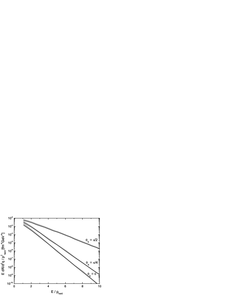
Figure 1: Photon rate for $\xi=10$ and $\alpha_{s}=0.32$ as a function of energy for three different photon angles, $\theta_{q}=\{0,\pi/4,\pi/2\}$, corresponding to rapidities $y=\{\infty,0.88,0\}$, respectively.

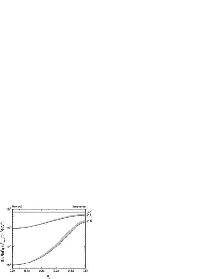
Figure 2: Photon rate for $\xi=\{0,1,10\}$ as a function of the photon angle, $\theta_{q}$, for $E/p_{\rm hard}=5$ and $\alpha_{s}=0.32$.

In Fig. 1 we plot the dependence of the total anisotropic photon production rate as a function of photon energy, $E$, for three different photon propagation angles assuming $\xi=10$ and $\alpha_{s}=0.32$. This Figure shows that there is a clear dependence of the spectrum on photon angle with the difference increasing as the energy of the photon increases. The shaded bands indicate our estimated theoretical uncertainty which is determined by varying the hard-soft separation scale $p^{*}$ by a factor of two around its central value which is parametrically $p^{*}\sim\sqrt{g}\,p_{\rm hard}$. We have scaled everywhere by the arbitrary hard-momentum scale $p_{\rm hard}$ which appears in the quark and gluon distribution functions. This scale will be time dependent with its value set to the nuclear saturation scale, $Q_{s}$, at early times and to the plasma temperature at late times. For RHIC $Q_{s}\sim 1.4\!-\!2\;{\rm GeV}$ and expected initial plasma temperatures are $T_{o}\sim 300\!-\!400\;{\rm MeV}$.

To compare the angular dependence at different $\xi$ in Fig. 2 we show the dependence of the photon production rate on angle at a fixed photon energy $E/p_{\rm hard}=5$ and $\alpha_{s}=0.32$. As can be seen from Fig. 2 the difference between the forward and transverse production rates increases as $\xi$ increases. To summarize the effect we define the photon anisotropy parameter, ${\cal R}_{\gamma}\equiv\left(dR/d^{3}q|_{\theta_{q}=0}\right)/\left(dR/d^{3}q|_{\theta_{q}=\pi/2}\right)$. This ratio is one at all energies if the plasma is isotropic. For anisotropic plasmas it increases as the anisotropy of the system and/or the energy of the photon increases. Due to the limited experimental rapidity acceptance one could define this ratio at a lower angle, e.g. $\pi/4$. However, the ability to resolve anisotropies increases as the sensitivity to forward angles increases so it is best to compare the most forward photons possible with transverse photon emission.

${\cal R}_{\gamma}$	$\;\xi=0\;$	$\;\xi=1\;$	$\;\xi=10\;$
$\;E/p_{\rm hard}=5\;$	1	4.7	$2\cdot 10^{2}$
$\;E/p_{\rm hard}=10\;$	1	34	$3\cdot 10^{4}$

Table 1: Photon anisotropy parameter ${\cal R}_{\gamma}$ for different photon energies and $\xi$, assuming $\alpha_{s}=0.32$.

IV Conclusions and Discussion

The results presented in the previous section demonstrate that the differential high-energy medium photon production rate is sensitive to quark-gluon plasma momentum-space anisotropies with the sensitivity increasing with photon energy. Turning this into the final expected experimental yields as a function of photon energy and angle will require folding this rate together with a phenomenological model of the time dependence of $\xi$ and $p_{\rm hard}$. Current models of plasma evolution do not take into account the evolution of the momentum-space anisotropy of the parton distribution functions. They therefore implicitly assume an isotropic thermal plasma at all times so it will be necessary to extend these models to include the time dependence of $\xi$ and $p_{\rm hard}$. However, since high-energy medium photon production is dominated by early times these photons will be mostly sensitive to the first 1-2 fm/c of plasma evolution where simple models will hopefully be efficacious.

One theoretical shortcoming of our calculation is that it does not include the bremsstrahlung contribution which in an equilibrium plasma also contributes at leading order in the coupling constant due to enhancements from collinear photon radiation Aurenche et al. (1998, 2000); Arnold et al. (2001a, b). This contribution has been omitted because it is currently not known how to resolve the problem that the presence of unstable modes causes unregulated singularities to appear in matrix elements which involve soft gluon exchange. Recent work Romatschke (2006) has suggested that these singularities could be shielded by next-to-leading order corrections to the gluonic polarization tensor, however, the detailed evaluation of these NLO corrections has not been performed to date. Absent an explicit calculation our naive expectation would be that these NLO corrections would yield similar angular dependence since they are also peaked at nearly collinear angles.

References

- Baier et al. (2001) R. Baier, A. H. Mueller, D. Schiff, and D. T. Son, Phys. Lett. B502, 51 (2001), eprint hep-ph/0009237.
- Mrowczynski and Thoma (2000) S. Mrowczynski and M. H. Thoma, Phys. Rev. D62, 036011 (2000), eprint hep-ph/0001164.
- Randrup and Mrowczynski (2003) J. Randrup and S. Mrowczynski, Phys. Rev. C68, 034909 (2003), eprint nucl-th/0303021.
- Romatschke and Strickland (2003) P. Romatschke and M. Strickland, Phys. Rev. D68, 036004 (2003), eprint hep-ph/0304092.
- Arnold et al. (2003) P. Arnold, J. Lenaghan, and G. D. Moore, JHEP 08, 002 (2003), eprint hep-ph/0307325.
- Romatschke and Strickland (2004) P. Romatschke and M. Strickland, Phys. Rev. D70, 116006 (2004), eprint hep-ph/0406188.
- Mrowczynski et al. (2004) S. Mrowczynski, A. Rebhan, and M. Strickland, Phys. Rev. D70, 025004 (2004), eprint hep-ph/0403256.
- Arnold et al. (2005) P. Arnold, G. D. Moore, and L. G. Yaffe, Phys. Rev. D72, 054003 (2005), eprint hep-ph/0505212.
- Rebhan et al. (2005) A. Rebhan, P. Romatschke, and M. Strickland, JHEP 09, 041 (2005), eprint hep-ph/0505261.
- Romatschke and Venugopalan (2006a) P. Romatschke and R. Venugopalan, Phys. Rev. Lett. 96, 062302 (2006a), eprint hep-ph/0510121.
- Schenke et al. (2006) B. Schenke, M. Strickland, C. Greiner, and M. H. Thoma, Phys. Rev. D73, 125004 (2006), eprint hep-ph/0603029.
- Manuel and Mrowczynski (2006) C. Manuel and S. Mrowczynski, Phys. Rev. D74, 105003 (2006), eprint hep-ph/0606276.
- Romatschke and Venugopalan (2006b) P. Romatschke and R. Venugopalan, Phys. Rev. D74, 045011 (2006b), eprint hep-ph/0605045.
- Romatschke and Rebhan (2006) P. Romatschke and A. Rebhan (2006), eprint hep-ph/0605064.
- Dumitru et al. (2006) A. Dumitru, Y. Nara, and M. Strickland (2006), eprint hep-ph/0604149.
- Shuryak (1978) E. V. Shuryak, Phys. Lett. B78, 150 (1978).
- Kajantie and Miettinen (1981) K. Kajantie and H. I. Miettinen, Zeit. Phys. C9, 341 (1981).
- Kapusta et al. (1991) J. I. Kapusta, P. Lichard, and D. Seibert, Phys. Rev. D44, 2774 (1991).
- Redlich et al. (1992) K. Redlich, R. Baier, H. Nakkagawa, and A. Niegawa, Nucl. Phys. A544, 511 (1992).
- Aurenche et al. (1998) P. Aurenche, F. Gelis, R. Kobes, and H. Zaraket, Phys. Rev. D58, 085003 (1998), eprint hep-ph/9804224.
- Aurenche et al. (2000) P. Aurenche, F. Gelis, and H. Zaraket, Phys. Rev. D61, 116001 (2000), eprint hep-ph/9911367.
- Arnold et al. (2001a) P. Arnold, G. D. Moore, and L. G. Yaffe, JHEP 11, 057 (2001a), eprint hep-ph/0109064.
- Arnold et al. (2001b) P. Arnold, G. D. Moore, and L. G. Yaffe, JHEP 12, 009 (2001b), eprint hep-ph/0111107.
- Braaten and Yuan (1991) E. Braaten and T. C. Yuan, Phys. Rev. Lett. 66, 2183 (1991).
- Keldysh (1964) L. Keldysh, Zh. Eks. Teor. Fiz. 47, 1515 (1964).
- Keldysh (1965) L. Keldysh, Sov. Phys. JETP 20, 1018 (1965).
- Chou et al. (1985) K.-c. Chou, Z.-b. Su, B.-l. Hao, and L. Yu, Phys. Rept. 118, 1 (1985).
- Mrowczynski and Heinz (1994) S. Mrowczynski and U. W. Heinz, Ann. Phys. 229, 1 (1994).
- Calzetta and Hu (1988) E. Calzetta and B. L. Hu, Phys. Rev. D37, 2878 (1988).
- Baier et al. (1997) R. Baier, M. Dirks, K. Redlich, and D. Schiff, Phys. Rev. D56, 2548 (1997), eprint hep-ph/9704262.
- Schenke and Strickland (2006) B. Schenke and M. Strickland, Phys. Rev. D74, 065004 (2006), eprint hep-ph/0606160.
- Romatschke (2006) P. Romatschke (2006), eprint hep-ph/0607327.