Abstract

New results for the complete one-loop contributions to the masses and mixing effects in the Higgs sector are obtained for the MSSM with complex parameters using the Feynman-diagrammatic approach. The full dependence on all relevant complex phases is taken into account, and all the imaginary parts appearing in the calculation are treated in a consistent way. The renormalization is discussed in detail, and a hybrid on-shell/$\overline{\mathrm{DR}}$ scheme is adopted. We also derive the wave function normalization factors needed in processes with external Higgs bosons and discuss effective couplings incorporating leading higher-order effects. The complete one-loop corrections, supplemented by the available two-loop corrections in the Feynman-diagrammatic approach for the MSSM with real parameters and a resummation of the leading (s)bottom corrections for complex parameters, are implemented into the public Fortran code FeynHiggs 2.5. In our numerical analysis the full results for the Higgs-boson masses and couplings are compared with various approximations, and ${\cal CP}$-violating effects in the mixing of the heavy Higgs bosons are analyzed in detail. We find sizable deviations in comparison with the approximations often made in the literature.

1 Introduction

A striking prediction of models of supersymmetry (SUSY) [1] is a Higgs sector with at least one relatively light Higgs boson. In the Minimal Supersymmetric extension of the Standard Model (MSSM) two Higgs doublets are required, resulting in five physical Higgs bosons: the light and heavy ${\cal CP}$-even $h$ and $H$, the ${\cal CP}$-odd $A$, and the charged Higgs bosons $H^{\pm}$. The Higgs sector of the MSSM can be expressed at lowest order in terms of $M_{Z}$ (or $M_{W}$), $M_{A}$ (or $M_{H^{\pm}}$) and $\tan\beta\equiv v_{2}/v_{1}$, the ratio of the two vacuum expectation values. All other masses and mixing angles can therefore be predicted. Higher-order contributions give large corrections to the tree-level relations.

The limits obtained from the Higgs search at LEP (the final LEP results can be found in Refs. [2, 3]), place important restrictions on the parameter space of the MSSM. The results obtained so far at Run II of the Tevatron [4, 5, 6] yield interesting constraints in particular in the region of small $M_{A}$ and large $\tan\beta$ (the dependence on the other MSSM parameters has recently been analyzed in Ref. [7]). The Large Hadron Collider (LHC) has good prospects for the discovery of at least one Higgs boson over all the MSSM parameter space [8, 9, 10] (see e.g. Refs. [11, 12] for recent reviews). At the International Linear Collider (ILC) eventually high-precision physics in the Higgs sector may become possible [13, 14, 15]. The interplay of the LHC and the ILC in the MSSM Higgs sector is discussed in Refs. [16, 17].

For the MSSM with real parameters (rMSSM) the status of higher-order corrections to the masses and mixing angles in the Higgs sector is quite advanced. The complete one-loop result within the rMSSM is known [18, 19, 20, 21]. The by far dominant one-loop contribution is the ${\cal O}(\alpha_{t})$ term due to top and stop loops ($\alpha_{t}\equiv h_{t}^{2}/(4\pi)$, $h_{t}$ being the top-quark Yukawa coupling). The computation of the two-loop corrections has meanwhile reached a stage where all the presumably dominant contributions are available [22, 23, 24, 25, 26, 27, 28, 29, 30, 31, 32, 33, 34, 35, 36]. In particular, the ${\cal O}(\alpha_{t}\alpha_{s})$, ${\cal O}(\alpha_{t}^{2})$, ${\cal O}(\alpha_{b}\alpha_{s})$, ${\cal O}(\alpha_{t}\alpha_{b})$ and ${\cal O}(\alpha_{b}^{2})$ contributions to the self-energies are known for vanishing external momenta. For the (s)bottom corrections, which are mainly relevant for large values of $\tan\beta$, an all-order resummation of the $\tan\beta$-enhanced term of ${\cal O}(\alpha_{b}(\alpha_{s}\tan\beta)^{n})$ is performed [37, 38, 39, 40]. The remaining theoretical uncertainty on the lightest ${\cal CP}$-even Higgs boson mass has been estimated to be below $\sim 3\,\,\mathrm{GeV}$ [41, 42, 43]. The above calculations have been implemented into public codes. The program FeynHiggs [23, 44, 45, 46] is based on the results obtained in the Feynman-diagrammatic (FD) approach [22, 23, 41, 34]. It includes all the above corrections. The code CPsuperH [47] is based on the renormalization group (RG) improved effective potential approach [36, 35, 26]. Most recently a full two-loop effective potential calculation (including even the momentum dependence for the leading pieces) has been published [49]. However, no computer code is publicly available. Besides the masses in the Higgs sector, also for the couplings of the rMSSM Higgs bosons to SM bosons and fermions detailed higher-order corrections are available [50, 37, 38, 39, 51].

In the case of the MSSM with complex parameters (cMSSM) the higher order corrections have yet been restricted, after the first more general investigations [52], to evaluations in the effective potential (EP) approach [53, 54] (at one-loop, neglecting the momentum-dependent effects) and to the RG improved one-loop EP method [55, 56]. The latter ones have been restricted to the corrections arising from the (s)fermion sector and some leading logarithmic corrections from the gaugino sector. Within the FD approach the one-loop leading $m_{t}^{4}$ corrections have been evaluated in Ref. [57]. Effects of imaginary parts of the one-loop contributions to Higgs boson masses and couplings have been considered in Refs. [58, 59, 60]. Further discussions on the effect of complex phases on Higgs boson masses and decays can be found in Refs. [61, 62, 63, 64]. A detailed comparison between the two available computer codes for the cMSSM Higgs-boson sector, FeynHiggs and CPsuperH, will be performed in a forthcoming publication.

In the present paper we present the complete one-loop evaluation of the Higgs-boson masses and mixings in the cMSSM (see Ref. [65] for preliminary results). The full phase dependence, the full momentum dependence and the effects of imaginary parts of the Higgs-boson self-energies are taken consistently into account. Our results are based on the FD approach using a hybrid renormalization scheme where the masses are renormalized on-shell, while the $\overline{\mathrm{DR}}$ scheme is applied for $\tan\beta$ and the field renormalizations. The higher-order self-energy corrections are utilized to obtain wave function normalization factors for external Higgs bosons and to discuss effective couplings incorporating leading higher-order effects. We provide numerical examples for the lightest cMSSM Higgs boson, the mass difference of the heavier neutral Higgses and for the mixing between the three neutral Higgs bosons. We compare our results with various approximations often made in the literature. All results are incorporated into the public Fortran code FeynHiggs 2.5 [23, 44, 45, 46].

The rest of the paper is organized as follows. In Sect. 2 we review all relevant sectors of the cMSSM. Besides the tree-level structure of the Higgs sector, the renormalization necessary for the one-loop calculations is explained in detail. In Sect. 3 the evaluation of the one-loop self-energies is presented. The determination of the Higgs-boson masses from the propagators and of wave function normalization factors and effective couplings is described. Our numerical analysis is given in Sect. 4. Information about the Fortran code FeynHiggs 2.5 is provided in Sect. 5, more details about installation and use are given in the Appendix. We conclude with Sect. 6.

2 Calculational basis

2.1 The scalar quark sector in the cMSSM

The mass matrix of two squarks of the same flavor, $\tilde{q}_{L}$ and $\tilde{q}_{R}$, is given by

$$M_{\tilde{q}}=\begin{pmatrix}M_{L}^{2}+m_{q}^{2}+M_{Z}^{2}\cos 2\beta(I_{3}^{q}-Q_{q}s_{\mathrm{w}}^{2})&m_{q}\;X_{q}^{*}\\ m_{q}\;X_{q}&M_{\tilde{q}_{R}}^{2}+m_{q}^{2}+M_{Z}^{2}\cos 2\beta Q_{q}s_{\mathrm{w}}^{2}\end{pmatrix},$$ (1)

with

$$X_{q} = A_{q}-\mu^{*}\{\cot\beta,\tan\beta\},$$ (2)

where $\{\cot\beta,\tan\beta\}$ applies for up- and down-type squarks, respectively, the star denotes a complex conjugation, and $\tan\beta\equiv v_{2}/v_{1}$. In Eq. (2) $M_{L}^{2}$, $M_{\tilde{q}_{R}}^{2}$ are real soft SUSY-breaking parameters, while the soft SUSY-breaking trilinear coupling $A_{q}$ and the higgsino mass parameter $\mu$ can be complex. As a consequence, in the scalar quark sector of the cMSSM $N_{q}+1$ phases are present, one for each $A_{q}$ and one for $\mu$, i.e. $N_{q}+1$ new parameters appear. As an abbreviation we will use

$$\varphi_{X_{q}}\equiv{\rm arg}\left(X_{q}\right),\;\varphi_{A_{q}}\equiv\arg\left(A_{q}\right)~{}.$$ (3)

One can trade $\varphi_{A_{q}}$ for $\varphi_{X_{q}}$ as independent parameter.
The squark mass eigenstates are obtained by the unitary transformation

$$\left(\begin{array}[]{c}\tilde{q}_{1}\\ \tilde{q}_{2}\end{array}\right)={\mathbf{U}}_{\tilde{q}}\left(\begin{array}[]{c}\tilde{q}_{L}\\ \tilde{q}_{R}\end{array}\right)$$ (4)

with

$${\mathbf{U}}_{\tilde{q}}=\left(\begin{array}[]{cc}c_{\tilde{q}}&s_{\tilde{q}}\\ -s_{\tilde{q}}^{*}&c_{\tilde{q}}\end{array}\right),\quad{\mathbf{U}}_{\tilde{q}}{\mathbf{U}}_{\tilde{q}}^{\dagger}={\rm 1\mskip-4.25mul}~{},$$ (5)

The elements of the mixing matrix ${\mathbf{U}}$ can be calculated as

$$c_{\tilde{q}} =\frac{\sqrt{M_{L}^{2}+m_{q}^{2}+M_{Z}^{2}\cos 2\beta(I_{3}^{q}-Q_{q}s_{\mathrm{w}}^{2})-m_{\tilde{q}_{2}}^{2}}}{\sqrt{m_{\tilde{q}_{1}}^{2}-m_{\tilde{q}_{2}}^{2}}},$$ (6)

$$s_{\tilde{q}} =\frac{m_{q}X_{q}^{*}}{\sqrt{M_{L}^{2}+M_{Z}^{2}\cos 2\beta(I_{3}^{q}-Q_{q}s_{\mathrm{w}}^{2})+m_{q}^{2}-m_{\tilde{q}_{2}}^{2}}\sqrt{m_{\tilde{q}_{1}}^{2}-m_{\tilde{q}_{2}}^{2}}}.$$ (7)

Here $c_{\tilde{q}}\equiv\cos\theta\kern-1.49994pt_{\tilde{q}}$ is real, whereas $s_{\tilde{q}}\equiv e^{-i\varphi_{X_{q}}}\,\sin\theta\kern-1.49994pt_{\tilde{q}}$ can be complex with the phase

$$\varphi_{s_{\tilde{q}}}=-\varphi_{X_{q}}={\rm arg}\left(X_{q}^{*}\right)~{}.$$ (8)

The mass eigenvalues are given by

$$m_{\tilde{q}_{1,2}}^{2}=m_{q}^{2}+\frac{1}{2} \Bigl{[}M_{L}^{2}+M_{\tilde{q}_{R}}^{2}+I_{3}^{q}M_{Z}^{2}\cos 2\beta$$ (9)

$$\mp\sqrt{[M_{L}^{2}-M_{\tilde{q}_{R}}^{2}+M_{Z}^{2}\cos 2\beta(I_{3}^{q}-2Q_{q}s_{\mathrm{w}}^{2})]^{2}+4m_{q}^{2}|X_{q}|^{2}}~{}\Bigr{]},$$ (10)

and are independent of the phase of $X_{q}$.

2.2 The chargino / neutralino sector of the cMSSM

The mass eigenstates of the charginos can be determined from the matrix

$${\mathbf{X}}=\begin{pmatrix}M_{2}&\sqrt{2}\sin\beta\,M_{W}\\ \sqrt{2}\cos\beta\,M_{W}&\mu\end{pmatrix}.$$ (11)

In addition to the higgsino mass parameter $\mu$ it contains the soft breaking term $M_{2}$, which can also be complex in the cMSSM. The rotation to the chargino mass eigenstates is done by transforming the original wino and higgsino fields with the help of two unitary 2$\times$2 matrices ${\mathbf{U}}$ and ${\mathbf{V}}$,

$$\begin{pmatrix}\tilde{\chi}_{1}^{+}\\ \tilde{\chi}_{2}^{+}\end{pmatrix}={\mathbf{V}}\begin{pmatrix}\tilde{W}^{+}\\ \tilde{H}_{2}^{+}\end{pmatrix},\quad\begin{pmatrix}\tilde{\chi}_{1}^{-}\\ \tilde{\chi}_{2}^{-}\end{pmatrix}={\mathbf{U}}\begin{pmatrix}\tilde{W}^{-}\\ \tilde{H}_{1}^{-}\end{pmatrix}.$$ (12)

These rotations lead to the diagonal mass matrix

$$\begin{pmatrix}m_{\tilde{\chi}^{\pm}_{1}}&0\\ 0&m_{\tilde{\chi}^{\pm}_{2}}\end{pmatrix}={\mathbf{U}}^{*}\,{\mathbf{X}}\,{\mathbf{V}}^{\dagger}.$$ (13)

From this relation, it becomes clear that the chargino masses $m_{\tilde{\chi}^{\pm}_{1}}$ and $m_{\tilde{\chi}^{\pm}_{2}}$ can be determined as the (real and positive) singular values of ${\mathbf{X}}$. The singular value decomposition of ${\mathbf{X}}$ also yields results for ${\mathbf{U}}$ and ${\mathbf{V}}$.

A similar procedure is used for the determination of the neutralino masses and mixing matrix, which can both be calculated from the mass matrix

$${\mathbf{Y}}=\begin{pmatrix}M_{1}&0&-M_{Z}\,s_{\mathrm{w}}\cos\beta\,&M_{Z}\,s_{\mathrm{w}}\sin\beta\,\\ 0&M_{2}&\quad M_{Z}\,c_{\mathrm{w}}\cos\beta\,&M_{Z}\,c_{\mathrm{w}}\sin\beta\,\\ -M_{Z}\,s_{\mathrm{w}}\cos\beta\,&M_{Z}\,c_{\mathrm{w}}\cos\beta\,&0&-\mu\\ \quad M_{Z}\,s_{\mathrm{w}}\sin\beta\,&M_{Z}\,c_{\mathrm{w}}\sin\beta\,&-\mu&0\end{pmatrix}.$$ (14)

This symmetric matrix contains the additional complex soft-breaking parameter $M_{1}$. The diagonalization of the matrix is achieved by a transformation starting from the original bino/wino/higgsino basis,

$$\begin{pmatrix}\tilde{\chi}^{0}_{1}\\[5.0pt] \tilde{\chi}^{0}_{2}\\[5.0pt] \tilde{\chi}^{0}_{3}\\[5.0pt] \tilde{\chi}^{0}_{4}\end{pmatrix}={\mathbf{N}}\begin{pmatrix}\tilde{B}^{0}\\[5.0pt] \tilde{W}^{0}\\[5.0pt] \tilde{H}_{1}^{0}\\[5.0pt] \tilde{H}_{2}^{0}\end{pmatrix},\quad\begin{pmatrix}m_{\tilde{\chi}^{0}_{1}}&0&0&0\\[5.0pt] 0&m_{\tilde{\chi}^{0}_{2}}&0&0\\[5.0pt] 0&0&m_{\tilde{\chi}^{0}_{3}}&0\\[5.0pt] 0&0&0&m_{\tilde{\chi}^{0}_{4}}\end{pmatrix}={\mathbf{N}}^{*}\,{\mathbf{Y}}\,{\mathbf{N}}^{\dagger}.$$ (15)

The unitary 4$\times$4 matrix ${\mathbf{N}}$ and the physical neutralino masses again result from a numerical singular value decomposition of ${\mathbf{Y}}$. The symmetry of ${\mathbf{Y}}$ permits the non-trivial condition of using only one matrix ${\mathbf{N}}$ for its diagonalization, in contrast to the chargino case shown above.

2.3 The cMSSM Higgs potential

The Higgs potential $V_{H}$ contains the real soft breaking terms $\tilde{m}_{1}^{2}$ and $\tilde{m}_{2}^{2}$ (with $m_{1}^{2}\equiv\tilde{m}_{1}^{2}+|\mu|^{2}$, $m_{2}^{2}\equiv\tilde{m}_{2}^{2}+|\mu|^{2}$), the potentially complex soft breaking parameter $m_{12}^{2}$, and the U$(1)$ and SU$(2)$ coupling constants $g_{1}$ and $g_{2}$:

$$V_{H} =m_{1}^{2}H_{1i}^{*}H_{1i}+m_{2}^{2}H_{2i}^{*}H_{2i}-\epsilon^{ij}(m_{12}^{2}H_{1i}H_{2j}+{m_{12}^{2}}^{*}H_{1i}^{*}H_{2j}^{*})$$

$$\quad+\tfrac{1}{8}(g_{1}^{2}+g_{2}^{2})(H_{1i}^{*}H_{1i}-H_{2i}^{*}H_{2i})^{2}+\tfrac{1}{2}g_{2}^{2}|H_{1i}^{*}H_{2i}|^{2}.$$ (16)

The indices $\{i,j\}=\{1,2\}$ refer to the respective Higgs doublet component (summation over $i$ and $j$ is understood), and $\epsilon^{12}=1$. The Higgs doublets are decomposed in the following way,

$${\cal H}_{1}=\begin{pmatrix}H_{11}\\ H_{12}\end{pmatrix} =\begin{pmatrix}v_{1}+\tfrac{1}{\sqrt{2}}(\phi_{1}-i\chi_{1})\\ -\phi^{-}_{1}\end{pmatrix},$$

$${\cal H}_{2}=\begin{pmatrix}H_{21}\\ H_{22}\end{pmatrix} =e^{i\xi}\begin{pmatrix}\phi^{+}_{2}\\ v_{2}+\tfrac{1}{\sqrt{2}}(\phi_{2}+i\chi_{2})\end{pmatrix}.$$ (17)

Besides the vacuum expectation values $v_{1}$ and $v_{2}$, eq. (2.3) introduces a possible new phase $\xi$ between the two Higgs doublets. Using this decomposition, $V_{H}$ can be rearranged in powers of the fields,

$$V_{H} =\cdots-T_{\phi_{1}}\phi_{1}-T_{\phi_{2}}\phi_{2}-T_{\chi_{1}}\chi_{1}-T_{\chi_{2}}\chi_{2}+$$

$$+\tfrac{1}{2}\begin{pmatrix}\phi_{1},\phi_{2},\chi_{1},\chi_{2}\end{pmatrix}{\mathbf{M}}_{\phi\phi\chi\chi}\begin{pmatrix}\phi_{1}\\ \phi_{2}\\ \chi_{1}\\ \chi_{2}\end{pmatrix}+\begin{pmatrix}\phi^{-}_{1},\phi^{-}_{2}\end{pmatrix}{\mathbf{M}}_{\phi^{\pm}\phi^{\pm}}\begin{pmatrix}\phi^{+}_{1}\\ \phi^{+}_{2}\end{pmatrix}+\cdots,$$ (18)

where the coefficients of the linear terms are called tadpoles and those of the bilinear terms are the mass matrices ${\mathbf{M}}_{\phi\phi\chi\chi}$ and ${\mathbf{M}}_{\phi^{\pm}\phi^{\pm}}$. The tadpole coefficients read

$$T_{\phi_{1}} =-\sqrt{2}(m_{1}^{2}v_{1}-\cos\xi^{\prime}|m_{12}^{2}|v_{2}+\tfrac{1}{4}(g_{1}^{2}+g_{2}^{2})(v_{1}^{2}-v_{2}^{2})v_{1}),$$ (19a)

$$T_{\phi_{2}} =-\sqrt{2}(m_{2}^{2}v_{2}-\cos\xi^{\prime}|m_{12}^{2}|v_{1}-\tfrac{1}{4}(g_{1}^{2}+g_{2}^{2})(v_{1}^{2}-v_{2}^{2})v_{2}),$$ (19b)

$$T_{\chi_{1}} =\sqrt{2}\sin\xi^{\prime}|m_{12}^{2}|v_{2}=-T_{\chi_{2}}\frac{v_{2}}{v_{1}},$$ (19c)

with $\xi^{\prime}\equiv\xi+\arg(m_{12}^{2})$.

With the help of a Peccei-Quinn transformation [66] $\mu$ and $m_{12}^{2}$ can be redefined [67] such that the complex phase of $m_{12}^{2}$ vanishes. In the following we will therefore treat $m_{12}^{2}$ as a real parameter, which yields

$$|m_{12}^{2}|=m_{12}^{2},\quad\xi^{\prime}=\xi.$$ (20)

The real, symmetric 4$\times$4-matrix ${\mathbf{M}}_{\phi\phi\chi\chi}$ and the hermitian 2$\times$2-matrix ${\mathbf{M}}_{\phi^{\pm}\phi^{\pm}}$ contain the following elements,

$${\mathbf{M}}_{\phi\phi\chi\chi} =\begin{pmatrix}{\mathbf{M}}_{\phi}&{\mathbf{M}}_{\phi\chi}\\[5.0pt] {\mathbf{M}}_{\phi\chi}^{\dagger}&{\mathbf{M}}_{\chi}\end{pmatrix},$$ (21a)

$${\mathbf{M}}_{\phi} =\begin{pmatrix}m_{1}^{2}+\tfrac{1}{4}(g_{1}^{2}+g_{2}^{2})(3v_{1}^{2}-v_{2}^{2})&-\cos\xi\,m_{12}^{2}-\tfrac{1}{2}(g_{1}^{2}+g_{2}^{2})v_{1}v_{2}\\[5.0pt] -\cos\xi\,m_{12}^{2}-\tfrac{1}{2}(g_{1}^{2}+g_{2}^{2})v_{1}v_{2}&m_{2}^{2}+\tfrac{1}{4}(g_{1}^{2}+g_{2}^{2})(3v_{2}^{2}-v_{1}^{2})\end{pmatrix},$$ (21b)

$${\mathbf{M}}_{\phi\chi} =\begin{pmatrix}0&\sin\xi\,m_{12}^{2}\\[5.0pt] -\sin\xi\,m_{12}^{2}&0\end{pmatrix},$$ (21c)

$${\mathbf{M}}_{\chi} =\begin{pmatrix}m_{1}^{2}+\tfrac{1}{4}(g_{1}^{2}+g_{2}^{2})(v_{1}^{2}-v_{2}^{2})&-\cos\xi\,m_{12}^{2}\\[5.0pt] -\cos\xi\,m_{12}^{2}&m_{2}^{2}+\tfrac{1}{4}(g_{1}^{2}+g_{2}^{2})(v_{2}^{2}-v_{1}^{2})\end{pmatrix},$$ (21d)

$${\mathbf{M}}_{\phi^{\pm}\phi^{\pm}} =\begin{pmatrix}m_{1}^{2}+\tfrac{1}{4}g_{1}^{2}(v_{1}^{2}-v_{2}^{2})+\tfrac{1}{4}g_{2}^{2}(v_{1}^{2}+v_{2}^{2})&-e^{i\xi}m_{12}^{2}-\tfrac{1}{2}g_{2}^{2}v_{1}v_{2}\\[5.0pt] -e^{-i\xi}m_{12}^{2}-\tfrac{1}{2}g_{2}^{2}v_{1}v_{2}&m_{2}^{2}+\tfrac{1}{4}g_{1}^{2}(v_{2}^{2}-v_{1}^{2})+\tfrac{1}{4}g_{2}^{2}(v_{1}^{2}+v_{2}^{2})\end{pmatrix}.$$ (21e)

The non-vanishing elements of ${\mathbf{M}}_{\phi\chi}$ lead to ${\cal CP}$-violating mixing terms in the Higgs potential between the ${\cal CP}$-even fields $\phi_{1}$ and $\phi_{2}$ and the ${\cal CP}$-odd fields $\chi_{1}$ and $\chi_{2}$ if $\xi\neq 0$. The mass eigenstates in lowest order follow from unitary transformations on the original fields,

$$\begin{pmatrix}h\\ H\\ A\\ G\end{pmatrix}={\mathbf{U}}_{\mathrm{n}(0)}\cdot\begin{pmatrix}\phi_{1}\\ \phi_{2}\\ \chi_{1}\\ \chi_{2}\end{pmatrix},\quad\begin{pmatrix}H^{\pm}\\ G^{\pm}\end{pmatrix}={\mathbf{U}}_{\mathrm{c}(0)}\cdot\begin{pmatrix}\phi_{1}^{\pm}\\ \phi_{2}^{\pm}\end{pmatrix}.$$ (22)

The matrices ${\mathbf{U}}_{\mathrm{n}(0)}$ and ${\mathbf{U}}_{\mathrm{c}(0)}$ transform the neutral and charged Higgs fields, respectively, such that the resulting mass matrices

$${\mathbf{M}}_{hHAG}^{\rm diag}={\mathbf{U}}_{\mathrm{n}(0)}{\mathbf{M}}_{\phi\phi\chi\chi}{\mathbf{U}}_{\mathrm{n}(0)}^{\dagger}\quad{\rm and}\quad{\mathbf{M}}_{H^{\pm}G^{\pm}}^{\rm diag}={\mathbf{U}}_{\mathrm{c}(0)}{\mathbf{M}}_{\phi^{\pm}\phi^{\pm}}{\mathbf{U}}_{\mathrm{c}(0)}^{\dagger}$$ (23)

are diagonal in the basis of the transformed fields. The new fields correspond to the three neutral Higgs bosons $h$, $H$ and $A$, the charged pair $H^{\pm}$ and the Goldstone bosons $G$ and $G^{\pm}$.

The lowest-order mixing matrices can be determined from the eigenvectors of ${\mathbf{M}}_{\phi\phi\chi\chi}$ and ${\mathbf{M}}_{\phi^{\pm}\phi^{\pm}}$, calculated under the additional condition that the tadpole coefficients (19) must vanish in order that $v_{1}$ and $v_{2}$ are indeed stationary points of the Higgs potential. This automatically requires $\xi=0$, which in turn leads to a vanishing matrix ${\mathbf{M}}_{\phi\chi}$ and a real, symmetric matrix ${\mathbf{M}}_{\phi^{\pm}\phi^{\pm}}$. Therefore, no ${\cal CP}$-violation occurs in the Higgs potential at the lowest order, and the corresponding mixing matrices can be parametrized by real mixing angles as

$${\mathbf{U}}_{\mathrm{n}(0)}=\begin{pmatrix}-\sin\alpha\,&\cos\alpha\,&0&0\\ \quad\cos\alpha\,&\sin\alpha\,&0&0\\ 0&0&-\sin\beta_{\mathrm{n}}&\cos\beta_{\mathrm{n}}\\ 0&0&\quad\cos\beta_{\mathrm{n}}&\sin\beta_{\mathrm{n}}\end{pmatrix},\quad{\mathbf{U}}_{\mathrm{c}(0)}=\begin{pmatrix}-\sin\beta_{\mathrm{c}}&\cos\beta_{\mathrm{c}}\\ \quad\cos\beta_{\mathrm{c}}&\sin\beta_{\mathrm{c}}\end{pmatrix}.$$ (24)

The mixing angles $\alpha$, $\beta_{\mathrm{n}}$ and $\beta_{\mathrm{c}}$ can be determined from the requirement that this transformation results in diagonal mass matrices for the physical fields. It is necessary, however, to determine the elements of the mass matrices without inserting the explicit form of the mixing angles and keeping the dependence on the complex phase $\xi$, since these expressions will be needed for the renormalization of the Higgs potential and the calculation of the tadpole and mass counterterms at one-loop order.

2.4 Higgs mass terms and tadpoles

In order to specify our notation and the conventions used in this paper we write out the Higgs mass terms and tadpole terms in detail. The terms in $V_{H}$, expressed in the mass eigenstate basis, which are linear or quadratic in the fields are denoted as follows,

$$V_{H} =\mathrm{const.}-T_{h}\cdot h-T_{H}\cdot H-T_{A}\cdot A-T_{G}\cdot G$$

$$\quad+\tfrac{1}{2}\begin{pmatrix}h,H,A,G\end{pmatrix}\cdot\begin{pmatrix}m_{h}^{2}&m_{hH}^{2}&m_{hA}^{2}&m_{hG}^{2}\\ m_{hH}^{2}&m_{H}^{2}&m_{HA}^{2}&m_{HG}^{2}\\ m_{hA}^{2}&m_{HA}^{2}&m_{A}^{2}&m_{AG}^{2}\\ m_{hG}^{2}&m_{HG}^{2}&m_{AG}^{2}&m_{G}^{2}\end{pmatrix}\cdot\begin{pmatrix}h\\ H\\ A\\ G\end{pmatrix}+$$ (25)

$$\quad+\begin{pmatrix}H^{-},G^{-}\end{pmatrix}\cdot\begin{pmatrix}m_{H^{\pm}}^{2}&m_{H^{-}G^{+}}^{2}\\ m_{G^{-}H^{+}}^{2}&m_{G^{\pm}}^{2}\end{pmatrix}\cdot\begin{pmatrix}H^{+}\\ G^{+}\end{pmatrix}+\cdots.$$

Our notation for the Higgs masses in this paper is such that lowest-order mass parameters are written in lower case, e.g. $m_{h}^{2}$, while loop-corrected masses are written in upper case, e.g. $M_{h}^{2}$.

For the gauge-fixing, affecting terms involving Goldstone fields in Eq. (2.4), we have chosen the ’t Hooft–Feynman gauge. In the renormalization we follow the usual approach where the gauge-fixing term receives no net contribution from the renormalization transformations. Accordingly, the counterterms derived below arise only from the Higgs potential and the kinetic terms of the Higgs fields but not from the gauge-fixing term.

In order to perform the renormalization procedure in a transparent way, we express the parameters in $V_{H}$ in terms of physical parameters. In total, $V_{H}$ contains eight independent real parameters: $v_{1}$, $v_{2}$, $g_{1}^{2}$, $g_{2}^{2}$, $m_{1}^{2}$, $m_{2}^{2}$, $m_{12}^{2}$ and $\xi$, which can be replaced by the parameters $M_{Z}$, $M_{W}$, $e$, $m_{H^{\pm}}$ (or $m_{A}$), $\tan\beta$, $T_{h}$, $T_{H}$ and $T_{A}$. Thereby, the coupling constants $g_{1}$ and $g_{2}$ are replaced by the electromagnetic coupling constant $e$ and the weak mixing angle $\theta_{\mathrm{w}}$ in terms of $c_{\mathrm{w}}\equiv\cos\theta_{\mathrm{w}}=M_{W}/M_{Z},s_{\mathrm{w}}=\sqrt{1-c_{\mathrm{w}}^{2}}$,

$$e=g_{1}\,c_{\mathrm{w}}=g_{2}\,s_{\mathrm{w}},$$ (26)

while the $Z$ boson mass $M_{Z}$ and $\tan\beta$ substitute for $v_{1}$ and $v_{2}$:

$$M_{Z}^{2}=\tfrac{1}{2}(g_{1}^{2}+g_{2}^{2})(v_{1}^{2}+v_{2}^{2}),\;\tan\beta=\frac{v_{2}}{v_{1}}.$$ (27)

The $W$ boson mass is then given by

$$M_{W}^{2}=\frac{1}{2}g_{2}^{2}(v_{1}^{2}+v_{2}^{2}).$$ (28)

The tadpole coefficients in the mass-eigenstate basis follow from the original ones (19) by transforming the fields according to Eq. (22),

$$T_{H} =\sqrt{2}(-m_{1}^{2}v_{1}\cos\alpha\,-m_{2}^{2}v_{2}\sin\alpha\,+\cos\xi\,m_{12}^{2}(v_{1}\sin\alpha\,+v_{2}\cos\alpha\,)$$ (29a)

$$\quad-\tfrac{1}{4}(g_{1}^{2}+g_{2}^{2})(v_{1}^{2}-v_{2}^{2})(v_{1}\cos\alpha\,-v_{2}\sin\alpha\,)),$$

$$T_{h} =\sqrt{2}(+m_{1}^{2}v_{1}\sin\alpha\,-m_{2}^{2}v_{2}\cos\alpha\,+\cos\xi\,m_{12}^{2}(v_{1}\cos\alpha\,-v_{2}\sin\alpha\,)$$ (29b)

$$\quad+\tfrac{1}{4}(g_{1}^{2}+g_{2}^{2})(v_{1}^{2}-v_{2}^{2})(v_{1}\sin\alpha\,+v_{2}\cos\alpha\,)),$$

$$T_{A} =-\sqrt{2}\sin\xi\,m_{12}^{2}(v_{1}\cos\beta_{\mathrm{n}}+v_{2}\sin\beta_{\mathrm{n}}),$$ (29c)

$$T_{G} =-\tan(\beta-\beta_{\mathrm{n}})T_{A}.$$ (29d)

Using Eqs. (26) – (29) the original parameters can be expressed in terms of $e$, $\tan\beta$, $M_{Z}$, $M_{W}$, $T_{h}$, $T_{H}$, $T_{A}$ and either the mass of the neutral $A$ boson, $m_{A}$, or the mass of the charged Higgs boson, $m_{H^{\pm}}$ (it should be noted that Eqs. (29a)–(29d) yield only three independent relations because of the linear dependence of $T_{G}$ on $T_{A}$). The masses $m_{A}$ and $m_{H^{\pm}}$ are related to the original parameters by

$$m_{A}^{2} =m_{1}^{2}\sin^{2}\beta_{\mathrm{n}}+m_{2}^{2}\cos^{2}\beta_{\mathrm{n}}+\sin 2\beta_{\mathrm{n}}\cos\xi\,m_{12}^{2}$$

$$\quad-\cos 2\beta_{\mathrm{n}}\tfrac{1}{4}(g_{1}^{2}+g_{2}^{2})(v_{1}^{2}-v_{2}^{2}),$$ (30a)

$$m_{H^{\pm}}^{2} =m_{1}^{2}\sin^{2}\beta_{\mathrm{c}}+m_{2}^{2}\cos^{2}\beta_{\mathrm{c}}+\sin 2\beta_{\mathrm{c}}\cos\xi\,m_{12}^{2}$$

$$\quad-\cos 2\beta_{\mathrm{c}}\tfrac{1}{4}(g_{1}^{2}+g_{2}^{2})(v_{1}^{2}-v_{2}^{2})+\tfrac{1}{2}g_{2}^{2}(v_{1}\cos\beta_{\mathrm{c}}+v_{2}\sin\beta_{\mathrm{c}})^{2}~{}.$$ (30b)

Choosing $m_{A}$ as the independent parameter yields the following relations,

$$v_{1} =\frac{\sqrt{2}\,\cos\beta\,s_{\mathrm{w}}\,c_{\mathrm{w}}\,M_{Z}}{e}$$ (31)

$$v_{2} =\frac{\sqrt{2}\,\sin\beta\,s_{\mathrm{w}}\,c_{\mathrm{w}}\,M_{Z}}{e}$$ (32)

$$g_{1} =e/c_{\mathrm{w}}$$ (33)

$$g_{2} =e/s_{\mathrm{w}}$$ (34)

$$m_{1}^{2} =-\frac{1}{2}M_{Z}^{2}\cos(2\beta)+m_{A}^{2}\sin^{2}\beta/\left(\cos^{2}(\beta-\beta_{\mathrm{n}})\right)$$

$$\quad\ +\Big{[}\frac{eT_{h}\cos\beta_{\mathrm{n}}}{2c_{\mathrm{w}}s_{\mathrm{w}}M_{Z}}\left(\cos\beta\cos\beta_{\mathrm{n}}\sin\alpha+\sin\beta(\cos\alpha\cos\beta_{\mathrm{n}}+2\sin\alpha\sin\beta_{\mathrm{n}})\right)$$

$$\qquad\ -\frac{eT_{H}\cos\beta_{\mathrm{n}}}{2c_{\mathrm{w}}s_{\mathrm{w}}M_{Z}}\left(\cos(\alpha+\beta)\cos\beta_{\mathrm{n}}+2\cos\alpha\sin\beta\sin\beta_{\mathrm{n}}\right)\Big{]}/\left(\cos^{2}(\beta-\beta_{\mathrm{n}})\right)$$ (35)

$$m_{2}^{2} =\frac{1}{2}M_{Z}^{2}\cos(2\beta)+m_{A}^{2}\cos^{2}\beta/\left(\cos^{2}(\beta-\beta_{\mathrm{n}})\right)$$

$$\quad\ -\Big{[}\frac{eT_{H}\sin\beta_{\mathrm{n}}}{2c_{\mathrm{w}}s_{\mathrm{w}}M_{Z}}\left(\sin\alpha\sin\beta\sin\beta_{\mathrm{n}}+\cos\beta(2\cos\beta_{\mathrm{n}}\sin\alpha-\cos\alpha\sin\beta_{\mathrm{n}})\right)$$

$$\qquad\ +\frac{eT_{h}\sin\beta_{\mathrm{n}}}{2c_{\mathrm{w}}s_{\mathrm{w}}M_{Z}}\left(2\cos\alpha\cos\beta\cos\beta_{\mathrm{n}}+\sin(\alpha+\beta)\sin\beta_{\mathrm{n}}\right)\Big{]}/\left(\cos^{2}(\beta-\beta_{\mathrm{n}})\right)$$ (36)

$$m_{12}^{2} =\sqrt{\left(f_{m}^{2}+f_{s}^{2}\right)}$$ (37)

$$\sin\xi \to f_{s}/\sqrt{f_{m}^{2}+f_{s}^{2}}$$ (38)

$$\cos\xi \to f_{m}/\sqrt{f_{m}^{2}+f_{s}^{2}},$$ (39)

where

$$f_{m} = \Big{[}\frac{1}{2}m_{A}^{2}\sin 2\beta+\frac{eT_{h}}{4c_{\mathrm{w}}s_{\mathrm{w}}M_{Z}}\left(\cos(\beta+\alpha)+\cos(\beta-\alpha)\cos(2\beta_{\mathrm{n}})\right)$$ (40)

$${}+\frac{eT_{H}}{4c_{\mathrm{w}}s_{\mathrm{w}}M_{Z}}\left(\sin(\beta+\alpha)-\sin(\beta-\alpha)\cos(2\beta_{\mathrm{n}})\right)\Big{]}/\left(\cos^{2}(\beta-\beta_{\mathrm{n}})\right),$$

$$f_{s} = -\frac{eT_{A}}{2s_{\mathrm{w}}c_{\mathrm{w}}M_{Z}\cos(\beta-\beta_{\mathrm{n}})}.$$ (41)

We now give the bilinear terms of Eq. (2.4) in this basis, expressed in terms of $m_{A}$ or $m_{H^{\pm}}$, depending on which parameter leads to more compact expressions. For the charged Higgs sector this yields, apart from $m_{H^{\pm}}$ itself,

$$m_{H^{-}G^{+}}^{2} =-m_{H^{\pm}}^{2}\tan(\beta-\beta_{\mathrm{c}})$$ (42a)

$$\quad-\frac{e}{2M_{Z}s_{\mathrm{w}}c_{\mathrm{w}}}T_{H}\sin(\alpha-\beta_{\mathrm{c}})/\cos(\beta-\beta_{\mathrm{c}})$$

$$\quad-\frac{e}{2M_{Z}s_{\mathrm{w}}c_{\mathrm{w}}}T_{h}\cos(\alpha-\beta_{\mathrm{c}})/\cos(\beta-\beta_{\mathrm{c}})$$

$$\quad-\frac{e}{2M_{Z}s_{\mathrm{w}}c_{\mathrm{w}}}iT_{A}/\cos(\beta-\beta_{\mathrm{n}}),$$

$$m_{G^{-}H^{+}}^{2} =(m_{H^{-}G^{+}}^{2})^{*},$$ (42b)

$$m_{G^{\pm}}^{2} =m_{H^{\pm}}^{2}\tan^{2}(\beta-\beta_{\mathrm{c}})$$

$$\quad-\frac{e}{2M_{Z}s_{\mathrm{w}}c_{\mathrm{w}}}T_{H}\cos(\alpha+\beta-2\beta_{\mathrm{c}})/\cos^{2}(\beta-\beta_{\mathrm{c}})$$ (42c)

$$\quad+\frac{e}{2M_{Z}s_{\mathrm{w}}c_{\mathrm{w}}}T_{h}\sin(\alpha+\beta-2\beta_{\mathrm{c}})/\cos^{2}(\beta-\beta_{\mathrm{c}}).$$ (42d)

The neutral mass matrix is more easily parametrized by $m_{A}$, as can be seen from the 2$\times$2 sub-matrix of the $A$ and $G$ bosons:

$$m_{AG}^{2} =-m_{A}^{2}\tan(\beta-\beta_{\mathrm{n}})$$ (43a)

$$\quad-\frac{e}{2M_{Z}s_{\mathrm{w}}c_{\mathrm{w}}}T_{H}\sin(\alpha-\beta_{\mathrm{n}})/\cos(\beta-\beta_{\mathrm{n}})$$

$$\quad-\frac{e}{2M_{Z}s_{\mathrm{w}}c_{\mathrm{w}}}T_{h}\cos(\alpha-\beta_{\mathrm{n}})/\cos(\beta-\beta_{\mathrm{n}}),$$

$$m_{G}^{2} =m_{A}^{2}\tan^{2}(\beta-\beta_{\mathrm{n}})$$ (43b)

$$\quad-\frac{e}{2M_{Z}s_{\mathrm{w}}c_{\mathrm{w}}}T_{H}\cos(\alpha+\beta-2\beta_{\mathrm{n}})/\cos^{2}(\beta-\beta_{\mathrm{n}})$$

$$\quad+\frac{e}{2M_{Z}s_{\mathrm{w}}c_{\mathrm{w}}}T_{h}\sin(\alpha+\beta-2\beta_{\mathrm{n}})/\cos^{2}(\beta-\beta_{\mathrm{n}}).$$ (43c)

The ${\cal CP}$-violating mixing terms connecting the $h$-/$H$- and the $A$-/$G$-sector are

$$m_{hA}^{2} =\frac{e}{2M_{Z}s_{\mathrm{w}}c_{\mathrm{w}}}T_{A}\sin(\alpha-\beta_{\mathrm{n}})/\cos(\beta-\beta_{\mathrm{n}}),$$ (44a)

$$m_{hG}^{2} =\frac{e}{2M_{Z}s_{\mathrm{w}}c_{\mathrm{w}}}T_{A}\cos(\alpha-\beta_{\mathrm{n}})/\cos(\beta-\beta_{\mathrm{n}}),$$ (44b)

$$m_{HA}^{2} =-m_{hG}^{2},$$ (44c)

$$m_{HG}^{2} =\frac{e}{2M_{Z}s_{\mathrm{w}}c_{\mathrm{w}}}T_{A}\sin(\alpha-\beta_{\mathrm{n}})/\cos(\beta-\beta_{\mathrm{n}}).$$ (44d)

Finally, the terms involving the ${\cal CP}$-even $h$ and $H$ bosons read:

$$m_{h}^{2} =M_{Z}^{2}\sin^{2}(\alpha+\beta)$$ (45a)

$$\quad+m_{A}^{2}\cos^{2}(\alpha-\beta)/\cos^{2}(\beta-\beta_{\mathrm{n}})$$

$$\quad+\frac{e}{2M_{Z}s_{\mathrm{w}}c_{\mathrm{w}}}T_{H}\cos(\alpha-\beta)\sin^{2}(\alpha-\beta_{\mathrm{n}})/\cos^{2}(\beta-\beta_{\mathrm{n}})$$

$$\quad+\frac{e}{2M_{Z}s_{\mathrm{w}}c_{\mathrm{w}}}T_{h}\frac{1}{2}\sin(\alpha-\beta_{\mathrm{n}})(\cos(2\alpha-\beta-\beta_{\mathrm{n}})+3\cos(\beta-\beta_{\mathrm{n}}))/\cos^{2}(\beta-\beta_{\mathrm{n}}),$$

$$m_{hH}^{2} =-M_{Z}^{2}\sin(\alpha+\beta)\cos(\alpha+\beta)$$ (45b)

$$\quad+m_{A}^{2}\sin(\alpha-\beta)\cos(\alpha-\beta)/\cos^{2}(\beta-\beta_{\mathrm{n}})$$

$$\quad+\frac{e}{2M_{Z}s_{\mathrm{w}}c_{\mathrm{w}}}T_{H}\sin(\alpha-\beta)\sin^{2}(\alpha-\beta_{\mathrm{n}})/\cos^{2}(\beta-\beta_{\mathrm{n}})$$

$$\quad-\frac{e}{2M_{Z}s_{\mathrm{w}}c_{\mathrm{w}}}T_{h}\cos(\alpha-\beta)\cos^{2}(\alpha-\beta_{\mathrm{n}})/\cos^{2}(\beta-\beta_{\mathrm{n}}),$$

$$m_{H}^{2} =M_{Z}^{2}\cos^{2}(\alpha+\beta)$$ (45c)

$$\quad+m_{A}^{2}\sin^{2}(\alpha-\beta)/\cos^{2}(\beta-\beta_{\mathrm{n}})$$

$$\quad+\frac{e}{2M_{Z}s_{\mathrm{w}}c_{\mathrm{w}}}T_{H}\frac{1}{2}\cos(\alpha-\beta_{\mathrm{n}})(\cos(2\alpha-\beta-\beta_{\mathrm{n}})-3\cos(\beta-\beta_{\mathrm{n}}))/\cos^{2}(\beta-\beta_{\mathrm{n}})$$

$$\quad-\frac{e}{2M_{Z}s_{\mathrm{w}}c_{\mathrm{w}}}T_{h}\sin(\alpha-\beta)\cos^{2}(\alpha-\beta_{\mathrm{n}})/\cos^{2}(\beta-\beta_{\mathrm{n}}).$$

2.5 Masses and mixing angles in lowest order

The masses and mixing angles in lowest order follow from the minimization of the Higgs potential. As mentioned above, this leads to the requirement that the tadpole coefficients $T_{\{h,H,A\}}$ and all non-diagonal entries of the mass matrices in Eqs. (42)–(45) must vanish (the tadpole coefficient $T_{G}$ vanishes automatically if $T_{A}=0$ holds). In particular, the condition $T_{A}=0$ implies that the complex phase $\xi$ has to vanish, see Eqs. (38)–(41), so that the Higgs sector in lowest order is ${\cal CP}$-conserving. As a consequence, the well-known lowest-order results of the rMSSM are recovered from Eqs. (42)–(45).

It follows from Eqs. (42a) and (43a) that the mixing angles have to obey

$$\beta_{\mathrm{c}}=\beta_{\mathrm{n}}=\beta.$$ (46)

The lowest-order results for the Higgs masses can in principle be obtained from Eqs. (45a) and (45c) after the mixing angle $\alpha$ has been determined from Eq. (45b) by requiring that the right-hand side of the equation vanishes. More conveniently the Higgs masses can be determined by diagonalizing the $2\times 2$ matrix in the $\phi_{1}$–$\phi_{2}$ basis, which corresponds to the entries (45) of the matrix of the neutral Higgs bosons in Eq. (2.4) with $\alpha$ set to zero. The lowest-order masses read

$$\{m_{h}^{2},m_{H}^{2}\}=\frac{1}{2}\left(m_{A}^{2}+M_{Z}^{2}\mp\sqrt{(m_{A}^{2}+M_{Z}^{2})^{2}-4m_{A}^{2}M_{Z}^{2}\cos^{2}2\beta}\right).$$ (47)

For the mixing angle $\alpha$ one obtains

$$\alpha={\rm arctan}\left[\frac{-(m_{A}^{2}+M_{Z}^{2})\sin\beta\cos\beta}{M_{Z}^{2}\cos^{2}\beta+m_{A}^{2}\sin^{2}\beta-m_{h}^{2}}\right]~{},~{}~{}-\frac{\pi}{2}<\alpha<0~{}.$$ (48)

Finally, combining eqs. (30) and (46) relates the remaining masses $m_{A}$ and $m_{H^{\pm}}$ with each other,

$$m_{H^{\pm}}^{2}=m_{A}^{2}+c_{\mathrm{w}}^{2}M_{Z}^{2}=m_{A}^{2}+M_{W}^{2}.$$ (49)

Depending on which of the masses $m_{H^{\pm}}$ and $m_{A}$ is chosen as independent input parameter, the other mass can be determined from Eq. (49). Since the ${\cal CP}$-violating mixing in the neutral Higgs sector implies that the ${\cal CP}$-odd $A$ boson is no longer a mass eigenstate in higher orders, we use the charged Higgs mass $m_{H^{\pm}}$ as input parameter for our analysis of the cMSSM.

2.6 Renormalization of the Higgs potential

We focus here on the renormalization needed for evaluating the complete one-loop corrections to the Higgs-boson masses and effective couplings (the latter corresponding to effective mixing angles) in the cMSSM. In our numerical analysis below we will also include two-loop corrections obtained within the FD approach, which up to now are only known for the rMSSM [22, 23, 41] (the renormalization of the relevant one-loop contributions is described in Refs. [22, 23, 41, 42]). Also included will be the leading resummed corrections from the (s)bottom sector [37, 38, 39], which have been obtained in the cMSSM.

In order to derive the counterterms entering the one-loop corrections to the Higgs-boson masses and effective couplings we renormalize the parameters appearing in the linear and bilinear terms of the Higgs potential,

$$M_{Z}^{2} \rightarrow M_{Z}^{2}+\delta M_{Z}^{2}, T_{h} \rightarrow T_{h}+\delta T_{h},$$

$$M_{W}^{2} \rightarrow M_{W}^{2}+\delta M_{W}^{2}, T_{H} \rightarrow T_{H}+\delta T_{H},$$

$${\mathbf{M}}_{\phi\phi\chi\chi} \rightarrow{\mathbf{M}}_{\phi\phi\chi\chi}+\delta{\mathbf{M}}_{\phi\phi\chi\chi}, T_{A} \rightarrow T_{A}+\delta T_{A},$$

$${\mathbf{M}}_{\phi^{\pm}\phi^{\pm}} \rightarrow{\mathbf{M}}_{\phi^{\pm}\phi^{\pm}}+\delta{\mathbf{M}}_{\phi^{\pm}\phi^{\pm}}, \tan\beta\, \rightarrow\tan\beta\,(1+\delta\!\tan\!\beta\,).$$ (50)

We express the counterterms in the mass-eigenstate basis of the lowest-order Higgs fields. While the parameter $\beta$ is renormalized, the mixing angles $\beta_{\mathrm{n}}$ and $\beta_{\mathrm{c}}$ (and also $\alpha$) need not be renormalized. In carrying out the renormalization transformations it is therefore necessary to distinguish $\beta$ from $\beta_{\mathrm{n}}$ and $\beta_{\mathrm{c}}$ (as we have done in (42)–(45)), i.e. Eq. (46) should only be applied after the renormalization transformations.

For the counterterms arising from the mass matrices we use the definitions

$$\delta{\mathbf{M}}_{hHAG} ={\mathbf{U}}_{\mathrm{n}(0)}\,\delta{\mathbf{M}}_{\phi\phi\chi\chi}{\mathbf{U}}_{\mathrm{n}(0)}^{\dagger}=\begin{pmatrix}\delta m_{h}^{2}&\delta m_{hH}^{2}&\delta m_{hA}^{2}&\delta m_{hG}^{2}\\[5.0pt] \delta m_{hH}^{2}&\delta m_{H}^{2}&\delta m_{HA}^{2}&\delta m_{HG}^{2}\\[5.0pt] \delta m_{hA}^{2}&\delta m_{HA}^{2}&\delta m_{A}^{2}&\delta m_{AG}^{2}\\[5.0pt] \delta m_{hG}^{2}&\delta m_{HG}^{2}&\delta m_{AG}^{2}&\delta m_{G}^{2}\end{pmatrix},$$ (51)

$$\delta{\mathbf{M}}_{H^{\pm}G^{\pm}} ={\mathbf{U}}_{\mathrm{c}(0)}\,\delta{\mathbf{M}}_{\phi^{\pm}\phi^{\pm}}{\mathbf{U}}_{\mathrm{c}(0)}^{\dagger}=\begin{pmatrix}\delta m_{H^{\pm}}^{2}&\delta m_{H^{-}G^{+}}^{2}\\[5.0pt] \delta m_{G^{-}H^{+}}^{2}&\delta m_{G^{\pm}}^{2}\end{pmatrix}.$$ (52)

It should be noted that we need only seven independent counterterms in the Higgs sector, $\delta m_{H^{\pm}}^{2}$, $\delta M_{Z}^{2}$, $\delta M_{W}^{2}$, $\delta T_{h}$, $\delta T_{H}$, $\delta T_{A}$ and $\delta\tan\beta$. This is due to the fact that in the expressions for the mass counterterms the renormalization of the electric charge, $\delta Z_{e}$, drops out at the one-loop level. Inserting the counterterms introduced in Eq. (50) and applying the zeroth order relations $T_{\{h,H,A\}}=0$ and $\beta_{\mathrm{n}}=\beta_{\mathrm{c}}=\beta$ in the coefficients of the first-order expressions yields for the ${\cal CP}$-even part of the Higgs sector

$$\delta m_{h}^{2} =\delta m_{A}^{2}\cos^{2}(\alpha-\beta)+\delta M_{Z}^{2}\sin^{2}(\alpha+\beta)$$ (53a)

$$\quad+\frac{e}{2M_{Z}s_{\mathrm{w}}c_{\mathrm{w}}}(\delta T_{H}\cos(\alpha-\beta)\sin^{2}(\alpha-\beta)+\delta T_{h}\sin(\alpha-\beta)(1+\cos^{2}(\alpha-\beta)))$$

$$\quad+\delta\!\tan\!\beta\,\sin\beta\,\cos\beta\,(m_{A}^{2}\sin 2(\alpha-\beta)+M_{Z}^{2}\sin 2(\alpha+\beta)),$$

$$\delta m_{hH}^{2} =\frac{1}{2}(\delta m_{A}^{2}\sin 2(\alpha-\beta)-\delta M_{Z}^{2}\sin 2(\alpha+\beta))$$ (53b)

$$\quad+\frac{e}{2M_{Z}s_{\mathrm{w}}c_{\mathrm{w}}}(\delta T_{H}\sin^{3}(\alpha-\beta)-\delta T_{h}\cos^{3}(\alpha-\beta))$$

$$\quad-\delta\!\tan\!\beta\,\sin\beta\,\cos\beta\,(m_{A}^{2}\cos 2(\alpha-\beta)+M_{Z}^{2}\cos 2(\alpha+\beta)),$$

$$\delta m_{H}^{2} =\delta m_{A}^{2}\sin^{2}(\alpha-\beta)+\delta M_{Z}^{2}\cos^{2}(\alpha+\beta)$$ (53c)

$$\quad-\frac{e}{2M_{Z}s_{\mathrm{w}}c_{\mathrm{w}}}(\delta T_{H}\cos(\alpha-\beta)(1+\sin^{2}(\alpha-\beta))+\delta T_{h}\sin(\alpha-\beta)\cos^{2}(\alpha-\beta))$$

$$\quad-\delta\!\tan\!\beta\,\sin\beta\,\cos\beta\,(m_{A}^{2}\sin 2(\alpha-\beta)+M_{Z}^{2}\sin 2(\alpha+\beta)),$$

which has the same form as for the rMSSM.

For the ${\cal CP}$-odd part we obtain

$$\delta m_{AG}^{2} =\frac{e}{2M_{Z}s_{\mathrm{w}}c_{\mathrm{w}}}(-\delta T_{H}\sin(\alpha-\beta)-\delta T_{h}\cos(\alpha-\beta))-\delta\!\tan\!\beta\,m_{A}^{2}\sin\beta\,\cos\beta\,,$$ (53d)

$$\delta m_{G}^{2} =\frac{e}{2M_{Z}s_{\mathrm{w}}c_{\mathrm{w}}}(-\delta T_{H}\cos(\alpha-\beta)+\delta T_{h}\sin(\alpha-\beta)),$$ (53e)

which again recovers the result of the rMSSM.

For the counterterms arising from the ${\cal CP}$-violating mixing terms we obtain

$$\delta m_{hA}^{2} =+\frac{e}{2M_{Z}s_{\mathrm{w}}c_{\mathrm{w}}}\delta T_{A}\sin(\alpha-\beta),$$ (53f)

$$\delta m_{hG}^{2} =+\frac{e}{2M_{Z}s_{\mathrm{w}}c_{\mathrm{w}}}\delta T_{A}\cos(\alpha-\beta),$$ (53g)

$$\delta m_{HA}^{2} =-\delta m_{hG}^{2},$$ (53h)

$$\delta m_{HG}^{2} =\delta m_{hA}^{2}.$$ (53i)

Finally, the counterterms arising from the mass matrix of the charged Higgs bosons read

$$\delta m_{H^{-}G^{+}}^{2} =\frac{e}{2M_{Z}s_{\mathrm{w}}c_{\mathrm{w}}}(-\delta T_{H}\sin(\alpha-\beta)-\delta T_{h}\cos(\alpha-\beta)-i\,\delta T_{A}),$$ (53j)

$$\quad-\delta\!\tan\!\beta\,m_{H^{\pm}}^{2}\sin\beta\,\cos\beta\,,$$

$$\delta m_{G^{-}H^{+}}^{2} =(\delta m_{H^{-}G^{+}}^{2})^{*},$$ (53k)

$$\delta m_{G^{\pm}}^{2} =\frac{e}{2M_{Z}s_{\mathrm{w}}c_{\mathrm{w}}}(-\delta T_{H}\cos(\alpha-\beta)+\delta T_{h}\sin(\alpha-\beta)).$$ (53l)

As mentioned above, we use $m_{H^{\pm}}$ as independent input parameter. The counterterm $\delta m_{A}^{2}$ in the formulas above is therefore a dependent quantity, which has to be expressed in terms of $\delta m_{H^{\pm}}^{2}$ using

$$\delta m_{A}^{2}=\delta m_{H^{\pm}}^{2}-\delta M_{W}^{2},$$ (54)

which follows from Eq. (49).

For the field renormalization, which is necessary in order to obtain finite Higgs self-energies for arbitrary values of the external momentum, we choose to give each Higgs doublet one renormalization constant,

$${\cal H}_{1}\rightarrow(1+\tfrac{1}{2}\delta Z_{{\cal H}_{1}}){\cal H}_{1},\quad{\cal H}_{2}\rightarrow(1+\tfrac{1}{2}\delta Z_{{\cal H}_{2}}){\cal H}_{2}.$$ (55)

In the mass eigenstate basis, the field renormalization matrices read

$$\begin{pmatrix}h\\[5.0pt] H\\[5.0pt] A\\[5.0pt] G\end{pmatrix}\rightarrow\begin{pmatrix}1+\tfrac{1}{2}\delta Z_{hh}&\tfrac{1}{2}\delta Z_{hH}&\tfrac{1}{2}\delta Z_{hA}&\tfrac{1}{2}\delta Z_{hG}\\[5.0pt] \tfrac{1}{2}\delta Z_{hH}&1+\tfrac{1}{2}\delta Z_{HH}&\tfrac{1}{2}\delta Z_{HA}&\tfrac{1}{2}\delta Z_{HG}\\[5.0pt] \tfrac{1}{2}\delta Z_{hA}&\tfrac{1}{2}\delta Z_{HA}&1+\tfrac{1}{2}\delta Z_{AA}&\tfrac{1}{2}\delta Z_{AG}\\[5.0pt] \tfrac{1}{2}\delta Z_{hG}&\tfrac{1}{2}\delta Z_{HG}&\tfrac{1}{2}\delta Z_{AG}&1+\tfrac{1}{2}\delta Z_{GG}\end{pmatrix}\cdot\begin{pmatrix}h\\[5.0pt] H\\[5.0pt] A\\[5.0pt] G\end{pmatrix}$$ (56a)

and

$$\begin{pmatrix}H^{+}\\[5.0pt] G^{+}\end{pmatrix} \rightarrow\begin{pmatrix}1+\tfrac{1}{2}\delta Z_{H^{+}H^{-}}&\tfrac{1}{2}\delta Z_{H^{-}G^{+}}\\[5.0pt] \tfrac{1}{2}\delta Z_{G^{-}H^{+}}&1+\tfrac{1}{2}\delta Z_{G^{+}G^{-}}\end{pmatrix}\cdot\begin{pmatrix}H^{+}\\[5.0pt] G^{+}\end{pmatrix},$$ (56b)

$$\begin{pmatrix}H^{-}\\[5.0pt] G^{-}\end{pmatrix} \rightarrow\begin{pmatrix}1+\tfrac{1}{2}\delta Z_{H^{+}H^{-}}&\tfrac{1}{2}\delta Z_{G^{-}H^{+}}\\[5.0pt] \tfrac{1}{2}\delta Z_{H^{-}G^{+}}&1+\tfrac{1}{2}\delta Z_{G^{+}G^{-}}\end{pmatrix}\cdot\begin{pmatrix}H^{-}\\[5.0pt] G^{-}\end{pmatrix}.$$ (56c)

The renormalization according to Eq. (55) yields the following expressions for the field renormalization constants in Eq. (56):

$$\delta Z_{hh} =\sin^{2}\!\alpha\,\delta Z_{{\cal H}_{1}}+\cos^{2}\!\alpha\,\delta Z_{{\cal H}_{2}},$$ (57a)

$$\delta Z_{AA} =\sin^{2}\!\beta\,\delta Z_{{\cal H}_{1}}+\cos^{2}\!\beta\,\delta Z_{{\cal H}_{2}},$$ (57b)

$$\delta Z_{hH} =\sin\alpha\,\cos\alpha\,(\delta Z_{{\cal H}_{2}}-\delta Z_{{\cal H}_{1}}),$$ (57c)

$$\delta Z_{AG} =\sin\beta\,\cos\beta\,(\delta Z_{{\cal H}_{2}}-\delta Z_{{\cal H}_{1}}),$$ (57d)

$$\delta Z_{HH} =\cos^{2}\!\alpha\,\delta Z_{{\cal H}_{1}}+\sin^{2}\!\alpha\,\delta Z_{{\cal H}_{2}},$$ (57e)

$$\delta Z_{GG} =\cos^{2}\!\beta\,\delta Z_{{\cal H}_{1}}+\sin^{2}\!\beta\,\delta Z_{{\cal H}_{2}},$$ (57f)

$$\delta Z_{H^{-}H^{+}} =\sin^{2}\!\beta\,\delta Z_{{\cal H}_{1}}+\cos^{2}\!\beta\,\delta Z_{{\cal H}_{2}},$$ (57g)

$$\delta Z_{H^{-}G^{+}}=\delta Z_{G^{-}H^{+}} =\sin\beta\,\cos\beta\,(\delta Z_{{\cal H}_{2}}-\delta Z_{{\cal H}_{1}}),$$ (57h)

$$\delta Z_{G^{-}G^{+}} =\cos^{2}\!\beta\,\delta Z_{{\cal H}_{1}}+\sin^{2}\!\beta\,\delta Z_{{\cal H}_{2}}~{}.$$ (57i)

For the field renormalization constants of the ${\cal CP}$-violating self-energies it follows,

$$\delta Z_{hA}=\delta Z_{hG}=\delta Z_{HA}=\delta Z_{HG}=0,$$ (58)

which is related to the fact that the Higgs potential is ${\cal CP}$-conserving in lowest order and Goldstone bosons decouple.

2.7 Renormalization conditions

We determine the one-loop counterterms by requiring the following renormalization conditions. The SM gauge bosons and the charged Higgs boson are renormalized on-shell,

$$\mathop{\mathrm{Re}}\hat{\Sigma}_{ZZ}(M_{Z}^{2})=0,\quad\mathop{\mathrm{Re}}\hat{\Sigma}_{WW}(M_{W}^{2})=0,\quad\mathop{\mathrm{Re}}\hat{\Sigma}_{H^{+}H^{-}}(M_{H^{\pm}}^{2})=0~{},$$ (59)

where the gauge-boson self-energies are to be understood as the transverse parts of the full self-energies. For the mass counterterms, Eq. (59) yields

$$\delta M_{Z}^{2}=\mathop{\mathrm{Re}}\Sigma_{ZZ}(M_{Z}^{2}),\quad\delta M_{W}^{2}=\mathop{\mathrm{Re}}\Sigma_{WW}(M_{W}^{2}),\quad\delta m_{H^{\pm}}^{2}=\mathop{\mathrm{Re}}\Sigma_{H^{+}H^{-}}(M_{H^{\pm}}^{2})~{}.$$ (60)

It should be noted that Eqs. (59), (60) are strict one-loop conditions. Beyond one-loop order we define the mass of an unstable particle according to the real part of its complex pole, see the discussion in Sect. 3.4 below.

The results for the self-energies can be decomposed as usual in terms of standard scalar one-loop integrals. Because of the appearance of complex phases, the coefficients of these loop integrals could in principle be complex. We have explicitly verified that this is not the case, i.e. the complex parameters appear in the results for the self-energies only in combinations where the imaginary parts cancel out. As a consequence, the only source for imaginary parts in the results for the self-energies are the loop integrals, as in the case of the rMSSM.

As the tadpole coefficients are required to vanish, their counterterms follow from

$$T_{\{h,H,A\}(1)}+\delta T_{\{h,H,A\}}=0~{},$$ (61)

where $T_{\{h,H,A\}(1)}$ denote the one-loop contributions to the respective Higgs tadpole graphs:

$$\delta T_{h}=-{T_{h}}_{(1)},\quad\delta T_{H}=-{T_{H}}_{(1)},\quad\delta T_{A}=-{T_{A}}_{(1)}.$$ (62)

Concerning the field renormalization and the renormalization of $\tan\beta$, we adopt the $\overline{\mathrm{DR}}$ scheme,

$$\delta Z_{{\cal H}_{1}} =\delta Z_{{\cal H}_{1}}^{\overline{\mathrm{DR}}}\;=\;-\left[\mathop{\mathrm{Re}}\Sigma^{\prime}_{HH\;|\alpha=0}\right]^{\rm div},$$ (63a)

$$\delta Z_{{\cal H}_{2}} =\delta Z_{{\cal H}_{2}}^{\overline{\mathrm{DR}}}\;=\;-\left[\mathop{\mathrm{Re}}\Sigma^{\prime}_{hh\;|\alpha=0}\right]^{\rm div},$$ (63b)

$$\delta\!\tan\!\beta\, =\frac{1}{2}\left(\delta Z_{{\cal H}_{2}}-\delta Z_{{\cal H}_{1}}\right)=\delta\!\tan\!\beta\,^{\overline{\mathrm{DR}}}$$ (63c)

i.e. the renormalization constants in Eqs. (63) contribute only via divergent parts. In Eqs. (63) the short-hand notation $f^{\prime}(p^{2})\equiv d\,f(p^{2})/(d\,p^{2})$ has been used. As default value of the renormalization scale we have chosen in this paper $\mu^{\overline{\rm{DR}}}=m_{t}$.

The $\overline{\mathrm{DR}}$ renormalization of the parameter $\tan\beta$, which is manifestly process-independent, is convenient since there is no obvious relation of this parameter to a specific physical observable that would favor a particular on-shell definition. Furthermore, the $\overline{\mathrm{DR}}$ renormalization of $\tan\beta$ has been shown to yield stable numerical results [19, 45, 68]. This scheme is also gauge-independent at the one-loop level within the class of $R_{\xi}$ gauges [68].

The field renormalization constants completely drop out in the determination of the Higgs-boson masses at one-loop order. They only enter via residual higher-order effects as a consequence of the iterative numerical determination of the propagator poles described in Sect. 3.4 below. The $\overline{\mathrm{DR}}$ scheme for the field renormalization constants is convenient in order to avoid the possible occurrence of unphysical threshold effects. Higgs bosons appearing as external particles in a physical process of course have to obey proper on-shell conditions. This issue will be discussed in Sect. 3.5.

3 Higgs boson masses and mixings at higher orders

3.1 Calculation of the renormalized self-energies

At the one-loop level, the renormalized self-energies, $\hat{\Sigma}(p^{2})$, can now be expressed through the unrenormalized self-energies, $\Sigma(p^{2})$, the field renormalization constants and the mass counterterms. As explained above, the counterterms arise from the Higgs potential and the kinetic terms, while the gauge-fixing term does not yield a counterterm contribution. The renormalization prescription of the gauge-fixing term induces counterterm contributions in the ghost sector, see e.g. Ref. [69] for further details. The counterterms from the ghost sector, however, contribute to the Higgs-boson self-energies only from two-loop order on.

The renormalized self-energies read for the ${\cal CP}$-even part,

$$\hat{\Sigma}_{hh}(p^{2}) =\Sigma_{hh}(p^{2})+\delta Z_{hh}(p^{2}-m_{h}^{2})-\delta m_{h}^{2},$$ (64a)

$$\hat{\Sigma}_{hH}(p^{2}) =\Sigma_{hH}(p^{2})+\delta Z_{hH}(p^{2}-\tfrac{1}{2}(m_{h}^{2}+m_{H}^{2}))-\delta m_{hH}^{2},$$ (64b)

$$\hat{\Sigma}_{HH}(p^{2}) =\Sigma_{HH}(p^{2})+\delta Z_{HH}(p^{2}-m_{H}^{2})-\delta m_{H}^{2},$$ (64c)

and the $${\cal CP}$$-odd part,

$$\hat{\Sigma}_{AA}(p^{2}) =\Sigma_{AA}(p^{2})+\delta Z_{AA}(p^{2}-m_{A}^{2})-\delta m_{A}^{2},$$ (64d)

$$\hat{\Sigma}_{AG}(p^{2}) =\Sigma_{AG}(p^{2})+\delta Z_{AG}(p^{2}-\tfrac{1}{2}m_{A}^{2})-\delta m_{AG}^{2},$$ (64e)

$$\hat{\Sigma}_{GG}(p^{2}) =\Sigma_{GG}(p^{2})+\delta Z_{GG}p^{2}-\delta m_{G}^{2}.$$ (64f)

The $${\cal CP}$$-violating self-energies read (using Eq. (58))

$$\hat{\Sigma}_{hA}(p^{2}) =\Sigma_{hA}(p^{2})-\delta m_{hA}^{2},$$ (64g)

$$\hat{\Sigma}_{hG}(p^{2}) =\Sigma_{hG}(p^{2})-\delta m_{hG}^{2},$$ (64h)

$$\hat{\Sigma}_{HA}(p^{2}) =\Sigma_{HA}(p^{2})-\delta m_{HA}^{2},$$ (64i)

$$\hat{\Sigma}_{HG}(p^{2}) =\Sigma_{HG}(p^{2})-\delta m_{HG}^{2}$$ (64j)

while for the self-energies in the charged sector one obtains

$$\hat{\Sigma}_{H^{-}H^{+}}(p^{2}) =\Sigma_{H^{-}H^{+}}(p^{2})+\delta Z_{H^{-}H^{+}}(p^{2}-m_{H^{\pm}}^{2})-\delta m_{H^{\pm}}^{2},$$ (64k)

$$\hat{\Sigma}_{H^{-}G^{+}}(p^{2}) =\Sigma_{H^{-}G^{+}}(p^{2})+\delta Z_{H^{-}G^{+}}(p^{2}-\tfrac{1}{2}m_{H^{\pm}}^{2})-\delta m_{H^{-}G^{+}}^{2},$$ (64l)

$$\hat{\Sigma}_{G^{-}H^{+}}(p^{2}) =\hat{\Sigma}_{H^{-}G^{+}}^{*}(p^{2}),$$ (64m)

$$\hat{\Sigma}_{G^{-}G^{+}}(p^{2}) =\Sigma_{G^{-}G^{+}}(p^{2})+\delta Z_{G^{-}G^{+}}p^{2}-\delta m_{G^{\pm}}^{2}.$$ (64n)

Figure 1: Generic Feynman diagrams for the $h$, $H$, $A$, $G$ self-energies ($f$ = {$e$, $\mu$, $\tau$, $d$, $s$, $b$, $u$, $c$, $t$} ). Corresponding diagrams for the $Z$ boson self-energy are obtained by replacing the external Higgs boson by a $Z$ boson.

Figure 2: Generic Feynman diagrams for the $H^{\pm}$, $G^{\pm}$ self-energies ($l$ = {$e$, $\mu$, $\tau$}, $d$ = {$d$, $s$, $b$}, $u$ = {$u$, $c$, $t$} ). Corresponding diagrams for the $W$ boson self-energy are obtained by replacing the external Higgs boson by a $W$ boson.

Figure 3: Generic Feynman diagrams for the $h$, $H$, $A$ tadpoles ($f$ = {$e$, $\mu$, $\tau$, $d$, $s$, $b$, $u$, $c$, $t$}).

The generic Feynman diagrams for the one-loop contribution to the Higgs and gauge-boson self-energies are shown in Figs. 1, 2. The one-loop tadpole diagrams entering via the renormalization are generically depicted in Fig. 3. As usual, all the internal particles in the one-loop diagrams are tree-level states. This implies in particular that diagrams with internal Higgs bosons do not involve ${\cal CP}$-violating phases. The diagrams and corresponding amplitudes have been obtained with the program FeynArts [70] and further evaluated with FormCalc [71]. As regularization scheme we have used differential regularization [72], which has been shown to be equivalent to dimensional reduction [73] at the one-loop level [71]. Thus the employed regularization preserves SUSY [74, 48].

In order to obtain accurate predictions for the Higgs-boson masses and mixings, in our numerical analysis below we will supplement the results for the one-loop Higgs self-energies in the cMSSM obtained in this paper with two-loop contributions where the dependence on the complex phases is partially neglected. The corresponding contributions will be described in Sect. 3.3.

3.2 Special case: corrections to the charged Higgs-boson mass in the MSSM without ${\cal CP}$-violation

As a consequence of the mixing between the three neutral Higgs bosons in the presence of ${\cal CP}$-violating phases in the Higgs sector, it is convenient to choose the mass of the charged Higgs boson, $m_{H^{\pm}}$, as the second free input parameter in the Higgs sector besides $\tan\beta$. In the special case where the complex phases are zero (i.e. the rMSSM), on the other hand, one conventionally chooses the mass of the ${\cal CP}$-odd Higgs boson, $m_{A}$, as independent input parameter instead of $m_{H^{\pm}}$, so that the predictions for the neutral Higgs-boson masses do not involve charged Higgs-boson self-energies.

In this case the mass of the charged Higgs-boson can be predicted in terms of the other parameters and receives a shift from the higher-order contributions. The results obtained in this paper can easily be applied to the special case of predicting the mass of the charged Higgs boson in the rMSSM, since the necessary ingredients are a subset of those entering the prediction for the neutral Higgs-boson masses in the cMSSM.

The charged Higgs boson pole mass is obtained by solving the equation

$$p^{2}-m_{H^{\pm}}^{2}+\hat{\Sigma}_{H^{+}H^{-}}(p^{2})\;=\;0~{},$$ (65)

where $m_{H^{\pm}}$ denotes the tree-level mass of the charged Higgs boson, Eq. (49), and $\hat{\Sigma}_{H^{+}H^{-}}(p^{2})$ is defined in Eq. (64k). The mass counterterm, $\delta m_{H^{\pm}}^{2}$, is given in Eq. (54). In this approach, where $m_{A}$ is a free input parameter ($m_{A}=M_{A}$ in our notation, since the tree-level mass $m_{A}$ does not receive higher-order corrections), the counterterm $\delta m_{A}^{2}$ can be fixed by the on-shell condition

$$\mathop{\mathrm{Re}}\hat{\Sigma}_{AA}(M_{A}^{2})=0~{},$$ (66)

leading to

$$\delta m_{A}^{2}=\mathop{\mathrm{Re}}\Sigma_{AA}(M_{A}^{2})~{}.$$ (67)

For earlier evaluations of the charged Higgs-boson mass, see Refs. [75, 76]. A full one-loop calculation including a detailed numerical analysis can be found in Ref. [77].

3.3 Inclusion of higher-order corrections

The numerical results for the Higgs-sector observables discussed below are based on the complete one-loop results obtained in this paper within the cMSSM, i.e. for arbitrary complex phases, supplemented by higher-order contributions. The renormalized self-energies are decomposed as

$$\hat{\Sigma}(p^{2})=\hat{\Sigma}^{(1)}(p^{2})+\hat{\Sigma}^{(2)}(p^{2})+\ldots~{},$$ (68)

where $\hat{\Sigma}^{(i)}$ denotes the contribution at the $i$th order.

In addition to the full one-loop contributions to $\hat{\Sigma}(p^{2})$, i.e. $\hat{\Sigma}^{(1)}(p^{2})$, in the cMSSM we incorporate an all-order resummation of the $\tan\beta$-enhanced term of ${\cal O}(\alpha_{b}(\alpha_{s}\tan\beta)^{n})$ including its phase dependence [37, 38]. Since in the FD approach a result for the two-loop corrections in the $t/\tilde{t}$ sector including the full phase dependence is not yet available (see however Ref. [61]) we take over the the leading two-loop QCD and electroweak Yukawa corrections obtained in the rMSSM [23, 41], neglecting the explicit phase dependence at the two-loop level. All the contributions have been incorporated into the Fortran code FeynHiggs 2.5 [23, 44, 45, 46], see Sect. 5 below.

3.4 Determination of the masses from the Higgs propagators

In order to obtain the prediction for the Higgs masses beyond lowest order, the poles of the Higgs propagators have to be determined. Since the propagator poles are located in the complex plane, we define the physical mass of each particle according to the real part of the complex pole.

In determining the propagator poles one needs to take into account that the Higgs bosons mix among themselves, with the Goldstone bosons and with the gauge bosons. For the neutral Higgs bosons of the MSSM in the case with ${\cal CP}$ violation the Higgs propagators will in general receive contributions from the Higgs states $h,H,A$, the Goldstone boson $G$, and the (longitudinal part of the) $Z$ boson. The contributions of $G$ and $Z$ to the Higgs propagators appear from two-loop order on via terms of the form $\left(\hat{\Sigma}_{\phi G}(p^{2})\right)^{2}$ and $p^{2}\left(\hat{\Sigma}_{\phi Z}(p^{2})\right)^{2}$, where $\phi=h,H,A$ and $\hat{\Sigma}_{\phi Z}^{\mu}(p^{\mu})=p^{\mu}\hat{\Sigma}_{\phi Z}(p^{2})$. The contributions of $G$ and $Z$ are related to each other by the usual Slavnov–Taylor identities, ensuring a cancellation of the unphysical contributions. The mixing contributions with $G$ and $Z$ yield a sub-leading two-loop contribution (this contribution can be compensated at the propagator poles by a proper choice of the field renormalization constants, see e.g. Ref. [78]). As explained above, we supplement the one-loop Higgs-boson self-energies with the leading two-loop QCD and electroweak Yukawa corrections. Accordingly, the Higgs propagator terms induced by the mixing with $G$ and $Z$ are of the same order as terms that we neglect at the two-loop level. We will therefore neglect the effects induced by Higgs-boson mixing with $G$ and $Z$ in the determination of the Higgs-boson masses. Analogously, in the charged Higgs sector we neglect the mixing of $H^{\pm}$ with $G^{\pm}$ and $W^{\pm}$. While the Higgs mixing with the Goldstone bosons and the gauge bosons yields subleading two-loop contributions to the Higgs-boson masses, it should be noted that mixing contributions of this kind can enter in Higgs decays or production processes already at the one-loop level (for more details, see Ref. [79]).

According to the discussion above we can write the propagator matrix of the neutral Higgs bosons $h,H,A$ as a $3\times 3$ matrix, $\Delta_{hHA}(p^{2})$. (The program FeynHiggs 2.5 allows to employ also the full $4\times 4$ propagator matrix of all four scalar states $h,H,A,G$.) The $3\times 3$ propagator matrix is related to the $3\times 3$ matrix of the irreducible vertex functions by

$$\Delta_{hHA}(p^{2})=-\left(\hat{\Gamma}_{hHA}(p^{2})\right)^{-1},$$ (69)

where

$$\hat{\Gamma}_{hHA}(p^{2}) =i\left[p^{2}{\rm 1\mskip-4.25mul}-{\mathbf{M}}_{\mathrm{n}}(p^{2})\right],$$ (70)

$${\mathbf{M}}_{\mathrm{n}}(p^{2}) =\begin{pmatrix}m_{h}^{2}-\hat{\Sigma}_{hh}(p^{2})&-\hat{\Sigma}_{hH}(p^{2})&-\hat{\Sigma}_{hA}(p^{2})\\ -\hat{\Sigma}_{hH}(p^{2})&m_{H}^{2}-\hat{\Sigma}_{HH}(p^{2})&-\hat{\Sigma}_{HA}(p^{2})\\ -\hat{\Sigma}_{hA}(p^{2})&-\hat{\Sigma}_{HA}(p^{2})&m_{A}^{2}-\hat{\Sigma}_{AA}(p^{2})\end{pmatrix}.$$ (71)

Inversion of $\hat{\Gamma}_{hHA}(p^{2})$ yields for the diagonal Higgs propagators ($i=h,H,A$)

$$\Delta_{ii}(p^{2})=\frac{i}{p^{2}-m_{i}^{2}+\hat{\Sigma}_{ii}^{\rm eff}(p^{2})},$$ (72)

where $\Delta_{hh}(p^{2})$, $\Delta_{HH}(p^{2})$, $\Delta_{AA}(p^{2})$ are the $(11)$, $(22)$, $(33)$ elements of the $3\times 3$ matrix $\Delta_{hHA}(p^{2})$, respectively. The structure of Eq. (72) is formally the same as for the case without mixing, but the usual self-energy is replaced by the effective quantity $\hat{\Sigma}_{ii}^{\rm eff}(p^{2})$ which contains mixing contributions of the three Higgs bosons. It reads (no summation over $i,j,k$)

$$\hat{\Sigma}_{ii}^{\rm eff}(p^{2}) =\hat{\Sigma}_{ii}(p^{2})-i\frac{2\hat{\Gamma}_{ij}(p^{2})\hat{\Gamma}_{jk}(p^{2})\hat{\Gamma}_{ki}(p^{2})-\hat{\Gamma}^{2}_{ki}(p^{2})\hat{\Gamma}_{jj}(p^{2})-\hat{\Gamma}^{2}_{ij}(p^{2})\hat{\Gamma}_{kk}(p^{2})}{\hat{\Gamma}_{jj}(p^{2})\hat{\Gamma}_{kk}(p^{2})-\hat{\Gamma}^{2}_{jk}(p^{2})},$$ (73)

where the $\hat{\Gamma}_{ij}(p^{2})$ are the elements of the $3\times 3$ matrix $\hat{\Gamma}_{hHA}(p^{2})$ as specified in Eq. (70).

For completeness, we also state the expression for the off-diagonal Higgs propagators. It reads ($i\neq j$, no summation over $i,j,k$)

$$\Delta_{ij}(p^{2})=\frac{\hat{\Gamma}_{ij}\hat{\Gamma}_{kk}-\hat{\Gamma}_{jk}\hat{\Gamma}_{ki}}{\hat{\Gamma}_{ii}\hat{\Gamma}_{jj}\hat{\Gamma}_{kk}+2\hat{\Gamma}_{ij}\hat{\Gamma}_{jk}\hat{\Gamma}_{ki}-\hat{\Gamma}_{ii}\hat{\Gamma}_{jk}^{2}-\hat{\Gamma}_{jj}\hat{\Gamma}_{ki}^{2}-\hat{\Gamma}_{kk}\hat{\Gamma}_{ij}^{2}},$$ (74)

where we have dropped the argument $p^{2}$ of the $\hat{\Gamma}_{ij}(p^{2})$ appearing on right-hand side for ease of notation.

The complex pole ${\cal M}^{2}$ of each propagator is determined as the solution of

$${\cal M}_{i}^{2}-m_{i}^{2}+\hat{\Sigma}_{ii}^{\rm eff}({\cal M}_{i}^{2})=0.$$ (75)

Writing the complex pole as

$${\cal M}^{2}=M^{2}-iM\Gamma,$$ (76)

where $M$ is the mass of the particle and $\Gamma$ its width, and expanding up to first order in $\Gamma$ around $M^{2}$ yields the following equation for $M_{i}^{2}$,

$$M_{i}^{2}-m_{i}^{2}+\mathop{\mathrm{Re}}\hat{\Sigma}_{ii}^{\rm eff}(M_{i}^{2})+\frac{\mathop{\mathrm{Im}}\hat{\Sigma}_{ii}^{\rm eff}(M_{i}^{2})\,\left(\mathop{\mathrm{Im}}\hat{\Sigma}_{ii}^{\rm eff}\right)^{\prime}(M_{i}^{2})}{1+\left(\mathop{\mathrm{Re}}\hat{\Sigma}_{ii}^{\rm eff}\right)^{\prime}(M_{i}^{2})}=0.$$ (77)

As before, in Eq. (77) the short-hand notation $f^{\prime}(p^{2})\equiv d\,f(p^{2})/(d\,p^{2})$ has been used, and $M_{i}$ denotes the loop-corrected mass, while $m_{i}$ is the lowest-order mass ($i=h,H,A$).

While the Higgs-boson masses $M_{i}^{2}$ can in principle directly be determined from Eq. (77) by means of an iterative procedure (since $M_{i}^{2}$ appears as argument of the self-energies in Eq. (77)), it is often more convenient to determine the mass eigenvalues from a diagonalization of the mass matrix in Eq. (71). In our numerical analysis (and in the code FeynHiggs 2.5) we perform a numerical diagonalization of Eq. (71) using an iterative Jacobi-type algorithm [80]. The mass eigenvalues $M_{i}$ are then determined as the zeros of the function $\mu^{2}_{i}(p^{2})-p^{2}$, where $\mu^{2}_{i}(p^{2})$ is the $i$th eigenvalue of the mass matrix in Eq. (71) evaluated at $p^{2}$. Insertion of the resulting eigenvalues $M_{i}$ into Eq. (77) verifies (to ${\cal O}(\Gamma)$) that each eigenvalue indeed corresponds to the appropriate (complex pole) solution of the propagator. We define the loop-corrected mass eigenvalues according to

$$M_{h_{1}}\leq M_{h_{2}}\leq M_{h_{3}}.$$ (78)

In our determination of the Higgs-boson masses we take into account all imaginary parts of the Higgs-boson self-energies (besides the term with imaginary parts appearing explicitly in Eq. (77), there are also products of imaginary parts in $\mathop{\mathrm{Re}}\hat{\Sigma}_{ii}^{\rm eff}(M_{i}^{2})$). The effects of the imaginary parts of the Higgs-boson self-energies on Higgs phenomenology can be especially relevant if the masses are close to each other. This has been analyzed in Ref. [58] taking into account the mixing between the two heavy neutral Higgs bosons, where the complex mass matrix has been diagonalized with a complex mixing angle, resulting in a non-unitary mixing matrix. The effects of imaginary parts of the Higgs-boson self-energies on physical processes with s-channel resonating Higgs bosons are discussed in Refs. [58, 59, 60]. In Ref. [58] only the one-loop corrections from the $t/\tilde{t}$ sector have been taken into account for the $H$–$A$ mixing, analyzing the effects on resonant Higgs production at a photon collider. In Ref. [59] the full one-loop imaginary parts of the self-energies have been evaluated for the mixing of the three neutral MSSM Higgs bosons. The effects have been analyzed for resonant Higgs production at the LHC, the ILC and a photon collider (however, the corresponding effects on the Higgs-boson masses have been neglected). In Ref. [60] the $\tilde{t}/\tilde{b}$ one-loop contributions (neglecting the $t/b$ corrections) on the $H$–$A$ mixing for resonant Higgs production at a muon collider have been discussed. Our calculation incorporates for the first time the complete effects arising from the imaginary parts of the one-loop self-energies in the neutral Higgs-boson propagator matrix, including their effects on the Higgs masses and the Higgs couplings in a consistent way.

As described above, the solution for the Higgs-boson masses in the general case where the full momentum dependence and all imaginary parts of the Higgs-boson self-energies are taken into account is numerically quite involved. It is therefore of interest to consider also approximate methods for determining the Higgs-boson masses (often used in the literature) and to investigate in how far the results obtained in this way deviate from the full result. Instead of keeping the full momentum dependence in Eq. (71), the “$p^{2}$ on-shell” approximation consists of setting the arguments of the self-energies appearing in Eq. (71) to the tree-level masses according to ($i,j=h,H,A$)

$$\mbox{$p^{2}$ on-shell approximation: }\quad\begin{array}[]{lcl}\hat{\Sigma}_{ii}(p^{2})&\to&\hat{\Sigma}_{ii}(m_{i}^{2})\\ \hat{\Sigma}_{ij}(p^{2})&\to&\hat{\Sigma}_{ij}((m_{i}^{2}+m_{j}^{2})/2)~{}.\\ \end{array}$$ (79)

In this way the Higgs-boson masses can simply be obtained as the eigenvalues of the (momentum-independent) matrix of Eq. (71). The “$p^{2}$ on-shell” approximation has the benefit that it removes all residual dependencies on the field renormalization constants that cannot be avoided in an iterative procedure for determining the mass eigenvalues, see the discussion in Sect. 2.7.

Instead of setting the momentum argument of the renormalized self-energies to the tree-level masses, in the “$p^{2}=0$” approximation the momentum dependence of the self-energies is neglected completely ($i,j=h,H,A$),

$$\mbox{$p^{2}=0$ approximation: }\quad\begin{array}[]{lcl}\hat{\Sigma}_{ii}(p^{2})&\to&\hat{\Sigma}_{ii}(0)\\ \hat{\Sigma}_{ij}(p^{2})&\to&\hat{\Sigma}_{ij}(0)~{}.\\ \end{array}$$ (80)

In the “$p^{2}=0$” approximation the masses are identified with the eigenvalues of ${\mathbf{M}}_{\mathrm{n}}(0)$ (see Eq. (71)) instead of the true pole masses. This approximation is mainly useful for comparisons with effective-potential calculations and the determination of effective couplings (see below). The matrix ${\mathbf{M}}_{\mathrm{n}}(0)$ is hermitian (and real and symmetric) by construction.

In order to study the impact of the imaginary parts of the Higgs-boson self-energies, it is useful to compare the full result with the “$\mathop{\mathrm{Im}}\Sigma=0$” approximation, which is defined by performing the replacement

$$\mbox{$\mathop{\mathrm{Im}}\Sigma=0$ approximation: }\quad\begin{array}[]{lcl}\Sigma(p^{2})&\to&\mathop{\mathrm{Re}}\Sigma(p^{2})\end{array}$$ (81)

for all Higgs-boson self-energies. Also this approximation results in an hermitian mass matrix. The comparison of our full result with the “$p^{2}$ on-shell”, the “$p^{2}=0$” and the “$\mathop{\mathrm{Im}}\Sigma=0$” approximations will be discussed in Sect. 4.

3.5 Amplitudes with external Higgs bosons

In evaluating processes with external (on-shell) Higgs bosons beyond lowest order one has to account for the mixing between the Higgs bosons in order to ensure that the outgoing particle has the correct on-shell properties such that the S matrix is properly normalized. This gives rise to finite wave-function normalization factors. For the case of $2\times 2$ mixing appearing in the rMSSM for the mixing between the two neutral ${\cal CP}$-even Higgs bosons $h$ and $H$, which is analogous to the mixing of the photon and $Z$ boson in the Standard Model, the relevant wave function normalization factors are well-known, see e.g. Refs. [21, 81]. An amplitude with an external Higgs boson, $i$, receives the corrections ($i,j=h,H$, no summation over $i,j$)

$$\sqrt{\hat{Z}_{i}}\left(\Gamma_{i}\;+\;\hat{Z}_{ij}\Gamma_{j}\right)\quad(i\neq j)~{},$$ (82)

where the $\Gamma_{i,j}$ denote the one-particle irreducible Higgs vertices, and

$$\hat{Z}_{i} =\left[1+\mathop{\mathrm{Re}}\hat{\Sigma}_{ii}^{\prime}(p^{2})-\mathop{\mathrm{Re}}\left(\frac{\left(\hat{\Sigma}_{ij}(p^{2})\right)^{2}}{p^{2}-m_{j}^{2}+\hat{\Sigma}_{jj}(p^{2})}\right)^{\prime}~{}\right]^{-1}_{\Bigr{|}p^{2}=M_{i}^{2}}\,,$$ (83)

$$\hat{Z}_{ij} =-\frac{\hat{\Sigma}_{ij}(M_{i}^{2})}{M_{i}^{2}-m_{j}^{2}+\hat{\Sigma}_{jj}(M_{i}^{2})}\,.$$ (84)

As before $m_{j}$ denotes the tree-level mass, while $M_{i}$ is the loop-corrected mass.

In the case of the cMSSM, the formulas above need to be extended to the case of $3\times 3$ mixing. This can easily be achieved using the results of Sect. 3.4. A vertex with an external Higgs boson, $i$, has the form (with $i,j,k$ all different, $i,j,k=h,H,A$, and no summation over indices)

$$\sqrt{\hat{Z}_{i}}\left(\Gamma_{i}\;+\;\hat{Z}_{ij}\Gamma_{j}\;+\;\hat{Z}_{ik}\Gamma_{k}+\ldots\right)~{},$$ (85)

where the ellipsis represents contributions from the mixing with the Goldstone boson and the $Z$ boson, as discussed above. The finite $Z$ factors are given by

$$\hat{Z}_{i} =\frac{1}{1+\left(\mathop{\mathrm{Re}}\hat{\Sigma}_{ii}^{\rm eff}\right)^{\prime}(M_{i}^{2})},$$ (86)

$$\hat{Z}_{ij} =\frac{\Delta_{ij}(p^{2})}{\Delta_{ii}(p^{2})}_{~{}\Bigr{|}p^{2}=M_{i}^{2}}$$

$$=\frac{\hat{\Sigma}_{ij}(M_{i}^{2})\left(M_{i}^{2}-m_{k}^{2}+\hat{\Sigma}_{kk}(M_{i}^{2})\right)-\hat{\Sigma}_{jk}(M_{i}^{2})\hat{\Sigma}_{ki}(M_{i}^{2})}{\hat{\Sigma}_{jk}^{2}(M_{i}^{2})-\left(M_{i}^{2}-m_{j}^{2}+\hat{\Sigma}_{jj}(M_{i}^{2})\right)\left(M_{i}^{2}-m_{k}^{2}+\hat{\Sigma}_{kk}(M_{i}^{2})\right)},$$ (87)

where the propagators $\Delta_{ii}(p^{2})$, $\Delta_{ij}(p^{2})$ have been given in Eqs. (72) and (74), respectively. Using Eq. (85) with the $Z$ factors specified in Eqs. (86), (87) and adding to this expression the mixing contributions of the Higgs bosons with the Goldstone bosons and the gauge bosons (see the discussion above) yields the correct normalization of the outgoing Higgs bosons in the S matrix.

For later convenience we define a matrix ${\mathbf{\tilde{Z}}}_{\mathrm{n}}$ based on the wave function normalization factors. Its elements are given by (with $\hat{Z}_{ii}=1$, $i,j=h,H,A$, and no summation over $i$)

$$({\mathbf{\tilde{Z}}}_{\mathrm{n}})_{ij}:=\sqrt{\hat{Z}_{i}}\;\hat{Z}_{ij}~{}.$$ (88)

Some care is necessary in order to correctly identify the elements $({\mathbf{\tilde{Z}}}_{\mathrm{n}})_{ij}$ (given in terms of the $h,H,A$ states) with the corresponding mass eigenstates $h_{1},h_{2},h_{3}$. To find the correct assignment, besides using Eq. (77) as described above, for mass-degenerate cases we also compute the matrix ${\mathbf{\tilde{Z}}}_{\mathrm{n}}$ for all possible permutations of the Higgs bosons involved in the mixing and choose the permutation which minimizes $\sum_{ij}|({\mathbf{\tilde{Z}}}_{\mathrm{n}})_{ij}-C_{ij}|$. Here $C_{ij}$ is the (in general non-unitary) mixing matrix resulting from diagonalizing the full mass matrix. This procedure results in the matrix ${\mathbf{Z}}_{\mathrm{n}}$ that is obtained from the matrix ${\mathbf{\tilde{Z}}}_{\mathrm{n}}$ by a re-ordering of its rows. A vertex with an external Higgs boson $h_{i}$ is then given by

$$({\mathbf{Z}}_{\mathrm{n}})_{i1}\Gamma_{h}+({\mathbf{Z}}_{\mathrm{n}})_{i2}\Gamma_{H}+({\mathbf{Z}}_{\mathrm{n}})_{i3}\Gamma_{A}+\ldots~{},$$ (89)

where the ellipsis again represents contributions from the mixing with the Goldstone boson and the $Z$ boson.

3.6 Effective couplings

In a general amplitude with internal Higgs bosons, the structure describing the Higgs part is given by

$$\sum_{ij}\Gamma_{i}\;\Delta_{ij}\;\Gamma_{j}$$ (90)

where the $\Gamma_{i,j}$ are as above the one-particle irreducible Higgs vertices, and the propagators $\Delta_{ij}$ are given in Eqs. (72) and (74). For phenomenological analyses it is often convenient to use approximations of improved-Born type with effective couplings incorporating leading higher-order effects. There is no unique prescription how to define such effective coupling terms. One possibility would be to consider the matrix ${\mathbf{Z}}_{\mathrm{n}}$, defined through Eqs. (88)–(89), as mixing matrix. The elements of the matrix ${\mathbf{Z}}_{\mathrm{n}}$, however, are in general complex, so that ${\mathbf{Z}}_{\mathrm{n}}$ is a non-unitary matrix. Therefore it cannot be interpreted as a rotation matrix. If one wants to introduce effective couplings by means of a (unitary) rotation matrix, it is necessary to make further approximations.

A possible choice leading to a unitary rotation matrix is the “$p^{2}=0$” approximation, which is used in the effective potential approach. As before, we first consider the case of $2\times 2$ mixing relevant for the rMSSM. In the “$p^{2}=0$” approximation defined in Eq. (80) the momentum dependence in the renormalized self-energies is neglected, $\hat{\Sigma}(p^{2})\to\hat{\Sigma}(0)$, so that the derivative in Eq. (83) acts only on the $p^{2}$ term in the propagator factor. In this limit $\hat{Z}_{i}$ simplifies to [82, 50]

$$\mbox{$p^{2}=0$ approximation, $2\times 2$ mixing: }\quad\hat{Z}_{i}=\frac{1}{1+\hat{Z}_{ij}^{2}}~{}.$$ (91)

For the mixing between the neutral ${\cal CP}$-even Higgs bosons $h,H$ this yields $\hat{Z}_{h}=\hat{Z}_{H}=\cos^{2}\Delta\alpha$. This corresponds to an effective coupling approximation where the tree-level mixing angle $\alpha$ appearing in the couplings of the neutral ${\cal CP}$-even Higgs bosons is replaced by $\alpha_{\rm eff}=\alpha+\Delta\alpha$ [82, 50].

It is easy to verify that for the $3\times 3$ mixing case Eq. (86) in the “$p^{2}=0$” approximation simplifies to

$$\mbox{$p^{2}=0$ approximation, $3\times 3$ mixing: }\quad\hat{Z}_{i}=\frac{1}{1+\hat{Z}_{ij}^{2}+\hat{Z}_{ik}^{2}}~{},$$ (92)

as a direct generalization of Eq. (91).

The matrix ${\mathbf{Z}}_{\mathrm{n}}$ defined through Eqs. (88)–(89) goes over into a unitary rotation matrix ${\mathbf{R}}_{\mathrm{n}}$ in this approximation,

$$\mbox{$p^{2}=0$ approximation, $3\times 3$ mixing: }\quad{\mathbf{Z}}_{\mathrm{n}}\to{\mathbf{R}}_{\mathrm{n}},\quad{\mathbf{R}}_{\mathrm{n}}=\begin{pmatrix}R_{11}&R_{12}&R_{13}\\ R_{21}&R_{22}&R_{23}\\ R_{31}&R_{32}&R_{33}\end{pmatrix}.$$ (93)

The matrix ${\mathbf{R}}_{\mathrm{n}}$ diagonalizes the matrix ${\mathbf{M}}_{\mathrm{n}}(0)$ arising from Eq. (71) in the “$p^{2}=0$” approximation. ${\mathbf{R}}_{\mathrm{n}}$ can therefore be used to connect the mass eigenstates $h_{1},h_{2},h_{3}$ with the original states $h,H,A$,

$$\begin{pmatrix}h_{1}\\ h_{2}\\ h_{3}\end{pmatrix}_{p^{2}=0} ={\mathbf{R}}_{\mathrm{n}}\cdot\begin{pmatrix}h\\ H\\ A\end{pmatrix},\quad{\mathbf{R}}_{\mathrm{n}}\,{\mathbf{M}}_{\mathrm{n}}(0)\,{\mathbf{R}}_{\mathrm{n}}^{\dagger}=\begin{pmatrix}M_{h_{1},p^{2}=0}^{2}&0&0\\ 0&M_{h_{2},p^{2}=0}^{2}&0\\ 0&0&M_{h_{3},p^{2}=0}^{2}\end{pmatrix}.$$ (94)

We will discuss in this paper also the possibility of defining the effective couplings in the “$p^{2}$ on-shell” approximation. The unitary matrix ${\mathbf{U}}_{\mathrm{n}}$ is then defined such that it diagonalizes the matrix $\mathop{\mathrm{Re}}\left({\mathbf{M}}_{\mathrm{n}}(p^{2}\mbox{ on-shell})\right)$ arising from Eq. (71) in the “$p^{2}$ on-shell” approximation and restricting to the real part of the matrix. This yields

$$\mbox{$p^{2}$~{}on-shell approx., $3\times 3$ mixing: }\;\begin{pmatrix}h_{1}\\ h_{2}\\ h_{3}\end{pmatrix}_{p^{2}{\rm~{}on-shell}}={\mathbf{U}}_{\mathrm{n}}\cdot\begin{pmatrix}h\\ H\\ A\end{pmatrix},\;{\mathbf{U}}_{\mathrm{n}}=\begin{pmatrix}U_{11}&U_{12}&U_{13}\\ U_{21}&U_{22}&U_{23}\\ U_{31}&U_{32}&U_{33}\end{pmatrix},$$

$${\mathbf{U}}_{\mathrm{n}}\,\mathop{\mathrm{Re}}\left({\mathbf{M}}_{\mathrm{n}}(p^{2}\mbox{ on-shell})\right)\,{\mathbf{U}}_{\mathrm{n}}^{\dagger}=\begin{pmatrix}M_{h_{1},p^{2}{\rm~{}on-shell}}^{2}&0&0\\ 0&M_{h_{2},p^{2}{\rm~{}on-shell}}^{2}&0\\ 0&0&M_{h_{3},p^{2}{\rm~{}on-shell}}^{2}\end{pmatrix}.$$ (95)

The elements of ${\mathbf{U}}_{\mathrm{n}}$, which can be chosen to be real, can be used to quantify the extent of ${\cal CP}$-violation. (The same applies to ${\mathbf{R}}_{\mathrm{n}}$, which is real by construction.) For example, $U_{13}^{2}$ can be understood as the ${\cal CP}$-odd part in $h_{1}$, while the combination $U_{11}^{2}+U_{12}^{2}$ corresponds to the ${\cal CP}$-even part. The unitarity of ${\mathbf{U}}_{\mathrm{n}}$ ensures that both parts add up to 1.

The elements of ${\mathbf{U}}_{\mathrm{n}}$ (or ${\mathbf{R}}_{\mathrm{n}}$) can be interpreted as effective couplings of Higgs bosons, which take into account leading higher-order contributions. As an example, we discuss here the effective couplings of the neutral MSSM Higgs bosons to SM gauge bosons and fermions.

Beyond the lowest order in the cMSSM all three neutral Higgs bosons have a ${\cal CP}$-even component, so that all three Higgs bosons have non-vanishing couplings to two gauge bosons, $VV=ZZ,W^{+}W^{-}$. The couplings normalized to the SM values are given by

$$g_{h_{i}VV} =U_{i1}\sin(\beta-\alpha)+U_{i2}\cos(\beta-\alpha).$$ (96)

The coupling of two Higgs bosons to a $Z$ boson, normalized to the SM value, is given by

$$g_{h_{i}h_{j}Z} =U_{i3}\left(U_{j1}\cos(\beta-\alpha)-U_{j2}\sin(\beta-\alpha)\right)$$

$$-U_{j3}\left(U_{i1}\cos(\beta-\alpha)-U_{i2}\sin(\beta-\alpha)\right).$$ (97)

The Bose symmetry forbidding any anti-symmetric derivative coupling of a vector particle to two identical real scalar fields is respected, $g_{h_{i}h_{i}V}=0$.

Concerning the decay into light SM fermions, we will compare in Sect. 4 below the full result based on the wave function normalization factors with the effective coupling approximation. In the latter approximation, the decay width of $h_{i}$ can be obtained from the SM decay width of the Higgs boson by multiplying it with

$$\left[\left(g_{h_{i}ff}^{\rm S}\right)^{2}+\left(g_{h_{i}ff}^{\rm P}\right)^{2}\right],$$ (98)

where

$$g_{h_{i}uu}^{\rm S} =(U_{i1}\cos\alpha+U_{i2}\sin\alpha)/s_{\beta},\quad g_{h_{i}uu}^{\rm P}=U_{i3}\;c_{\beta}/s_{\beta}$$ (99)

$$g_{h_{i}dd}^{\rm S} =(-U_{i1}\sin\alpha+U_{i2}\cos\alpha)/c_{\beta},\quad g_{h_{i}dd}^{\rm P}=U_{i3}\;s_{\beta}/c_{\beta}$$ (100)

for up- and down-type quarks, respectively.

The results obtained by using effective couplings for simplified calculations of cross sections or decay widths at fixed-order perturbation theory are inherently less precise than those from a full diagrammatic calculation at the same order. If effective couplings are employed, their limitations should be kept in mind. It will be shown below that for not too large values of $M_{H^{\pm}}$ effective couplings evaluated with ${\mathbf{U}}_{\mathrm{n}}$ give results closer to the full calculation of Eq. (89) for the propagator corrections on external lines than those evaluated with ${\mathbf{R}}_{\mathrm{n}}$. On the other hand, it can be shown analytically that the effective couplings of the lightest Higgs boson evaluated with ${\mathbf{U}}_{\mathrm{n}}$ do not decouple to the SM limit for $M_{H^{\pm}}\to\infty$. Decoupling can only be achieved employing either the full calculation of Eq. (89) or effective couplings evaluated with ${\mathbf{R}}_{\mathrm{n}}$.

4 Numerical analysis

Our results obtained in this paper extend the known results in the literature in various ways. The results for the Higgs-boson masses and couplings in the cMSSM available so far have been restricted to evaluations in the EP approach [53, 54] (at one-loop, neglecting the momentum dependent effects) and to the RG improved one-loop EP method [55, 56]. In Refs. [53, 55, 56] only corrections from the (s)fermion sector and the gaugino sector have been taken into account, and various non-logarithmic terms and momentum-dependent corrections have been neglected. A calculation taking into account also contributions from the gauge-boson and Higgs sector has been performed in Ref. [54], however (besides neglecting momentum dependent effects) using the parameter $m_{12}^{2}$ (see Eq. (2.3)) as input. Within the FD approach so far only the leading one-loop $m_{t}^{4}$ corrections had been evaluated, using the on-shell renormalization scheme [57]. Effects of imaginary parts of the one-loop contributions to Higgs masses and couplings have mostly been neglected in the above results. Some effects induced by products of imaginary parts have been considered in Refs. [58, 59, 60], see the discussion in Sect. 3.4.

Our results are based on the complete one-loop results in the cMSSM, taking into account the full dependence on the complex phases, the other MSSM parameters, and the external momentum. They involve a consistent treatment of all imaginary parts appearing in one-loop Higgs-boson self-energies that contribute to the Higgs-boson masses and the wave-function normalization factors of external Higgs bosons. Our one-loop results are supplemented by the dominant two-loop corrections in the FD approach, as described in Sect. 3.3. The higher-order corrected Higgs-boson sector has been evaluated with the help of the Fortran code FeynHiggs 2.5 [23, 44, 45, 46], see Sect. 5 below.

4.1 Parameters

In the context of a detailed phenomenological analysis of the cMSSM parameter space the existing constraints on ${\cal CP}$-violating parameters from experimental bounds [83, 84] are of interest. The complex phases appearing in the cMSSM are experimentally constrained by their contribution to electric dipole moments of heavy quarks [85], of the electron and the neutron (see Refs. [86, 87] and references therein), and of deuterium [88]. While SM contributions enter only at the three-loop level, due to its complex phases the cMSSM can contribute already at one-loop order. Large phases in the first two generations of (s)fermions can only be accommodated if these generations are assumed to be very heavy [89] or large cancellations occur [90], see however the discussion in Ref. [91]. In the chargino and neutralino sector the three parameters $M_{1}$, $M_{2}$ and $\mu$ can be complex. However, there are only two physical complex phases since one of the two phases of $M_{1}$ and $M_{2}$ can be rotated away. One finds that in particular the phase $\varphi_{\mu}$ is tightly constrained (in the convention where $\varphi_{M_{2}}=0$). The bounds on the phases of the third generation trilinear couplings, on the other hand, are much weaker. In order to illustrate the possible effects of complex phases we will show below results for $\varphi_{M_{1}}$ as well as $\varphi_{M_{2}}$ varied over the full parameter range. We will discuss the impact of the experimental constraints where appropriate. We treat the gluino mass parameter, which enters the observables discussed below only from two-loop order on, as real, $M_{3}\equiv m_{\tilde{g}}$.

Our numerical analysis has been performed for the following set of parameters (if not indicated differently):

$$M_{\rm SUSY}=500\,\,\mathrm{GeV},\;|A_{t}|=|A_{b}|=|A_{\tau}|=1000\,\,\mathrm{GeV},\;$$

$$|\mu|=1000\,\,\mathrm{GeV},\;|M_{2}|=500\,\,\mathrm{GeV},\;|M_{1}|=250\,\,\mathrm{GeV},\;m_{\tilde{g}}=500\,\,\mathrm{GeV},$$

$$M_{H^{\pm}}=150\,\,\mathrm{GeV},\;\tan\beta=5,15,\;\mu_{\overline{\mathrm{DR}}}=m_{t}=171.4\,\,\mathrm{GeV}~{}\mbox{\cite[cite]{[\@@bibref{}{newmt}{}{}]}}.$$ (101)

We do not consider higher values of $\tan\beta$, which in general enhance the SUSY contributions to the electric dipole moments.

In order to evaluate the possible size of ${\cal CP}$-violating effects in the Higgs sector in a conservative way we have chosen a relatively low value of $M_{H^{\pm}}$. Parts of the investigated parameter regions are challenged by the Higgs search performed at LEP [2, 3], depending in particular on the parameters of the $\tilde{t}$ sector. It should be noted, however, that within the cMSSM the limits from the Higgs search are in general weaker than in the rMSSM, giving rise even to situations where no experimental lower bound on $M_{h_{1}}$ can be established at all [3, 93, 94].

Our calculation at the one-loop level is completely general, containing all complex phases. Concerning the numerical analysis, as explained above, we restrict ourselves to low or moderate values of $\tan\beta$. Therefore the effects arising from the $b/\tilde{b}$ sector stay relatively small. Consequently we do not study the effects of complex phases from this sector, but focus on the phases of $X_{t}$, $A_{t}$, and of the gaugino mass parameters $M_{1}$ and $M_{2}$.

4.2 Predictions for the mass and couplings of the lightest Higgs boson

We begin with the predictions for the mass and couplings of the lightest neutral Higgs boson of the cMSSM, which are of particular interest in view of the existing experimental bounds and of the prospective high-precision measurement of the mass of a light MSSM Higgs boson at the LHC and the ILC. We first compare our full result with the approximations discussed in Sect. 3.4. Furthermore we investigate the effects of the phases of $M_{2}$ and $M_{1}$. We then compare the predictions for the partial decay widths of all three neutral Higgs bosons to $\tau$ leptons based on the wave function normalization factors defined in Sect. 3.5 with the effective coupling approximation.

4.2.1 Comparison of the full result with approximations

In Fig. 4 the cMSSM prediction for the mass of the lightest neutral Higgs boson, $M_{h_{1}}$, is shown in the upper two plots, while the lower plot shows the coupling of $h_{1}$ to gauge bosons. The results are displayed as a function of the complex phase $\varphi_{X_{t}}$ for $|X_{t}|=700\,\,\mathrm{GeV}$. The other parameters are chosen as specified in Eq. (101). Varying $\varphi_{X_{t}}$ leaves the $\tilde{t}$ masses unchanged, so that the impact of the phase dependence is not masked by the purely kinematic effect of a change in the $\tilde{t}$ masses. Our full result is compared with various approximations. In the upper left plot the full result for all sectors of the cMSSM is compared with the results taking into account only the effects of the $f/\tilde{f}$ sector (dot-dashed) and from the $t/\tilde{t}+b/\tilde{b}$ sector (dashed). It should be noted that the asymmetry between the results for $M_{h_{1}}$ at $\varphi_{X_{t}}=0$ and $\varphi_{X_{t}}=\pm\pi$, which amounts to about $8\,\,\mathrm{GeV}$ in this example, arises both from $X_{t}$-dependent one-loop corrections (whereas the leading one-loop $m_{t}^{4}$ corrections in the limit $M_{A},M_{H^{\pm}}\gg M_{Z}$ depend only on the absolute value of $X_{t}$, see e.g. Ref. [24]) and from two-loop contributions. For the parameters chosen in Fig. 4 there is a partial compensation between the phase variation at the one-loop and the two-loop contributions. The corrections beyond the $f/\tilde{f}$ loops, arising from the chargino/neutralino sector, the gauge-boson sector and the Higgs sector, can amount up to about $3\,\,\mathrm{GeV}$. The $f/\tilde{f}$ contributions are clearly dominated by the contributions of the third generation quarks and squarks, with a maximum deviation of about $1\,\,\mathrm{GeV}$ for $\varphi_{X_{t}}\approx\pm\pi$. Effects at the sub-GeV level may be probed at the LHC and the ILC, where the anticipated precision for measuring the mass of a light Higgs boson is about $0.2\,\,\mathrm{GeV}$ (LHC) [8] and $0.05\,\,\mathrm{GeV}$ (ILC) [13, 14, 15]. For a discussion of theoretical uncertainties from unknown higher-order corrections and the parametric uncertainties induced by the experimental errors of the input parameters, see e.g. Refs. [41, 42, 43].

The upper right plot of Fig. 4 shows the difference between the full result and the “$p^{2}$ on-shell”, “$p^{2}=0$” and “$\mathop{\mathrm{Im}}\Sigma=0$” approximations defined in Eqs. (79)–(81). The “$p^{2}=0$” approximation yields results that differ from the full result by up to $1.5\,\,\mathrm{GeV}$ in this example, while the “$p^{2}$ on-shell” approximation agrees with the full result to better than about $0.5\,\,\mathrm{GeV}$. As explained above, the imaginary parts in the one-loop Higgs-boson self-energies arise only from kinematical thresholds, while the complex parameters enter only in combinations that are real. As a consequence, for the chosen set of SUSY parameters the self-energies entering the prediction for the lightest cMSSM Higgs mass develop imaginary parts only from loops involving SM fermions (except the top quark). The effects of neglecting the imaginary parts are therefore very small in this example, and the result in the “$\mathop{\mathrm{Im}}\Sigma=0$” approximation is indistinguishable in the plot from the full result.

The coupling of the lightest cMSSM Higgs boson to gauge bosons normalized to the SM Higgs boson coupling, $|g_{h_{1}VV}|^{2}$ (obtained using the “$p^{2}$ on-shell” approximation, see Eq. (96)), is shown in the lower plot of Fig. 4 for the same set of parameters. This coupling governs the Higgs production cross section in the Higgs-strahlung channel at LEP, the Tevatron and the ILC as well as the weak-boson fusion cross section at the LHC. The full result incorporating the contributions from all sectors of the MSSM (full line) differs from the result based on the $f/\tilde{f}$ sector only (dot-dashed) by up to 5 (10)% in the case of $\tan\beta=5\;(15)$. The fact that the contribution from the $t/\tilde{t}+b/\tilde{b}$ sector yields a better approximation of the full result for $|g_{h_{1}VV}|^{2}$ than the contribution from the whole $f/\tilde{f}$ sector is due to an accidental cancellation of contributions from different MSSM sectors.

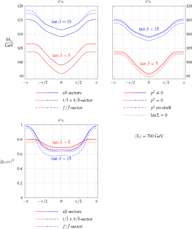
Figure 4: $M_{h_{1}}$ and $|g_{h_{1}VV}|^{2}$ are shown as a function of $\varphi_{X_{t}}$ for $|X_{t}|=700\,\,\mathrm{GeV}$, $\tan\beta=5,15$ and the other parameters as given in Eq. (101).

4.2.2 Dependence on the gaugino phases

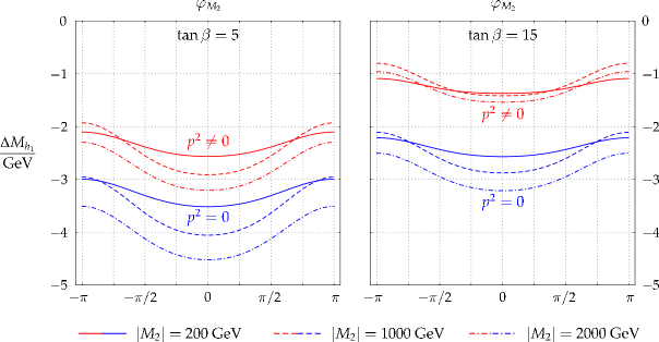
Figure 5: $\Delta M_{h_{1}}$ := $M_{h_{1}}$(all sectors) $-$ $M_{h_{1}}$($f/\tilde{f}$ sector) is shown as a function of $\varphi_{M_{2}}$ for the full result and the “$p^{2}=0$” approximation. The left plot shows the result for $\tan\beta=5$, while in the right plot $\tan\beta=15$. $|M_{2}|$ is chosen as $200,1000,2000\,\,\mathrm{GeV}$.

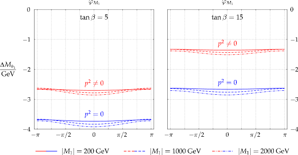
Figure 6: $\Delta M_{h_{1}}$ := $M_{h_{1}}$(all sectors) $-$ $M_{h_{1}}$($f/\tilde{f}$ sector) is shown as a function of $\varphi_{M_{1}}$ for the full result and the “$p^{2}=0$” approximation. The left plot shows the result for $\tan\beta=5$, while in the right plot $\tan\beta=15$. $|M_{1}|$ is chosen as $200,1000,2000\,\,\mathrm{GeV}$.

We now analyze the dependence on the gaugino phases $\varphi_{M_{1}}$ and $\varphi_{M_{2}}$. In Fig. 5 the dependence of the lightest cMSSM Higgs-boson mass on $\varphi_{M_{2}}$ is shown. The difference $\Delta M_{h_{1}}$ := $M_{h_{1}}$(all sectors) $-$ $M_{h_{1}}$($f/\tilde{f}$ sector), which is dominated by the chargino/neutralino contributions, is evaluated for three different values of $|M_{2}|$, $|M_{2}|=200,1000,2000\,\,\mathrm{GeV}$ (solid, dashed, dot-dashed line). The other parameters are chosen as in Eq. (101), and all other complex phases are set to zero. The result including the full momentum dependence is given by the upper set of curves, while the “$p^{2}=0$” approximation is given by the lower set. In the left plot we have chosen $\tan\beta=5$, in the right one $\tan\beta=15$. For the lower $\tan\beta$ value the effects from the non-sfermionic sector are about $2$–$3\,\,\mathrm{GeV}$ if the full dependence on the external momentum is taken into account, and about $4\,\,\mathrm{GeV}$ in the “$p^{2}=0$” approximation (which is used in the effective potential approach). The effect arising from varying the gaugino phase $\varphi_{M_{2}}$ itself is of ${\cal O}(1\,\,\mathrm{GeV})$. Both the overall effect from the non-sfermionic sector and the effect from varying $\varphi_{M_{2}}$ become smaller for larger $\tan\beta$ values (right plot). The effects are largest for $|M_{2}|=$${\cal O}(1\,\,\mathrm{TeV})$, i.e. for $|M_{2}|$ being of the same order as $|\mu|$. In this case the gaugino-higgsino mixing in the chargino and neutralino sector, and correspondingly the couplings of the charginos and neutralinos to the Higgs sector, is maximized. The effects shown in Fig. 5 arising from varying $\varphi_{M_{2}}$ should be interpreted as an upper bound on the possible impact of the phase dependence. The possible effects from the gaugino phases will be reduced if the existing experimental constraints on these phases are taken into account, see the discussion above.

We now turn to the effects from varying $\varphi_{M_{1}}$ as shown in Fig. 6. The parameters are as in Fig. 5, but with $M_{2}=500\,\,\mathrm{GeV}$ and $|M_{1}|=200,1000,2000\,\,\mathrm{GeV}$ (solid, dashed, dotted line). The size of the effects from the non-sfermion sector is the same as in Fig. 5. However, the dependence on $\varphi_{M_{1}}$ is much smaller, being of ${\cal O}(100\,\,\mathrm{MeV})$.

4.2.3 Decay widths of the neutral Higgs bosons

In this section we compare the predictions for the partial decay widths of all three neutral Higgs bosons to $\tau$ leptons based on the wave function normalization factors as given in Eqs. (88), (89) with the effective coupling approximation (using the “$p^{2}$ on-shell” approximation) according to Eqs. (94), (95), and with the “$p^{2}=0$” approximation as given in Eqs. (93), (94). In Fig. 7 we show

$$\Gamma_{i,\tau}:=\Gamma(h_{i}\to\tau^{+}\tau^{-})\mbox{~{}~{}and~{}~{}}\Gamma(h_{i}\to\tau^{+}\tau^{-})_{{\mathbf{R}}},\;\Gamma(h_{i}\to\tau^{+}\tau^{-})_{{\mathbf{U}}}$$ (102)

for $i=1,2,3$ (upper, middle, lower row), where $\Gamma$ refers to the full result based on the wave function normalization factors, and $\Gamma_{{\mathbf{U}}}$, $\Gamma_{{\mathbf{R}}}$ correspond to the effective coupling approximation evaluated with ${\mathbf{U}}_{\mathrm{n}}$ and ${\mathbf{R}}_{\mathrm{n}}$, respectively. Since we are only interested here in the comparison of the wave function normalization factors with the effective coupling approximations, we omit the contributions arising from the mixing of the physical Higgs states with the Goldstone boson and the $Z$ boson and we also do not take into account irreducible vertex corrections to the $h_{i}\tau^{+}\tau^{-}$ vertices. The results are shown for $M_{H^{\pm}}=150\,\,\mathrm{GeV}$ and $|X_{t}|=700\,\,\mathrm{GeV}$ as a function of $\varphi_{X_{t}}$, where the other parameters are chosen according to Eq. (101) with $\tan\beta=5$ (left) and $\tan\beta=15$ (right). As a general feature it can be observed that $\Gamma_{{\mathbf{U}}}$ is closer to the full result $\Gamma$ than $\Gamma_{{\mathbf{R}}}$ with only few exceptions (due to accidental numerical cancellations). This shows that the effective coupling defined through ${\mathbf{U}}_{\mathrm{n}}$, Eq. (95), gives a somewhat better numerical description than the one defined through ${\mathbf{R}}_{\mathrm{n}}$, Eq. (94), as used in the effective potential approach. For $\tan\beta=5$ the deviations between the “$p^{2}=0$” approximation and the full result are mostly at or below the 5% level, where the largest effects in general occur in the decay width of the lightest Higgs boson. For $\tan\beta=15$ the absolute and relative deviations between the effective coupling approximation and the full result can be significantly larger in the case of the lightest Higgs boson. For the decay widths of $h_{1}$ the full result can differ from the “$p^{2}=0$” approximation by more than 10%. In particular, in the region where $\Gamma(h_{1}\to\tau^{+}\tau^{-})$ has a minimum ($\varphi_{X_{t}}\approx\pm\pi$) the relative deviation between the full result and $\Gamma_{{\mathbf{R}}}$ reaches more than 25%. Also in this case the deviation between the full result and $\Gamma_{{\mathbf{U}}}$, based on the “$p^{2}$ on-shell” approximation, is much smaller. The deviations for $h_{2}$ and $h_{3}$ are again at the level of 5%. For larger values of $|X_{t}|$ even larger differences between the effective coupling approximation and the full result can be found.

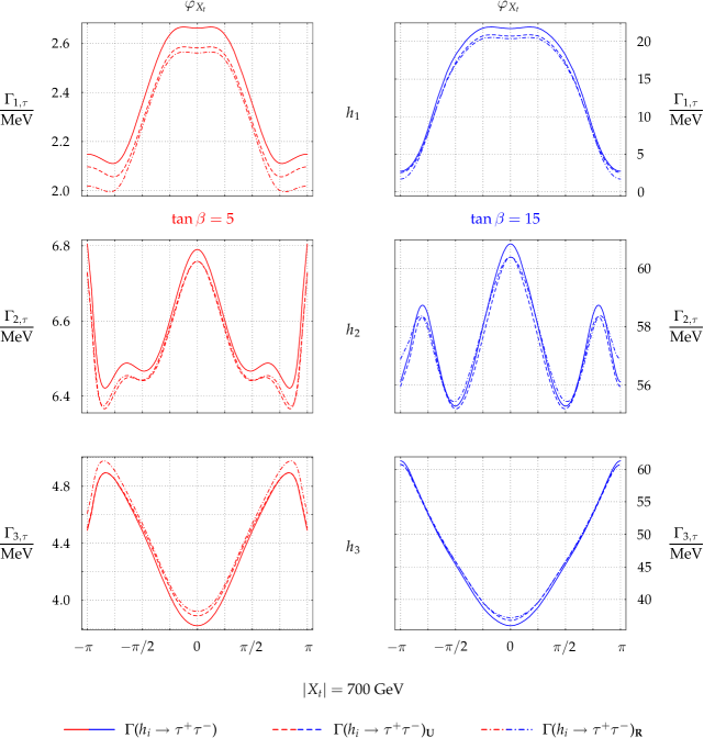
Figure 7: The decay widths $\Gamma(h_{i}\to\tau^{+}\tau^{-})$, $\Gamma(h_{i}\to\tau^{+}\tau^{-})_{{\mathbf{U}}}$ and $\Gamma(h_{i}\to\tau^{+}\tau^{-})_{{\mathbf{R}}}$ (see text) are shown for $i=1,2,3$ (upper, middle, lower row) as a function of $\varphi_{X_{t}}$ with $|X_{t}|=700\,\,\mathrm{GeV}$. In the left column $\tan\beta=5$, while for the plots in the right column $\tan\beta=15$. The other parameters are chosen according to Eq. (101).

4.3 Mass difference and mixing of the heavy neutral Higgs bosons

We now turn to the predictions for the masses and the mixing of the heavy neutral Higgs bosons of the cMSSM. The discovery of heavy Higgs bosons (in addition to a light one) would clearly establish an enlarged Higgs sector as compared to the SM. In the cMSSM the two heavy neutral Higgs bosons $h_{2}$ and $h_{3}$ are in general relatively close in mass, so that the mixing induced by the ${\cal CP}$-violating phases can give rise to resonance-type effects. We first analyze the mass difference of the two heavy neutral Higgs bosons, $\Delta M_{32}:=M_{h_{3}}-M_{h_{2}}$, in scenarios where the Higgs-boson self-energies can be enhanced by threshold effects. We then investigate the phase dependence of $\Delta M_{32}$ and discuss in how far this observable can be employed for distinguishing the cMSSM from the rMSSM. Finally we perform a detailed analysis of the mixing of $h_{2}$ and $h_{3}$ that is induced by the presence of complex phases.

4.3.1 Threshold effects for heavy Higgs bosons

We first analyze the effects of thresholds appearing in the Higgs-boson self-energy diagrams (e.g. for $m_{A}=m_{\tilde{t}_{1}}+m_{\tilde{t}_{2}}$, see the sixth diagram in Fig. 1) on the masses of the heavy neutral Higgs bosons. In the first two lines of Fig. 8 the mass difference $\Delta M_{32}:=M_{h_{3}}-M_{h_{2}}$ is shown as a function of $M_{H^{\pm}}$ for $\tan\beta=5$ (left) and $\tan\beta=15$ (right) for two different values of the phase of $A_{t}$, $\varphi_{A_{t}}=0$ (upper row) and $\varphi_{A_{t}}=\pi/2$ (middle row). The other parameters are chosen as in Eq. (101). We compare the full result (solid lines) with the “$p^{2}$ on-shell” (dot-dashed), “$p^{2}=0$” (dashed) and “$\mathop{\mathrm{Im}}\Sigma=0$” (dotted) approximations defined in Eqs. (79)–(81). It can be seen for the full result that the threshold effects may lead to a significant enhancement of the mass splitting between the states $h_{2}$ and $h_{3}$, so that mass differences in excess of $\Delta M_{32}=10\,\,\mathrm{GeV}$ can occur even for $M_{H^{\pm}}$ values in the decoupling region where $M_{H^{\pm}}\gg M_{Z}$. This behaviour is not reproduced in the “$p^{2}=0$” approximation (which is used in the effective potential approach). On the other hand, it turns out that the “$p^{2}$ on-shell” approximation, see Eq. (79), gives a rather good approximation to the full result. The remaining deviations stay below the level of $1\,\,\mathrm{GeV}$. It should be noted in this context that the sharp peaks displayed in Fig. 8 would get smoothened if the effects of finite widths of the internal particles in the Higgs-boson self-energies were taken into account. A precise prediction directly at threshold would require a dedicated analysis that is beyond the scope of the present paper.

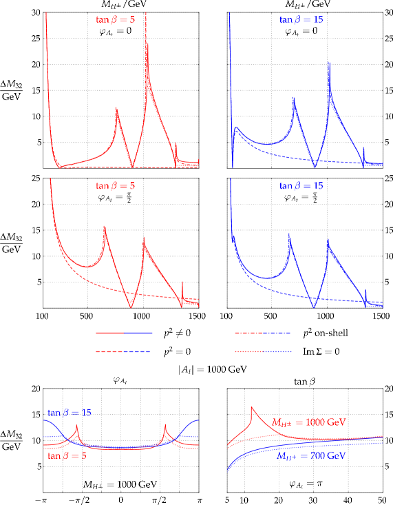
Figure 8: The mass difference $\Delta M_{32}:=M_{h_{3}}-M_{h_{2}}$ is shown as a function of $M_{H^{\pm}}$ (upper and middle rows) and as a function of $\varphi_{A_{t}}$ and $\tan\beta$ (lower row) for the parameters given in Eq. (101). The upper row shows the results for $\varphi_{A_{t}}=0$ with $\tan\beta=5$ (left) and $\tan\beta=15$ (right). The middle row shows $\Delta M_{32}$ for $\varphi_{A_{t}}=\pi/2$ with $\tan\beta=5$ (left) and $\tan\beta=15$ (right). The lower row shows $\Delta M_{32}$ for $\tan\beta=5,15$ and $M_{H^{\pm}}=1000\,\,\mathrm{GeV}$ as a function of $\varphi_{A_{t}}$ (left) and for $\varphi_{A_{t}}=\pi$, $M_{H^{\pm}}=700,1000\,\,\mathrm{GeV}$ as a function of $\tan\beta$ (right).

We now turn to the effects of the imaginary parts of the Higgs-boson self-energies, i.e. the comparison of the full result with the “$\mathop{\mathrm{Im}}\Sigma=0$” approximation as defined in Eq. (81). While for the example of the lightest cMSSM Higgs boson, shown in Fig. 4, the result for neglected imaginary parts was indistinguishable from the full result, for the mass difference of the heavy Higgs bosons a difference becomes visible in the two upper lines of Fig. 8 around the thresholds. The effect is shown in more detail in the lower line of Fig. 8. In the lower left plot we show $\Delta M_{32}$ as a function of $\varphi_{A_{t}}$ for $\tan\beta=5,15$ and $M_{H^{\pm}}=1000\,\,\mathrm{GeV}$. In the right plot we display $\Delta M_{32}$ as a function of $\tan\beta$ for $M_{H^{\pm}}=700,1000\,\,\mathrm{GeV}$ and $\varphi_{A_{t}}=\pi$. The other parameters are again those of Eq. (101). As one can see from the plot, the difference between the full result and the approximation with neglected imaginary parts can be as large as about $5\,\,\mathrm{GeV}$.

4.3.2 Phase dependence of $\Delta M_{32}$

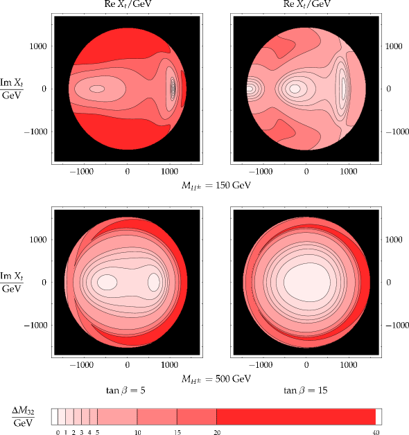
Figure 9: $\Delta M_{32}:=M_{h_{3}}-M_{h_{2}}$ is shown in the $\mathop{\mathrm{Re}}X_{t}$–$\mathop{\mathrm{Im}}X_{t}$ plane for $\tan\beta=5$ (left) and $\tan\beta=15$ (right) for $M_{H^{\pm}}=150\,\,\mathrm{GeV}$ (upper row) and $M_{H^{\pm}}=500\,\,\mathrm{GeV}$ (lower row). The other parameters are as given in Eq. (101).

We now analyze the dependence of the mass difference $\Delta M_{32}:=M_{h_{3}}-M_{h_{2}}$ on the complex phases in more detail, in particular in view of the question whether the detection of a certain mass difference between the two heavy neutral Higgs bosons could be a direct indication of non-zero complex phases in the MSSM. In Fig. 9 we show $\Delta M_{32}$ in the $\mathop{\mathrm{Re}}X_{t}$–$\mathop{\mathrm{Im}}X_{t}$ plane for $\tan\beta=5$ (left) and $\tan\beta=15$ (right) for $M_{H^{\pm}}=150\,\,\mathrm{GeV}$ (upper row) and $M_{H^{\pm}}=500\,\,\mathrm{GeV}$ (lower row). The other parameters are given in Eq. (101).

The results in Fig. 9 show that the smallest mass differences between $M_{h_{3}}$ and $M_{h_{2}}$ occur if $X_{t}\equiv A_{t}-\mu/\tan\beta$ is real or has only a relatively small imaginary part. For $M_{H^{\pm}}=150\,\,\mathrm{GeV}$ and low $\tan\beta$ this happens only around $X_{t}\approx 1000\,\,\mathrm{GeV}$, while for higher $\tan\beta$ three minima are reached for $X_{t}\approx-1200,-200,800\,\,\mathrm{GeV}$. The largest mass differences are realized for relatively large $|X_{t}|$. While for $\tan\beta=5$ all possible mass differences occurring in the $\mathop{\mathrm{Re}}X_{t}$–$\mathop{\mathrm{Im}}X_{t}$ plane are also realized on the real axis, for $\tan\beta=15$ the largest mass differences can only be found for a non-zero imaginary part of $X_{t}$.

The qualitative behaviour changes somewhat for $M_{H^{\pm}}=500\,\,\mathrm{GeV}$. Again the smallest mass differences between $M_{h_{3}}$ and $M_{h_{2}}$ occur for small imaginary parts of $X_{t}$. Two minima are found for $\tan\beta=5$. On the other hand, for $\tan\beta=15$ only the region of the $\mathop{\mathrm{Re}}X_{t}$–$\mathop{\mathrm{Im}}X_{t}$ parameter space around $X_{t}=0$ results in a small value of $\Delta M_{32}$. The rather symmetric shape of the plot for $\tan\beta=15$ and $M_{H^{\pm}}=500\,\,\mathrm{GeV}$ around $X_{t}=0$ shows that in this case the dominant contribution to $\Delta M_{32}$ depends only on the absolute value $|X_{t}|\approx|A_{t}|$. For $\tan\beta=5$, on the other hand, the minimum values of $\Delta M_{32}$ are reached for both $\mathop{\mathrm{Re}}A_{t}\neq 0$ and $\mathop{\mathrm{Re}}X_{t}\neq 0$. Similarly to the case of $M_{H^{\pm}}=150\,\,\mathrm{GeV}$ and low $\tan\beta$ we find also for $M_{H^{\pm}}=500\,\,\mathrm{GeV}$ (both for low and high $\tan\beta$) that a large mass difference $\Delta M_{32}$ does not necessarily require a non-zero complex phase of $X_{t}$. Indeed, for large $M_{H^{\pm}}$ all mass differences realized for a parameter point in the complex $X_{t}$ plane are also realized on its real axis. This means that the determination of the mass difference $\Delta M_{32}$ alone will in general not be sufficient to obtain direct information about the size of the complex phases. On the other hand, the interpretation of an observed mass difference in terms of the underlying SUSY parameters will be different in the rMSSM and the cMSSM. Valuable information for determining the parameters of the cMSSM including their complex phases can therefore be obtained by combining the mass difference $\Delta M_{32}$ with a suitable set of observables that exhibit a non-trivial dependence on the complex phases.

We have investigated also the effects of the complex phases of $M_{2}$ and $M_{1}$ on the mass difference $\Delta M_{32}$. The effects stay below the $1\,\,\mathrm{GeV}$ level for most parts of the parameter space.

4.3.3 Mixing of the heavy neutral Higgs bosons

We finally analyze the mixing of the two heavy neutral Higgs bosons. Mixing effects, especially between the second and the third Higgs boson, can potentially be sizable in the cMSSM. In Ref. [54] it was argued that the phases of the gaugino mass parameters play an important role in this context.

As explained above, the elements of ${\mathbf{U}}_{\mathrm{n}}$ (or ${\mathbf{R}}_{\mathrm{n}}$) can be used to quantify the extent of ${\cal CP}$-violation. For example, the combination $U_{31}^{2}+U_{32}^{2}$ can be understood as the ${\cal CP}$-even part in $h_{3}$, while the component $U_{33}^{2}$ corresponds to the ${\cal CP}$-odd part. The unitarity of ${\mathbf{U}}_{\mathrm{n}}$ ensures that both parts add up to 1.

We first discuss the ${\cal CP}$-conserving case, where $U_{33}^{2}$ is either 1 or 0, depending on the mass ordering of $M_{H}$ and $M_{A}$ (the higher-order corrected masses of the heavy neutral ${\cal CP}$ eigenstates). In Fig. 10 we show the mass difference $\Delta M_{32}=M_{h_{3}}-M_{h_{2}}=|M_{H}-M_{A}|$ together with the effective couplings $U_{33}^{2}$ (based on the “$p^{2}$ on-shell” approximation, see Eq. (95)) and $R_{33}^{2}$ (obtained in the “$p^{2}=0$” approximation, see Eq. (94)). The three quantities are given as a function of $X_{t}$, which in the ${\cal CP}$-conserving case is a real parameter. We have set $M_{H^{\pm}}=500\,\,\mathrm{GeV}$, $\tan\beta=5$ ($\tan\beta=15$) in the left (right) plot, and the other parameters are chosen according to Eq. (101). The change from 1 to 0 in the $(33)$ element of the rotation matrix should obviously occur at the same value of $X_{t}$ where the mass hierarchy of the states $H$ and $A$ is inverted, i.e. where $\Delta M_{32}=0$. This correlation between the masses and the effective couplings is not automatic, however, since the masses have been calculated using the full higher-order corrections, while as discussed in Sect. 3.6 the effective couplings can only be obtained using certain approximations. Fig. 10 shows that the behaviour of $U_{33}^{2}$ with $X_{t}$ is well matched to the one of $\Delta M_{32}$, i.e. the step in $U_{33}^{2}$ occurs very close to the $X_{t}$ value where $\Delta M_{32}=0$. For $R_{33}^{2}$, on the other hand, the behaviour of the effective coupling significantly differs from the one of the higher-order corrected masses. This effect is particularly pronounced for small $\tan\beta$ as can be seen in the left plot, where the value of $X_{t}$ for which $\Delta M_{32}\approx 0$ is reached differs by more than $100\,\,\mathrm{GeV}$ from the corresponding $X_{t}$ value for which $R_{33}^{2}$ changes from 0 to 1. For $\tan\beta=15$ (right plot) the deviation is smaller but still significant. Fig. 10 clearly shows that those contributions which are omitted if effective couplings are constructed using the “$p^{2}=0$” approximation (as done in the effective potential approach) can be numerically sizable and important for a physically well-behaved result. We find also in this case (for not too large values of $M_{H^{\pm}}$) that a better numerical description is obtained with effective couplings defined through ${\mathbf{U}}_{\mathrm{n}}$, Eq. (95). At large $M_{H^{\pm}}$ values both matrices are insufficient for a precise description.

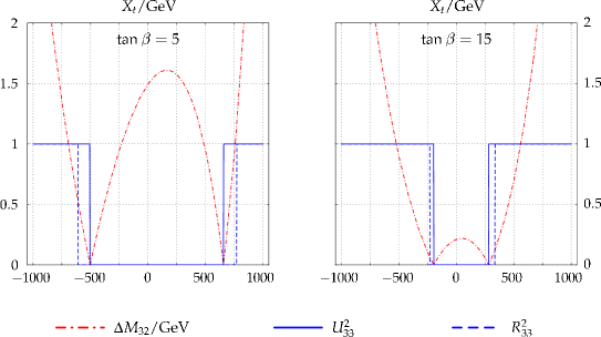
Figure 10: The mass difference $\Delta M_{32}=|M_{H}-M_{A}|$ and the effective couplings $U_{33}^{2}$ and $R_{33}^{2}$ (based on the “$p^{2}$ on-shell” and “$p^{2}=0$” approximations, respectively) are shown as a function of $X_{t}$ (chosen to be real) for $M_{H^{\pm}}=500\,\,\mathrm{GeV}$, $\tan\beta=5$ (left) and $\tan\beta=15$ (right). The other parameters are chosen according to Eq. (101).

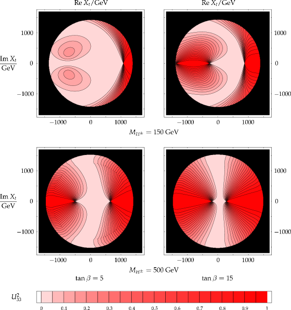
Figure 11: $U_{33}^{2}$ is shown in the $\mathop{\mathrm{Re}}X_{t}$–$\mathop{\mathrm{Im}}X_{t}$ plane for $\tan\beta=5$ (left) and $\tan\beta=15$ (right) for $M_{H^{\pm}}=150\,\,\mathrm{GeV}$ (upper row) and $M_{H^{\pm}}=500\,\,\mathrm{GeV}$ (lower row). The other parameters are as given in Eq. (101).

Now we focus on the mixing of the heavy neutral Higgs bosons in the presence of complex parameters. As a measure of the mixing between these two states we show in Fig. 11 $U_{33}^{2}$ in the $\mathop{\mathrm{Re}}X_{t}$–$\mathop{\mathrm{Im}}X_{t}$ plane. The choice for $M_{H^{\pm}}$ and $\tan\beta$ is the same as in Fig. 9, and the other parameters are specified in Eq. (101). We have checked that $U_{13}^{2}$ is very close to zero (i.e. the lightest Higgs boson is nearly a pure ${\cal CP}$-even state) and $U_{33}^{2}\approx 1-U_{23}^{2}$. The mixing varies strongly with $\varphi_{X_{t}}$ for both values of $\tan\beta$ and low and high $M_{H^{\pm}}$. In particular, for relatively large values of $|X_{t}|$, the variation of the phase $\varphi_{X_{t}}$ (with $|X_{t}|$ kept fixed) can cause $U_{33}^{2}$ (and consequently also $U_{23}^{2}$) to take on any value in the range $0\leq U_{33}^{2}\leq 1$. It can furthermore be seen in all four panels of Fig. 11 that a large mixing between the two heavy neutral Higgs bosons, corresponding to the parameter regions where $U_{33}^{2}\sim 0.5$, is a feature that can happen quite easily in the MSSM with complex parameters. Studying the properties of the heavy Higgs bosons is therefore of particular interest, since they could, at least in principle, give access to large ${\cal CP}$-violating effects.

The connection between $\Delta M_{32}$ (the mass difference between the two heavy Higgs bosons) and $U_{33}^{2}$ (the mixing of $h_{2}$ and $h_{3}$, i.e. the ${\cal CP}$ composition of the two heavy Higgs bosons) can be analyzed by comparing Fig. 11 with Fig. 9 (the choice for $M_{H^{\pm}}$ and $\tan\beta$ is the same in both figures). The regions of the nodal points in Fig. 11, i.e. the points in which a change in $X_{t}$ causes the largest variation in $U_{33}^{2}$, coincide with the regions where the mass difference $\Delta M_{32}$ is close to zero. This behaviour, which occurs for all $M_{H^{\pm}}$ and $\tan\beta$ values, is clearly a resonance-type effect: in the parameter regions where the masses of the Higgs states become degenerate, the mixing effects between the states are maximal.

Finally we analyze the effect of the gaugino phases on the mixing of the heavy neutral Higgs bosons. The dependence of $U_{33}^{2}$ on the gaugino phases is depicted in Fig. 12 for $\tan\beta=5$ and $M_{H^{\pm}}=500\,\,\mathrm{GeV}$. We have chosen $\mathop{\mathrm{Re}}X_{t}$ as $\mathop{\mathrm{Re}}X_{t}=655\,\,\mathrm{GeV}$ such that $\mathop{\mathrm{Im}}X_{t}=0$ corresponds to a resonance region where $\Delta M_{32}$ is close to zero, namely the right nodal point in the lower left plot of Fig. 11. For displaying the effects of the gaugino phases $\varphi_{M_{2}}$ and $\varphi_{M_{1}}$ we have chosen in Fig. 12 three different values of the imaginary part of $X_{t}$, $\mathop{\mathrm{Im}}X_{t}=0,20,200\,\,\mathrm{GeV}$ (solid, dashed, dot-dashed lines). For the case of the nodal point where $\mathop{\mathrm{Im}}X_{t}=0$ a very strong variation of $U_{33}^{2}$ with both $\varphi_{M_{2}}$ (left plot) and $\varphi_{M_{1}}$ (right plot) is observed, covering the whole allowed range $0\leq U_{33}^{2}\leq 1$. It should be noted that one encounters in this case a strong variation of $U_{33}^{2}$ with the gaugino phases even if $\varphi_{M_{2}}$, $\varphi_{M_{1}}$ are restricted to relatively small values. However, for $\mathop{\mathrm{Im}}X_{t}=20\,\,\mathrm{GeV}$, i.e. only slightly away from the nodal point, the dependence of $U_{33}^{2}$ on the gaugino phases is already much smaller. For $\mathop{\mathrm{Im}}X_{t}=200\,\,\mathrm{GeV}$ the variation of $U_{33}^{2}$ with $\varphi_{M_{2}}$ and $\varphi_{M_{1}}$ is numerically insignificant. It becomes apparent that the gaugino phases can have a strong impact on the mixing of the heavy Higgs bosons, but only directly on resonance. Outside of the resonance regions the effects of the gaugino phases are small. This is in contrast to Ref. [54], where it was claimed that a strong dependence of the Higgs mixing on $\varphi_{M_{2}}$ and $\varphi_{M_{1}}$ were a general feature of the cMSSM.

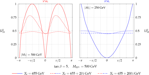
Figure 12: $U_{33}^{2}$ is shown as a function of $\varphi_{M_{2}}$ (left plot) and $\varphi_{M_{1}}$ (right plot) for $\mathop{\mathrm{Re}}X_{t}=655\,\,\mathrm{GeV}$ and $\mathop{\mathrm{Im}}X_{t}=0,20,200\,\,\mathrm{GeV}$ (solid, dashed, dot-dashed lines). The other parameters are the same as in Fig. 11.

5 The code FeynHiggs 2.5: program features

FeynHiggs 2.5 [23, 44, 45, 46] is a Fortran code for the evaluation of the masses, decays and production processes of Higgs bosons in the MSSM with real or complex parameters. In this section we give a short overview about its features. More detailed information about installation and use can be found in the Appendix.

The calculation of the higher-order corrections is based on the Feynman-diagrammatic (FD) approach as outlined in the previous sections. At the one-loop level, it consists of a complete evaluation, including the full momentum and phase dependence, and as a further option the full $6\times 6$ non-minimal flavor violation (NMFV) contributions for scalar quarks [95, 96]. At the two-loop level all available corrections from the real MSSM have been included (see Refs. [41, 97, 98] for reviews). They are supplemented by the resummation of the leading effects from the (scalar) $b$ sector including the full complex phase dependence [99].

The loop-corrected pole masses are determined as the real parts of the complex poles as described in Sect. 3.4. The imaginary parts of the Higgs-boson self-energies are fully taken into account. The masses are evaluated with two independent numerical algorithms. Deviations between the two methods indicate potential problems of numerical stability. In addition to the Higgs-boson masses, the program also provides results for the effective Higgs-boson couplings and the wave function normalization factors for external Higgs bosons as described in Sects. 3.5,3.6.

Besides the computation of the Higgs-boson masses, effective couplings and wave function normalization factors, the program also evaluates an estimate for the theory uncertainties of these quantities due to unknown higher-order corrections. The total uncertainty is the sum of deviations from the central value, $\Delta X=\sum_{i=1}^{3}|X_{i}-X|$ with $X=\{M_{h_{1},h_{2},h_{3},H^{\pm}},U_{ij},Z_{ij}\}$, where $U_{ij}$ is defined in Eq. (95) and $Z_{ij}$ in Eqs. (88)–(89). Alternatively instead of $U_{ij}$ also $R_{ij}$, defined in Eq. (94), can be evaluated. The $X_{i}$ are given by

• $X_{1}$ is obtained by varying the renormalization scale (entering via the $\overline{\text{DR}}$ renormalization) within $\frac{1}{2}m_{t}\leqslant\mu\leqslant 2m_{t}$,

• $X_{2}$ is obtained by using $m_{t}^{\text{pole}}$ instead of the running $m_{t}$ in the two-loop corrections,

• $X_{3}$ is obtained by using an unresummed bottom Yukawa coupling, $y_{b}$, i.e. a $y_{b}$ including the leading ${\cal O}(\alpha_{s}\alpha_{b})$ corrections, but not resummed to all orders.

Furthermore FeynHiggs 2.5 contains the evaluation of all relevant Higgs-boson decay widths and effective couplings (the latter are given in the conventions used in the MSSM model file of the program FeynArts [70]). In particular, the following quantities are calculated:

• the total width for the neutral and charged Higgs bosons,

• the branching ratios and effective couplings of the three neutral Higgs bosons to

  • SM fermions (see also Refs. [50, 97]), $h_{i}\to\bar{f}f$,

  • SM gauge bosons (possibly off-shell), $h_{i}\to\gamma\gamma,ZZ^{*},WW^{*},gg$,

  • gauge and Higgs bosons, $h_{i}\to Zh_{j}$, $h_{i}\to h_{j}h_{k}$,

  • scalar fermions, $h_{i}\to\tilde{f}^{\dagger}\tilde{f}$,

  • gauginos, $h_{i}\to\tilde{\chi}^{\pm}_{k}\tilde{\chi}^{\mp}_{j}$, $h_{i}\to\tilde{\chi}^{0}_{l}\tilde{\chi}^{0}_{m}$,

• the branching ratios and effective couplings of the charged Higgs boson to

  • SM fermions, $H^{-}\to\bar{f}f^{\prime}$,

  • a gauge and Higgs boson, $H^{-}\to h_{i}W^{-}$,

  • scalar fermions, $H^{-}\to\tilde{f}^{\dagger}\tilde{f}^{\prime}$,

  • gauginos, $H^{-}\to\tilde{\chi}^{-}_{k}\tilde{\chi}^{0}_{l}$.

• the production cross sections of the neutral Higgs bosons at the Tevatron and the LHC in the approximation where the corresponding SM cross section is rescaled by the ratios of the corresponding partial widths in the MSSM and the SM or by the wave function normalization factors for external Higgs bosons as defined through Eqs. (88)–(89), see Ref. [100] for further details.

For comparisons with the SM, the following quantities are also evaluated for SM Higgs bosons with the same mass as the three neutral MSSM Higgs bosons:

• the total decay width,

• the couplings and branching ratios of a SM Higgs boson to SM fermions,

• the couplings and branching ratios of a SM Higgs boson to SM gauge bosons (possibly off-shell).

• the production cross sections at the Tevatron and the LHC [100].

FeynHiggs 2.5 furthermore provides results for electroweak precision observables that give rise to constraints on the SUSY parameter space (see Ref. [42] and references therein):

• the quantity $\Delta\rho$ up to the two-loop level [101] that can be used to indicate disfavored scalar top and bottom mass combinations,

• an evaluation of $M_{W}$ and $\sin^{2}\theta_{\mathrm{eff}}$, where the SUSY contributions are treated in the $\Delta\rho$ approximation (see e.g. Ref. [42]), taking into account at the one-loop level the effects of complex phases in the scalar top/bottom sector [102] as well as NMFV effects [95],

• the anomalous magnetic moment of the muon, including a full one-loop calculation [103, 104] as well as leading and subleading two-loop corrections [106, 105] (see also Ref. [107]),

• the evaluation of ${\rm BR}(b\to s\gamma)$ including NMFV effects [96].

Finally, FeynHiggs 2.5 possesses some further features:

• Transformation of the input parameters from the $\overline{\rm{DR}}$ to the on-shell scheme (for the scalar top and bottom parameters), including the full ${\cal O}(\alpha_{s})$ and ${\cal O}(\alpha_{t,b})$ corrections.

• Processing of SUSY Les Houches Accord (SLHA 2) data [108, 109, 110]. FeynHiggs 2.5 reads the output of a spectrum generator file and evaluates the Higgs boson masses, branching ratios etc. The results are written in the SLHA format to a new output file.

• Predefined input files for the SPS benchmark scenarios [111] and the Les Houches benchmarks for Higgs boson searches at hadron colliders [112] are included.

• Detailed information about all the features of FeynHiggs 2.5 are provided in man pages.

6 Conclusions

We have presented new results for the complete one-loop contributions to the masses and mixing effects in the Higgs-boson sector of the MSSM with complex parameters. They have been obtained in the Feynman-diagrammatic approach using a hybrid renormalization scheme where the masses are renormalized on-shell, while the $\overline{\rm{DR}}$ scheme is applied for $\tan\beta$ and the field renormalizations. A detailed description has been given of the renormalization procedure and of the determination of the masses as the real parts of the complex poles of the higher-order corrected Higgs propagator matrix. Besides the Higgs-boson masses we have also derived the wave function normalization factors needed for processes with external Higgs bosons. We have discussed different ways for defining effective Higgs-boson couplings that incorporate leading higher-order effects. As a result, we propose effective couplings based on the “$p^{2}$ on-shell” approximation, where the Higgs-boson self-energies are evaluated at the tree-level masses.

In our calculation of the Higgs-boson masses, couplings and wave function normalizations the full dependence on all relevant complex phases is taken into account. We incorporate for the first time the complete effects arising from the imaginary parts of the one-loop Higgs-boson self-energies in a consistent way. Our result for the complete one-loop contributions in the cMSSM is supplemented by all available two-loop corrections in the rMSSM and a resummation of the leading effects from the sbottom sector for complex parameters.

In our numerical discussion we have first analyzed the impact of our results on the physics of the light Higgs boson, which is of interest in view of the current exclusion bounds and possible high-precision measurements of the properties of a light Higgs boson at the next generation of colliders. We first investigated the impact of the different MSSM sectors and the possible effects of the corresponding complex phases on the mass of the lightest neutral Higgs boson of the cMSSM Higgs, $M_{h_{1}}$, and the coupling of the lightest Higgs to gauge bosons. The well-known result from the rMSSM that the bulk of the corrections to $M_{h_{1}}$ arises from the fermion/sfermion sector is of course also reflected in the dependence on the associated complex phases. We find that the effects associated with the variation of $\varphi_{X_{t}}$ are in general numerically very important, leading to shifts in $M_{h_{1}}$ of up to $8\,\,\mathrm{GeV}$ in the examples that we have studied. The corrections beyond the fermion/sfermion loops, arising from the chargino/neutralino sector, the gauge-boson sector and the Higgs sector, can amount up to about $3\,\,\mathrm{GeV}$. The dependence of $M_{h_{1}}$ on the gaugino phases $\varphi_{M_{2}}$ and $\varphi_{M_{1}}$ is in general rather small and will be difficult to resolve even in the high-precision environment of the ILC (in particular in view of the existing experimental constraints on the gaugino phases).

We have furthermore compared our full result with various aproximations. We find sizable deviations of up to $1.5\,\,\mathrm{GeV}$ in $M_{h_{1}}$ between the full result and the “$p^{2}=0$” approximation, which is often used in the literature. We find that the “$p^{2}$ on-shell” approximation is significantly closer to the full result with maximum deviations below $0.5\,\,\mathrm{GeV}$.

For the example of the partial decay widths of the three neutral Higgs bosons into $\tau$ leptons we have compared the results based on the wave function normalization factors of the external Higgs bosons with effective-coupling approximations. The dependence of the partial widths on the phase $\varphi_{X_{t}}$ is very pronounced. We find that the result based on an effective coupling in the “$p^{2}=0$” approximation (corresponding to the effective potential approach) deviates from the full result by typically up to 5%, with maximum deviations of more than 10%. The effective couplings in the “$p^{2}$ on-shell” approximation show a better agreement with the full result for not too large values of $M_{H^{\pm}}$.

While over a large part of the cMSSM parameter space the lightest neutral Higgs boson is almost a pure ${\cal CP}$-even state, large ${\cal CP}$-violating effects may influence the masses and mixings of the two heavier neutral Higgs bosons of the cMSSM. We have analyzed the impact of complex phases on the mass difference between the two heavy Higgs bosons, $\Delta M_{32}$, and on their mixing properties. Our full result has been compared with various approximations. We find that the mass difference $\Delta M_{32}$ can significantly be enhanced by threshold effects, so that mass differences of more than $10\,\,\mathrm{GeV}$ are possible even in the decoupling region where $M_{H^{\pm}}\gg M_{Z}$. Since the threshold effects go beyond the “$p^{2}=0$” approximation, large deviations between the full result and this approximation may occur. The “$p^{2}$ on-shell” approximation, on the other hand, is close to the full result even in the threshold region. We have furthermore shown that effects of the imaginary parts of the Higgs-boson self-energies can be sizable in the threshold region. They can be as large as about $5\,\,\mathrm{GeV}$ in this region.

While the mass difference $\Delta M_{32}$ is sensitive to the effects of the complex phases in the sfermion sector (the effects of the gaugino phases, on the other hand, are small), a determination of $\Delta M_{32}$ will in general not be sufficient to establish the existence of non-zero complex phases. We have shown that most values of $\Delta M_{32}$ that can be obtained in the complex $\mathop{\mathrm{Re}}X_{t}$–$\mathop{\mathrm{Im}}X_{t}$ plane can also be realized on the real axis, i.e. for $\mathop{\mathrm{Im}}X_{t}=0$. In order to extract information on the complex phases, the mass difference $\Delta M_{32}$ will have to be combined with a suitable set of observables that exhibit a non-trivial dependence on the complex phases.

We find that a large (${\cal CP}$-violating) mixing between the two heavy Higgs states is possible over a significant part of the cMSSM parameter space. In the parameter regions where the mass difference $\Delta M_{32}$ becomes very small a resonance-type behaviour is possible. It gives rise to large variations in the mixing between the two Higgs bosons, i.e. a small change in the phase $\varphi_{X_{t}}$ can have a dramatic effect on the mixing properties. Directly on resonance even the gaugino phases $\varphi_{M_{2}}$ and $\varphi_{M_{1}}$ have a large impact on the Higgs mixing. In contrast to Ref. [54], where it was claimed that a strong dependence of the Higgs mixing on $\varphi_{M_{2}}$ and $\varphi_{M_{1}}$ were a general feature of the cMSSM, we find that outside of the resonance regions the effects of the gaugino phases are small. For a reliable description of the resonance region it is crucial to correctly take into account the imaginary parts of the Higgs-boson self-energies.

Our analysis has shown that effective couplings in the “$p^{2}=0$” approximation, as used in the effective potential approach, can be insufficient for correctly matching the Higgs-mixing properties to the higher-order corrected Higgs-boson masses. The effective couplings based on the “$p^{2}$ on-shell” approximation that we have studied in this paper, on the other hand, have turned out to be well-suited for a numerical description of the Higgs-boson mixing for not too large values of $M_{H^{\pm}}$. However, for large $M_{H^{\pm}}$ the correct decoupling properties of the effective couplings of the lightest Higgs boson are achieved in the “$p^{2}=0$” approximation, but not in the “$p^{2}$ on-shell” approximation.

Our results for the Higgs-boson masses, couplings and wave function normalization factors together with an estimate of the remaining theoretical uncertainties from unknown higher-order corrections are implemented into the public Fortran code FeynHiggs 2.5. The code also contains the evaluation of the Higgs-boson decays and the main Higgs-boson production channels at the Tevatron and the LHC, calculated using the full wave function normalization factors. Further quantities that are useful for deriving constraints on the SUSY parameter space are also evaluated, such as electroweak precision observables, the anomalous magnetic moment of the muon and (in the case of complex parameters) electric dipole moments. The code can be obtained from www.feynhiggs.de .

Acknowledgements

We thank K. Williams for numerous checks and helpful discussions. We are grateful to D. Stöckinger for illuminating discussions, in particular on Ref. [78], and we also thank S. Hesselbach, C. Schappacher and P. Slavich for interesting discussions. W.H. wants to express special thanks to the Institute of Theoretical Physics, University of Vienna, where this paper was finalized while he was Erwin Schrödinger visiting professor.

Appendix A The code FeynHiggs 2.5: installation and use

A.1 Installation and Use

The installation process is straightforward and should take no more than a few minutes:

• Download the latest version from www.feynhiggs.de and unpack the tar archive.

• The package is built with ./configure and make. This creates the library libFH.a and the command-line frontend FeynHiggs.

• To build also the Mathematica frontend MFeynHiggs, invoke make all.

• make install installs the files into a platform-dependent directory tree, for example i586-linux/{bin,lib,include}.

• Finally, remove the intermediate files with make clean.

FeynHiggs 2.5 has four modes of operation,

• Library Mode: Invoke the FeynHiggs routines from a Fortran or C/C++ program linked against the libFH.a library.

• Command-line Mode: Process parameter files in native FeynHiggs or SLHA format at the shell prompt or in scripts with the standalone executable FeynHiggs.

• WWW Mode: Interactively choose the parameters at the FeynHiggs User Control Center (FHUCC) and obtain the results on-line.

• Mathematica Mode: Access the FeynHiggs routines in Mathematica via MathLink with MFeynHiggs.

A.1.1 Library Mode

The core functionality of FeynHiggs 2.5 is implemented in a static Fortran 77 library libFH.a. All other interfaces are ‘just’ frontends to this library.

In view of Fortran’s lack of symbol scoping, all internal symbols have been prefixed to make symbol collisions very unlikely. Also, the library contains only subroutines, no functions, which simplifies the invocation. In Fortran, no include files are needed except for access to the coupling structure. In C/C++, a single include file CFeynHiggs.h must be included once for the prototypes. Detailed debugging output can be turned on at run time.

The library provides the following functions:

• FHSetFlags sets the flags for the calculation.

• FHSetPara sets the input parameters directly, or
  FHSetSLHA sets the input parameters from SLHA data.

• FHSetCKM sets the elements of the CKM matrix.

• FHSetNMFV sets the off-diagonal soft SUSY-breaking parameters in the scalar quark sector that induce NMFV effects.

• FHSetDebug sets the debugging level.

• FHGetPara retrieves (some of) the MSSM parameters calculated from the input parameters, e.g. the sfermion masses.

• FHHiggsCorr computes the corrected Higgs masses, effective couplings and wave function normalization factors.

• FHUncertainties estimates the uncertainties of the Higgs masses, effective couplings and wave function normalization factors.

• FHCouplings computes the Higgs couplings and BRs.

• FHHiggsProd calculates the Higgs-boson production cross-sections at the Tevatron and the LHC.

• FHConstraints evaluates further electroweak precision observables.

These functions are described in detail in their respective man pages in the FeynHiggs package.

A.1.2 Command-line Mode

The FeynHiggs executable is a command-line frontend to the libFH.a library. It is invoked at the shell prompt as

   FeynHiggs inputfile [flags [scalefactor]]

where

• inputfile is the name of a parameter file (see below).

• flags is an (optional) string of integers giving the flag values, e.g. 40030211 (for details see the description of FHSetFlags in the man pages). If flags is not specified, 40020211 is used. The fifth flag controls the evaluation of the effective couplings, where 0 correspongs to the ”$p^{2}$ on-shell” and 4 to the ”$p^{2}=0$” approximation.

• scalefactor is an optional factor multiplying the renormalization scale. It is used to determine the dependence on the renormalization scale, e.g. by varying scalefactor from 0.5 to 2.

FeynHiggs understands two kinds of parameter files:

• Files in SUSY Les Houches Accord (SLHA) format. In this case FeynHiggs adds the Higgs masses, mixings and decay widths to the SLHA data structure and writes the latter to a file inputfile.fh.

  In fact, FeynHiggs tries to read each file in SLHA format first, and if that fails, falls back to its native format.

• Files in its native format, for example

    MT         171.4
    MB         4.7
    MW         80.392
    MZ         91.1875
    MSusy      500
    MA0        200
    Abs(M_2)   200
    Abs(MUE)   1000
    TB         5
    Abs(Xt)    1000
    Abs(M_3)   800
  

  The syntax should be pretty self-explanatory. Complex quantities can be given either in terms of absolute value Abs(X) and phase Arg(X), or as real part Re(X) and imaginary part Im(X). Abbreviations, summarizing several parameters (such as MSusy) can be used, or detailed information about the various soft SUSY-breaking parameters can be given.

  Furthermore, it is possible to define loops over parameters, to scan parts of parameter space. For example,

    TB         5 25 5
    MA0        100 800 *2
    MSusy      500 1000 /3
  

  declares three loops:
  a) over $\tan\beta$ from 5 to 25 linearly in steps of 5 (i.e. 5, 10, 15, 20, 25),
  b) over $M_{A}$ from 100 to 800 logarithmically in steps of 2 (i.e. 100, 200, 400, 800),
  c) over $M_{\rm SUSY}$ from 500 to 1000 linearly in 3 steps (i.e. 500, 750, 1000).

  The output is written in a human-readable form to the screen. Since this can be quite lengthy, a % is printed in front of all lines with ‘non-essential’ information, e.g. the details on couplings and decay widths. Thus to display only the ‘essential’ information, one just has to “grep” away the % lines, i.e.

    FeynHiggs inputfile flags | grep -v %
  

  The output can also be piped through the table filter to yield a machine-readable version appropriate for plotting etc. For example,

    FeynHiggs inputfile flags | table TB Mh0 > outputfile
  

  creates outputfile with two columns, $\tan\beta$ and $M_{h}$. The syntax of the output file is given as screen output.

Debugging output is governed by the environment variable FHDEBUG which can be set to an integer from 0 to 3 (for details see the description of FHSetDebug in the man pages). For example,

   setenv FHDEBUG 1     (in csh or tcsh)
   export FHDEBUG=1     (in sh or bash)

sets debugging level 1.

A.1.3 WWW Mode

The FeynHiggs User Control Center (FHUCC) is a WWW interface to the command-line executable FeynHiggs. It provides a convenient way to play with parameters, but is of course not suited for large-scale parameter scans or extensive analyses.

To use the FHUCC, point your favorite Web browser at

   http://www.feynhiggs.de/fhucc

adjust the parameters, and submit the form to see the results. At the end of the result page, the input file used for that FeynHiggs run is presented, too.

A.1.4 Mathematica Mode

The MFeynHiggs executable provides access to the FeynHiggs functions from Mathematica via the MathLink protocol. This is particularly convenient both because FeynHiggs can be used interactively this way and because Mathematica’s sophisticated numerical and graphical tools, e.g. FindMinimum, are available.

After starting Mathematica, install the package with

   In[1]:= Install["MFeynHiggs"]

   Out[1]= LinkObject[./i586-linux/bin/MFeynHiggs, 1, 1]

which makes all FeynHiggs subroutines available as Mathematica functions. For details of their use, see the corresponding man pages.

References

-
[1]
H. Nilles,
Phys. Rept. 110 (1984) 1;
H. Haber and G. Kane, Phys. Rept. 117 (1985) 75;
R. Barbieri, Riv. Nuovo Cim. 11 (1988) 1. - [2] [LEP Higgs working group], Phys. Lett. B 565 (2003) 61, hep-ex/0306033.
- [3] [LEP Higgs working group], Eur. Phys. J. C 47 (2006) 547, hep-ex/0602042.
- [4] V. Abazov et al. [D0 Collaboration], Phys. Rev. Lett. 95 (2005) 151801, hep-ex/0504018.
- [5] A. Abulencia et al. [CDF Collaboration], Phys. Rev. Lett. 96 (2006) 011802, hep-ex/0508051.
-
[6]
[CDF Collaboration],
Phys. Rev. Lett. 96 (2006) 042003,
hep-ex/0510065;
R. Eusebi, PhD thesis: “Search for charged Higgs in decay products from proton-antiproton collisions at ”, University of Rochester, 2005. - [7] M. Carena, S. Heinemeyer, C. Wagner and G. Weiglein, Eur. Phys. J. C 45 (2006) 797, hep-ph/0511023.
-
[8]
ATLAS Collaboration,
Detector and Physics Performance Technical Design Report,
CERN/LHCC/99-15 (1999), see:
atlasinfo.cern.ch/Atlas/GROUPS/PHYSICS/TDR/access.html ;
CMS Collaboration, Physics Technical Design Report, Volume 2. CERN/LHCC 2006-021, see: cmsdoc.cern.ch/cms/cpt/tdr/ . - [9] K. Cranmer, Y. Fang, B. Mellado, S. Paganis, W. Quayle and S. Wu, hep-ph/0401148.
- [10] S. Abdullin et al., Eur. Phys. J. C 39S2 (2005) 41.
- [11] V. Büscher and K. Jakobs, Int. J. Mod. Phys. A 20 (2005) 2523, hep-ph/0504099.
- [12] M. Schumacher, Czech. J. Phys. 54 (2004) A103; hep-ph/0410112.
-
[13]
J. Aguilar-Saavedra et al.,
TESLA TDR Part 3:
“Physics at an Linear Collider”,
hep-ph/0106315,
see: tesla.desy.de/tdr/;
K. Ackermann et al., DESY-PROC-2004-01, prepared for 4th ECFA / DESY Workshop on Physics and Detectors for a 90-GeV to 800-GeV Linear e+ e- Collider, Amsterdam, The Netherlands, 1-4 Apr 2003;
S. Heinemeyer et al., hep-ph/0511332. - [14] T. Abe et al. [American Linear Collider Working Group Collaboration], hep-ex/0106056.
- [15] K. Abe et al. [ACFA Linear Collider Working Group Collaboration], hep-ph/0109166.
- [16] [LHC / ILC Study Group], G. Weiglein et al., Phys. Rept. 426 (2006) 47, hep-ph/0410364.
- [17] K. Desch, E. Gross, S. Heinemeyer, G. Weiglein and L. Zivkovic, JHEP 0409 (2004) 062, hep-ph/0406322.
-
[18]
J. Ellis, G. Ridolfi and F. Zwirner,
Phys. Lett. B 257 (1991) 83;
Y. Okada, M. Yamaguchi and T. Yanagida, Prog. Theor. Phys. 85 (1991) 1;
H. Haber and R. Hempfling, Phys. Rev. Lett. 66 (1991) 1815. - [19] A. Brignole, Phys. Lett. B 281 (1992) 284.
- [20] P. Chankowski, S. Pokorski and J. Rosiek, Phys. Lett. B 286 (1992) 307; Nucl. Phys. B 423 (1994) 437, hep-ph/9303309.
- [21] A. Dabelstein, Nucl. Phys. B 456 (1995) 25, hep-ph/9503443; Z. Phys. C 67 (1995) 495, hep-ph/9409375.
- [22] S. Heinemeyer, W. Hollik and G. Weiglein, Phys. Rev. D 58 (1998) 091701, hep-ph/9803277; Phys. Lett. B 440 (1998) 296, hep-ph/9807423.
- [23] S. Heinemeyer, W. Hollik and G. Weiglein, Eur. Phys. J. C 9 (1999) 343. hep-ph/9812472.
- [24] S. Heinemeyer, W. Hollik and G. Weiglein, Phys. Lett. B 455 (1999) 179, hep-ph/9903404.
- [25] S. Heinemeyer, W. Hollik, H. Rzehak and G. Weiglein, Eur. Phys. J. C 39 (2005) 465, hep-ph/0411114.
- [26] M. Carena, H. Haber, S. Heinemeyer, W. Hollik, C. Wagner, and G. Weiglein, Nucl. Phys. B 580 (2000) 29, hep-ph/0001002.
-
[27]
R. Zhang,
Phys. Lett. B 447 (1999) 89,
hep-ph/9808299;
J. Espinosa and R. Zhang, JHEP 0003 (2000) 026, hep-ph/9912236. - [28] G. Degrassi, P. Slavich and F. Zwirner, Nucl. Phys. B 611 (2001) 403, hep-ph/0105096.
- [29] R. Hempfling and A. Hoang, Phys. Lett. B 331 (1994) 99, hep-ph/9401219.
- [30] A. Brignole, G. Degrassi, P. Slavich and F. Zwirner, Nucl. Phys. B 631 (2002) 195, hep-ph/0112177.
- [31] J. Espinosa and R. Zhang, Nucl. Phys. B 586 (2000) 3, hep-ph/0003246.
- [32] J. Espinosa and I. Navarro, Nucl. Phys. B 615 (2001) 82, hep-ph/0104047.
- [33] A. Brignole, G. Degrassi, P. Slavich and F. Zwirner, Nucl. Phys. B 643 (2002) 79, hep-ph/0206101.
- [34] G. Degrassi, A. Dedes and P. Slavich, Nucl. Phys. B 672 (2003) 144, hep-ph/0305127.
-
[35]
M. Carena, J. Espinosa, M. Quirós and C. Wagner,
Phys. Lett. B 355 (1995) 209,
hep-ph/9504316;
M. Carena, M. Quirós and C. Wagner, Nucl. Phys. B 461 (1996) 407, hep-ph/9508343. - [36] J. Casas, J. Espinosa, M. Quirós and A. Riotto, Nucl. Phys. B 436 (1995) 3, [Erratum-ibid. B 439 (1995) 466], hep-ph/9407389.
-
[37]
R. Hempfling,
Phys. Rev. D 49 (1994) 6168;
L. Hall, R. Rattazzi and U. Sarid, Phys. Rev. D 50 (1994) 7048, hep-ph/9306309;
M. Carena, M. Olechowski, S. Pokorski and C. Wagner, Nucl. Phys. B 426 (1994) 269, hep-ph/9402253. - [38] M. Carena, D. Garcia, U. Nierste and C. Wagner, Nucl. Phys. B 577 (2000) 577, hep-ph/9912516.
- [39] H. Eberl, K. Hidaka, S. Kraml, W. Majerotto and Y. Yamada, Phys. Rev. D 62 (2000) 055006, hep-ph/9912463.
- [40] J. Guasch, P. Häfliger and M. Spira, Phys. Rev. D 68 (2003) 115001, hep-ph/0305101.
- [41] G. Degrassi, S. Heinemeyer, W. Hollik, P. Slavich and G. Weiglein, Eur. Phys. J. C 28 (2003) 133, hep-ph/0212020.
- [42] S. Heinemeyer, W. Hollik and G. Weiglein, Phys. Rept. 425 (2006) 265. hep-ph/0412214.
- [43] B. Allanach, A. Djouadi, J. Kneur, W. Porod and P. Slavich, JHEP 0409 (2004) 044, hep-ph/0406166.
- [44] S. Heinemeyer, W. Hollik and G. Weiglein, Comput. Phys. Commun. 124 (2000) 76, hep-ph/9812320; hep-ph/0002213; see www.feynhiggs.de .
- [45] M. Frank, S. Heinemeyer, W. Hollik and G. Weiglein, hep-ph/0202166.
- [46] T. Hahn, S. Heinemeyer, W. Hollik and G. Weiglein, hep-ph/0507009.
- [47] J. Lee, A. Pilaftsis et al., Comput. Phys. Commun. 156 (2004) 283, hep-ph/0307377.
- [48] W. Hollik and D. Stöckinger, Phys. Lett. B 634 (2006) 63, hep-ph/0509298.
-
[49]
S. Martin,
Phys. Rev. D 65 (2002) 116003,
hep-ph/0111209;
Phys. Rev. D 66 (2002) 096001,
hep-ph/0206136;
Phys. Rev. D 67 (2003) 095012,
hep-ph/0211366;
Phys. Rev. D 68 075002 (2003),
hep-ph/0307101;
Phys. Rev. D 70 (2004) 016005,
hep-ph/0312092;
Phys. Rev. D 71 (2005) 016012,
hep-ph/0405022;
Phys. Rev. D 71 (2005) 116004,
hep-ph/0502168;
S. Martin and D. Robertson, Comput. Phys. Commun. 174 (2006) 133, hep-ph/0501132. - [50] S. Heinemeyer, W. Hollik and G. Weiglein, Eur. Phys. J. C 16 (2000) 139, hep-ph/0003022.
-
[51]
A. Dabelstein,
Nucl. Phys. B 456 (1995) 25,
hep-ph/9503443;
E. Braaten and J. Leveille, Phys. Rev. D 22 (1980) 715;
N. Sakai, Phys. Rev. D 22 (1980) 2220;
T. Inami and T. Kubota, Nucl. Phys. B 179 (1981) 171;
A. Dabelstein and W. Hollik, Z. Phys.C 53 (1991) 507;
D. Bardin, B. Vilensky and P. Christova, Sov. J. Nucl. Phys. 53 (1991) 152;
M. Drees and K. Hikasa, Phys. Lett. B 240 (1990) 455, [Erratum-ibid. B 262 (1991) 497];
J. Coarasa, R. Jiménez and J. Solà, Phys. Lett. B 389 (1996) 312, hep-ph/9511402;
S. Gorishny, A. Kataev, S. Larin and L. Surguladze, Mod. Phys. Lett. A 5 (1990) 2703; Phys. Rev. D 43 (1991) 1633;
A. Kataev and V. Kim, Mod. Phys. Lett. A 9 (1994) 1309;
L. Surguladze, Phys. Lett. B 338 (1994) 229, hep-ph/9406294; Phys. Lett. B 341 (1994) 60, hep-ph/9405325;
K. Chetyrkin, Phys. Lett. B 390 (1997) 309, hep-ph/9608318;
K. Chetyrkin and A. Kwiatkowski, Nucl. Phys. B 461 (1996) 3, hep-ph/9505358;
S. Larin, T. van Ritbergen and J. Vermaseren, Phys. Lett. B 362 (1995) 134, hep-ph/9506465;
A. Djouadi, M. Spira and P. Zerwas, Z. Phys. C 70 (1996) 427, hep-ph/9511344;
S. Heinemeyer and W. Hollik, Nucl. Phys. B 474 (1996) 32, hep-ph/9602318. -
[52]
A. Pilaftsis,
Phys. Rev. D 58 (1998) 096010,
hep-ph/9803297;
A. Pilaftsis, Phys. Lett. B 435 (1998) 88, hep-ph/9805373. -
[53]
D. Demir,
Phys. Rev. D 60 (1999) 055006,
hep-ph/9901389;
S. Choi, M. Drees and J. Lee, Phys. Lett. B 481 (2000) 57, hep-ph/0002287. - [54] T. Ibrahim and P. Nath, Phys. Rev. D 63 (2001) 035009, hep-ph/0008237; Phys. Rev. D 66 (2002) 015005, hep-ph/0204092.
- [55] A. Pilaftsis and C. Wagner, Nucl. Phys. B 553 (1999) 3, hep-ph/9902371.
- [56] M. Carena, J. Ellis, A. Pilaftsis and C. Wagner, Nucl. Phys. B 586 (2000) 92, hep-ph/0003180.
- [57] S. Heinemeyer, Eur. Phys. J. C 22 (2001) 521, hep-ph/0108059.
- [58] S. Choi, J. Kalinowski, Y. Liao and P. Zerwas, Eur. Phys. J. C 40 (2005) 555, hep-ph/0407347.
- [59] J. Ellis, J. Lee and A. Pilaftsis, Phys. Rev. D 70 (2004) 075010, hep-ph/0404167; Nucl. Phys. B 718 (2005) 247, hep-ph/0411379; Phys. Rev. D 72 (2005) 095006, hep-ph/0507046.
- [60] J. Bernabeu, D. Binosi and J. Papavassiliou, JHEP 0609 (2006) 023, hep-ph/0604046.
-
[61]
H. Rzehak, PhD thesis:
“Two-loop contributions in the supersymmetric Higgs
sector”, Technische Universität München,
2005;
see: nbn-resolving.de/
with urn: nbn:de:bvb:91-diss20050923-0853568146 . -
[62]
T. Hahn, S. Heinemeyer, W. Hollik, H. Rzehak,
G. Weiglein and K. Williams, in
E. Accomando et al., hep-ph/0608079. - [63] S. Heinemeyer, W. Hollik, H. Rzehak and G. Weiglein, Nucl. Phys. Proc. Suppl. 160 (2006) 106, in the proceedings of Loops & Legs 2006, April 2006, Eisenach, Germany.
- [64] S. Heinemeyer, W. Hollik, H. Rzehak and G. Weiglein, to appear in the proceedings of SUSY06, June 2006, Irvine, USA.
- [65] M. Frank, S. Heinemeyer, W. Hollik and G. Weiglein, hep-ph/0212037, in the proceedings of SUSY02, July 2002, DESY, Hamburg, Germany.
- [66] R. Peccei and H. Quinn, Phys. Rev. Lett. 38 (1977) 1440; Phys. Rev. D 16 (1977) 1791.
- [67] S. Dimopoulos and S. Thomas, Nucl. Phys. B 465 (1996) 23, hep-ph/9510220.
- [68] A. Freitas and D. Stöckinger, Phys. Rev. 66 (2002) 095014, hep-ph/0205281.
- [69] A. Freitas, W. Hollik, W. Walter and G. Weiglein, Phys. Lett. B 495 (2000) 338 [Erratum-ibid. B 570 (2003) 260], hep-ph/0007091; Nucl. Phys. B 632 (2002) 189 [Erratum-ibid. B 666 (2003) 305], hep-ph/0202131.
-
[70]
J. Küblbeck, M. Böhm and A. Denner,
Comput. Phys. Commun. 60 (1990) 165;
T. Hahn, Comput. Phys. Commun. 140 (2001) 418, hep-ph/0012260;
T. Hahn and C. Schappacher, Comput. Phys. Commun. 143 (2002) 54, hep-ph/0105349.
The program and the user’s guide are available via www.feynarts.de . - [71] T. Hahn and M. Pérez-Victoria, Comput. Phys. Commun. 118 (1999) 153, hep-ph/9807565.
- [72] F. del Aguila, A. Culatti, R. Munoz Tapia and M. Perez-Victoria, Nucl. Phys. B 537 (1999) 561, hep-ph/9806451.
-
[73]
W. Siegel,
Phys. Lett. B 84 (1979) 193;
D. Capper, D. Jones, and P. van Nieuwenhuizen, Nucl. Phys. B 167 (1980) 479. - [74] D. Stöckinger, JHEP 0503 (2005) 076, hep-ph/0503129.
-
[75]
J. Gunion and A. Turski,
Phys. Rev. D 39 (1989) 2701;
A. Brignole, Phys. Lett. B 277 (1992) 313. - [76] M. Diaz and H. Haber, Phys. Rev. D 45 (1992) 4246.
- [77] M. Frank, PhD thesis: “Radiative Corrections in the Higgs Sektor of the MSSM with Violation”, University of Karlsruhe, 2002, ISBN 3-937231-01-3.
- [78] W. Hollik, E. Kraus, M. Roth, C. Rupp, K. Sibold and D. Stöckinger, Nucl. Phys. B 639 (2002) 3, hep-ph/0204350.
- [79] K. Williams et al., in preparation.
- [80] T. Hahn, physics/0607103.
- [81] T. Hahn, S. Heinemeyer and G. Weiglein, Nucl. Phys. B 652 (2003), 229, hep-ph/0211204.
- [82] S. Heinemeyer, W. Hollik, J. Rosiek, and G. Weiglein, Eur. Phys. J. C 19 (2001) 535, hep-ph/0102081.
- [83] S. Eidelman et al. [Particle Data Group Collaboration], Phys. Lett. B 592 (2004) 1.
- [84] V. Barger, T. Falk, T. Han, J. Jiang, T. Li and T. Plehn, Phys. Rev. D 64 (2001) 056007, hep-ph/0101106.
- [85] W. Hollik, J. Illana, S. Rigolin and D. Stöckinger, Phys. Lett. B 416 (1998) 345, hep-ph/9707437; Phys. Lett. B 425 (1998) 322, hep-ph/9711322.
- [86] D. Demir, O. Lebedev, K. Olive, M. Pospelov and A. Ritz, Nucl. Phys. B 680 (2004) 339, hep-ph/0311314.
-
[87]
D. Chang, W. Keung and A. Pilaftsis,
Phys. Rev. Lett. 82 (1999) 900
[Erratum-ibid. 83 (1999) 3972],
hep-ph/9811202;
A. Pilaftsis, Phys. Lett. B 471 (1999) 174, hep-ph/9909485. - [88] O. Lebedev, K. Olive, M. Pospelov and A. Ritz, Phys. Rev. D 70 (2004) 016003, hep-ph/0402023.
-
[89]
P. Nath,
Phys. Rev. Lett. 66 (1991) 2565;
Y. Kizukuri and N. Oshimo, Phys. Rev. D 46 (1992) 3025. -
[90]
T. Ibrahim and P. Nath,
Phys. Lett. B 418 (1998) 98,
hep-ph/9707409;
Phys. Rev. D 57 (1998) 478
[Erratum-ibid. D 58 (1998) 019901]
[Erratum-ibid. D 60 (1998) 079903]
[Erratum-ibid. D 60 (1999) 119901],
hep-ph/9708456;
M. Brhlik, G. Good and G. Kane, Phys. Rev. D 59 (1999) 115004, hep-ph/9810457. - [91] S. Abel, S. Khalil and O. Lebedev, Nucl. Phys. B 606 (2001) 151, hep-ph/0103320.
- [92] Tevatron Electroweak Working Group, hep-ex/0608032.
- [93] M. Carena, J. Ellis, A. Pilaftsis and C. Wagner, Phys. Lett. B 495 (2000) 155, hep-ph/0009212.
- [94] G. Abbiendi et al. [OPAL collaboration], Eur. Phys. J. C 37 (2004) 49, hep-ex/0406057.
- [95] S. Heinemeyer, W. Hollik, F. Merz and S. Peñaranda, Eur. Phys. J. C 37 (2004) 481, hep-ph/0403228.
- [96] T. Hahn, W. Hollik, J. Illana and S. Peñaranda, hep-ph/0512315.
- [97] S. Heinemeyer, Int. J. Mod. Phys. A 21 (2006) 2659, hep-ph/0407244.
- [98] A. Djouadi, hep-ph/0503173.
- [99] M. Carena, J. Ellis, S. Mrenna, A. Pilaftsis and C. Wagner, Nucl. Phys. B 659 (2003) 145, hep-ph/0211467.
-
[100]
T. Hahn, S. Heinemeyer, F. Maltoni, G. Weiglein and
S. Willenbrock,
hep-ph/0607308,
to appear in the proceedings of the
Tev4LHC workshop, see:
maltoni.home.cern.ch/maltoni/TeV4LHC/. -
[101]
A. Djouadi, P. Gambino, S. Heinemeyer, W. Hollik,
C. Jünger, G. Weiglein,
Phys. Rev. Lett. 78 (1997) 3626,
hep-ph/9612363;
Phys. Rev. D 57 (1998) 4179,
hep-ph/9710438;
S. Heinemeyer, G. Weiglein, JHEP 0210 (2002) 072, hep-ph/0209305; hep-ph/0301062. - [102] S. Heinemeyer, W. Hollik, D. Stöckinger, A.M. Weber and G. Weiglein, JHEP 0608 (2006) 052, hep-ph/0604147.
- [103] T. Moroi, Phys. Rev. D 53 (1996) 6565 [Erratum-ibid. D 56 (1997) 4424], hep-ph/9512396.
-
[104]
S. Abel, W. Cottingham and I. Whittingham,
Phys. Lett. B 259 (1991) 307;
J. Lopez, D. Nanopoulos and X. Wang, Phys. Rev. D 49 (1994) 366, hep-ph/9308336. - [105] S. Heinemeyer, D. Stöckinger and G. Weiglein, Nucl. Phys. B 699 (2004) 103, hep-ph/0405255.
- [106] S. Heinemeyer, D. Stöckinger and G. Weiglein, Nucl. Phys. B 690 (2004) 62, hep-ph/0312264.
- [107] D. Stöckinger, hep-ph/0609168.
- [108] P. Skands et al., JHEP 0407 (2004) 036, hep-ph/0311123.
- [109] T. Hahn, hep-ph/0408283.
- [110] T. Hahn, hep-ph/0605049.
- [111] B. Allanach et al., Eur. Phys. J. C 25 (2002) 113, hep-ph/0202233.
- [112] M. Carena, S. Heinemeyer, C. Wagner and G. Weiglein, hep-ph/9912223; Eur. Phys. J. C 26 (2003) 601, hep-ph/0202167.