A nonequilibrium renormalization group approach to turbulent reheating

Abstract

We use nonequilibrium renormalization group (RG) techniques to analyze the thermalization process in quantum field theory, and by extension reheating after inflation. Even if at a high scale $\Lambda$ the theory is described by a non-dissipative $\lambda\varphi^{4}$ theory, the RG running induces nontrivial noise and dissipation. For long wavelength, slowly varying field configurations, the noise and dissipation are white and ohmic, respectively. The theory will then tend to thermalize to an effective temperature given by the fluctuation-dissipation theorem.

The goal of this paper is to show how nonequilibrium renormalization group (RG) techniques may be applied to study the thermalization process in quantum field theory and, by extension, the turbulent reheating period in inflation.

The issue of thermalization in quantum field theory has received renewed attention in later years, motivated by applications to cosmology and to relativistic heavy ion collisions, as well as by theoretical progress through large scale numerical experiments [1]. However, there is a lack for analytical, model robust methods capable of yielding predictions for such observables as the final temperature and thermalization time scales. This need is particularly felt in applications to cosmology, since reheating is more likely than not a complex phenomena involving several nonlinear fields and the evolving background geometry [2].

During inflation, the dominant form of matter in the Universe is a condensate (the inflaton) which evolves rolling down the slope of its effective potential. When the inflaton nears the bottom of the potential well, it begins to oscillate and transfers its energy to ordinary matter (then in its vacuum state). We call this process reheating. Reheating proceeds through several stages [3] correlated with the different stages of the thermalization process, namely preheating, inflaton fragmentation and turbulent thermalization. Generally speaking, the early phases produce an spectrum with high occupation numbers in a narrow set of modes. Turbulent thermalization concerns the spread of the spectrum over the full momentum space and the final achievement of a thermal shape.

At early times occupation numbers are high and the process may be described in terms of classical wave turbulence [4]. As the spectrum spreads occupation numbers fall and the classical approximation breaks down. The challenge for us is to provide a quantum description of turbulent reheating.

For demonstration processes, we shall only discuss quantum turbulent thermalization in a nonlinear scalar field theory in $3+1$ flat space-time.

The basic idea is the same as in Kolmogorov - Heisenberg turbulence theory: a mode of the field with wave number $k$ lives in the environment provided by all modes with wave number $k^{\prime}>k$. Since the physical mechanism for damping in the long wavelength sector is the interaction with shorter wavelength modes, it is natural to understand damping as a feature of the effective theory where the shorter modes have been coarse-grained away [5, 6]. Since this operation will leave the long wavelength modes in a mixed state, the natural description of the relevant sector is in terms of a density matrix [7], and the natural action functional encoding the effective dynamics is the Feynman-Vernon Influence Functional (IF) [8, 9]. Now suppose we are given the IF when all modes $k>\Lambda$ have been coarse-grained away, and we wish to further coarse grain the modes in the range $\Lambda\geq k>k_{0}$. We split the desired range into shells of infinitesimal thickness $\delta s$, and integrate out each shell retaining only terms of order $\delta s$. Adding a change of units and a rescaling of the fields after each integration, we transform the shell coarse-graining into a RG flow in the space of influence functionals [10]. Because we shall not assume equilibrium conditions, this may be called the nonequilibrium RG.

Here $\Lambda$ is not meant as an ultraviolet cutoff to be removed eventually, but rather as the “hard” scale at which the microscopic theory is well understood and radiative corrections are perturbative. Our goal is to investigate physics at “soft” scales $k_{0}\ll\Lambda$. This issue has been studied in the context of hot nonabelian plasmas, where the emergence of dissipation and noise has been demonstrated in different ways [11, 12, 13]. We wish to emphasize the nonequilibrium aspects of the problem, as well as to put those findings on a more general base by adopting the RG approach.

It is important to stress two basic differences between the nonequilibrium and equilibrium RG [14]. The IF may be regarded as an action for a theory defined on a “closed time path” (CTP) composed of a first branch (going from the initial time $t=0$ to a later time $t=T$ when the relevant observations will be performed -that is why we need the density matrix at $T$) and a second branch returning from $T$ to $0$ [15, 16, 17, 18]. Thus each physical degree of freedom on the first branch acquires a twin on the second branch -we say the number of degrees of freedom is doubled. The IF is not just a combination of the usual actions for each branch, but also admits direct couplings across the branches. The damping constant $\kappa$ and the noise constant $\nu$ are associated to two of those “mixed” terms. Therefore, the structure of the IF (from now on, CTP action, to emphasize this feature) is much more complex than the usual Euclidean or “IN-OUT” action.

The second fundamental difference is the presence of the parameter $T$ itself. In nonequilibrium evolution, it is important to specify the time scale over which we shall observe the system. The CTP action contains this physical time scale $T$. From the point of view of the RG, this adds one more dimensional parameter to the theory, much as an external field in the Ising model. Physically, because time integrations are restricted to the interval $\left[0,T\right]$, energy conservation does not hold at each vertex. This is of paramount importance regarding damping.

The RG for the CTP effective action (obtained by taking the limit $T\rightarrow\infty$) was studied by Dalvit and Mazzitelli [19, 20]; see also refs. [6] and [7]. Unlike those works, we focus on the dissipation and noise features of the effective dynamics, rather than in the running of the effective potential.

In formulating a nonequilibrium RG, we must deal with the fact that the CTP action may have an arbitrary functional dependence on the fields and be nonlocal both in time and space. In principle, one can define an exact RG transformation [19], where all three functional dependencies are left open. However, the resulting formalism is too complex to be of practical use. Fortunately, the special properties of the application to thermalization allow for a substantial simplifications, such as working in three spatial dimensions.

The full RG equations for this theory are given in [21]. Here we shall only highlight those aspects of the calculation most relevant to the application to turbulent thermalization.

Let us call $\varphi^{\pm}$ the field variable in the first (resp. second) branch of the CTP. To write down the CTP action, it is best to introduce average and difference variables

$$\phi = \varphi^{+}-\varphi^{-},$$ (1)

$$\varphi = \varphi^{+}+\varphi^{-}.$$ (2)

In terms of these variables, a generic CTP action may be written as

$$S_{\rm CTP}=S_{0}+S_{\lambda}+S_{\rm other},$$ (3)

where $S_{0}$ is the CTP action functional for a free massless field theory

$$S_{0}[\phi,\varphi]=\displaystyle\frac{1}{2}\displaystyle\int_{0}^{T}\!\!dt\displaystyle\int\!d^{d}\!k\;\bigg{[} \dot{\phi}({{\mathbf{k}}},t)\;\dot{\varphi}(-{{\mathbf{k}}},t)-k^{2}\;\phi({{\mathbf{k}}},t)\varphi(-{{\mathbf{k}}},t)\bigg{]},$$ (4)

$S_{\lambda}$ accounts for a $\lambda\varphi^{4}$-type self interaction

$$S_{\lambda}[\phi,\varphi]= -\displaystyle\frac{\lambda}{48}\displaystyle\int_{0}^{T}dt\,\displaystyle\int\displaystyle\frac{d^{d}\!k_{1}\dots d^{d}\!k_{4}}{(2\pi)^{d}}\;\delta^{d}\left(\sum_{l=1}^{4}{\mathbf{k}}_{l}\right)\;$$ (5)

$$\times\Big{[}\phi({\mathbf{k}}_{1},t)\varphi({\mathbf{k}}_{2},t)\varphi({\mathbf{k}}_{3},t)\varphi({\mathbf{k}}_{4},t)+\phi({\mathbf{k}}_{1},t)\phi({\mathbf{k}}_{2},t)\phi({\mathbf{k}}_{3},t)\varphi({\mathbf{k}}_{4},t)\Big{]},$$

and $S_{\rm other}$ includes all other possible terms. Momentum integrals are bounded by $k=\Lambda$, and $d=3$. We shall assume that the initial condition for the RG flow is $S_{\rm other}=0$ at the hard scale $\Lambda$, so that if it appears at soft scales, it is as a consequence of the RG running itself. Note that this is true, in particular, for the noise and dissipation terms.

To define the nonequilibrium RG we also need to specify the state of the field at the initial time $t=0$. For simplicity, we shall assume this is the vacuum state for the free action $S_{0}$. Observe that this is a nonequilibrium state for the interacting theory.

The value $\lambda_{0}$ of the coupling constant $\lambda$ at the hard scale $\Lambda$ may be used as the small parameter in a perturbative expansion of the RG equation. To order $\lambda_{0}^{2}$, the RG equation for the quartic coupling decouples, and can be solved by itself. The result is that at soft scales $k$, $\lambda$ is both scale and $T$ dependent. There is no RG running if $T=0$, while the usual textbook result is obtained as $T\rightarrow\infty$ [22]. For all values of $T$, $\lambda$ is driven to zero as $k\rightarrow 0$ [21]. Thus it is consistent to assume that $\lambda$ is uniformly small in the relevant scale range.

In particular, in order to compute the RG equations to order $\lambda_{0}^{2}$, it will be enough to use in the Feynman graphs the zeroth order propagators, which are those of the massless free theory. The only exception is in computing the effective mass, but this calculation is decoupled from the noise and dissipation terms to order $\lambda_{0}^{2}$. Observe that it is at the same time a huge simplification and a strong limitation concerning the range of application of our results, as we expect substantial shifts in the propagators when $T$ approaches the relaxation time of the theory.

Because of the nonzero initial value of $\lambda$, other couplings will appear as a result of the RG running. To order $\lambda_{0}^{2}$, it is enough to consider quadratic, quartic and six-point terms in the action. All these terms feed back into each other, so they must be taken self-consistently. If we understand thermalization in the usual sense that propagators become approximately thermal [23], however, it is enough to focus on the quadratic terms,

$$S_{\rm other}\rightarrow S_{2}[\phi,\varphi]=\displaystyle\int_{0}^{T}\!\!dt_{1}\displaystyle\int_{0}^{T}\!\!dt_{2}\displaystyle\int d^{d}\!k\;\Big{[}v_{21}(k;t_{1},t_{2})\;\phi({\mathbf{k}},t_{1})\,\varphi(-{\mathbf{k}},t_{2})$$ (6)

$$+\,{\rm i}\,v_{22}(k;t_{1},t_{2})\;\phi({\mathbf{k}},t_{1})\,\phi(-{\mathbf{k}},t_{2})\Big{]}.$$

In principle, the induced quadratic terms will be oscillatory functions of $\Lambda t_{1,2}$. However, we are interested mostly in the dynamics of slowly varying field configurations which are insensitive to high frequencies. To focus on the slow dynamics, we may project out the mass, dissipation and noise terms on which the oscillations are mounted.

To this end, we introduce two projectors. Given a function of two times $v(k;t_{1},t_{2})$, we define

$${\mathbf{P}}v(k;t_{1},t_{2}) = {\cal P}v(k)\;\delta(t_{1}-t_{2}),$$ (7)

and, if $v(k;t_{1},t_{2})=0$ for $t_{2}>t_{1}$,

$${\mathbf{Q}}v(k;t_{1},t_{2}) = {\cal Q}v(k)\;\left[2\left(\displaystyle\frac{\partial}{\partial t_{2}}+\delta(t_{2})-\delta(0)\right)\delta(t_{1}-t_{2})\right],$$ (8)

where

$${\cal P}v(k) = \displaystyle\frac{1}{T}\int_{0}^{T}dt_{1}\int_{0}^{T}dt_{2}\;v(k;t_{1},t_{2}),$$ (9)

and

$${\cal Q}v(k) = \displaystyle\frac{1}{T}\int_{0}^{T}dt_{1}\int_{0}^{T}dt_{2}\;v(k;t_{1},t_{2})\;(t_{2}-t_{1}).$$ (10)

It is easy to verify that ${\mathbf{P}}^{2}={\mathbf{P}}$, ${\mathbf{Q}}^{2}={\mathbf{Q}}$, and that ${\mathbf{Q}}{\mathbf{P}}={\mathbf{P}}{\mathbf{Q}}=0$. This proves that the decomposition

$$v(k;t_{1},t_{2})={\mathbf{P}}v(k;t_{1},t_{2})+{\mathbf{Q}}v(k;t_{1},t_{2})+\Delta v(k;t_{1},t_{2})$$ (11)

is unique. When this decomposition is applied to $v_{21}$ in equation (6), we get

$$\displaystyle\int_{0}^{T}dt_{1}\int_{0}^{T}dt_{2}\displaystyle\int d^{d}\!k\;v_{21}(k;t_{1},t_{2})\;\phi({\mathbf{k}},t_{1})\varphi(-{\mathbf{k}},t_{2})=$$

$$\displaystyle\int_{0}^{T}dt_{1}\displaystyle\int d^{d}\!k\left[v_{0}(k)\;\phi({\mathbf{k}},t_{1})\varphi(-{\mathbf{k}},t_{1})+v_{1}(k)\;\phi({\mathbf{k}},t_{1})\dot{\varphi}(-{\mathbf{k}},t_{1})\right]$$

$$+\displaystyle\int_{0}^{T}dt_{1}\int_{0}^{T}dt_{2}\displaystyle\int d^{d}\!k\;\Delta v_{21}(k;t_{1},t_{2})\;\phi({\mathbf{k}},t_{1})\varphi(-{\mathbf{k}},t_{2}),$$ (12)

where

$$v_{0}(k)={\cal P}v_{21}(k)=v_{0}(0)+k\displaystyle\frac{\partial v_{0}(0)}{\partial k}+\displaystyle\frac{k^{2}}{2!}\displaystyle\frac{\partial^{2}v_{0}(0)}{\partial k^{2}}+\ldots,$$ (13)

and

$$v_{1}(k)={\cal Q}v_{21}(k).$$ (14)

The linear term in equation (13) vanishes from symmetry, and the appearance of the quadratic term is prevented by performing a field rescaling as part of the RG transformation (thus the field acquires an anomalous dimension). Neglecting the last term in equation (12), the net effect for the long wavelength modes is to induce a mass term $m^{2}=-2v_{0}(0),$ and a damping constant $\kappa(k)=-v_{1}(k)$. The noise kernel is obtained in a similar way from the imaginary part of the CTP action, $v_{22}$ in equation (6).

After these considerations, the relevant CTP action for long wavelength, slowly varying configurations reduces to

$$S_{\rm CTP}[\phi,\varphi]=\displaystyle\int_{0}^{T}\!\!dt\displaystyle\int\!d^{d}\!k\;\bigg{[} \frac{1}{2}\dot{\phi}({{\mathbf{k}}},t)\;\dot{\varphi}(-{{\mathbf{k}}},t)-\displaystyle\frac{1}{2}\phi({{\mathbf{k}}},t)\left(k^{2}+m^{2}\right)\varphi(-{{\mathbf{k}}},t)$$ (15)

$$-\kappa(k)\;\phi({{\mathbf{k}}},t)\dot{\varphi}(-{{\mathbf{k}}},t)+\displaystyle\frac{{\rm i}}{2}\nu(k)\;\phi({{\mathbf{k}}},t)\phi(-{{\mathbf{k}}},t)\bigg{]}.$$

It is shown in Feynman and Hibbs [9] that this CTP action describes a field subject to ohmic dissipation with damping constant $\kappa$ and a stochastic source $j\left(t\right)$ with white noise self-correlation $\left\langle j\left(t\right)j\left(t^{\prime}\right)\right\rangle=\nu\,\delta\left(t-t^{\prime}\right)$. The relationship of the propagators of the original theory to those obtained from this CTP action is discussed in [24]. For present purposes, it is enough to observe that this system thermalizes to an effective temperature given by the fluctuation-dissipation theorem [8, 9, 25, 26]

$$T_{\rm{eff}}=\frac{\nu}{4\kappa},$$ (16)

with a thermalization time

$$\tau=\frac{1}{\kappa}.$$ (17)

For $k\ll\Lambda$ we obtain the approximate expressions [21]

$$\kappa(k,T)\sim\displaystyle\frac{9}{2T}\left(\displaystyle\frac{\lambda_{0}}{96\pi^{2}}\right)^{\!2}\big{[}7-2T^{2}-8\,\cos T+\cos(2T)\big{]}\,\ln\left(\Lambda/k\right),$$ (18)

and

$$\nu\left(k,T\right)\sim\frac{9}{8T}\left(\displaystyle\frac{\lambda_{0}}{96\pi^{2}}\right)^{\!2}\bigg{\{}\!135+4\Big{[}\gamma_{E}-34\,\ln 2-7\,\ln 3+7\,{\rm Ci}(3T)\Big{]}\!-3\,\cos(4T)$$

$$+\;4\,\ln T-16\Big{[}8\pi+3T-16\,{\rm Si}(2T)\Big{]}\sin T+4\Big{[}7\pi+6T-14\,{\rm Si}(4T)\Big{]}\sin(2T)$$

$$-\,12\Big{[}19-4T^{2}\Big{]}\,{\rm Ci}(T)+8\Big{[}7-6T^{2}\Big{]}{\rm Ci}(2T)+4\Big{[}1-4T^{2}\Big{]}{\rm Ci}(4T)-8\,\cos(3T)$$

$$-\;24\big{[}\,7-8\,{\rm Ci}(2T)\big{]}\cos T+4\,\Big{[}11+2\,{\rm Ci}(T)-2\,{\rm Ci}(2T)-14\,{\rm Ci}(4T)\Big{]}\cos(2T)$$

$$+\;4T\big{[}18\pi-54\,{\rm Si}(T)+28\,{\rm Si}(2T)-6\,{\rm Si}(3T)-2\,{\rm Si}(4T)+\sin(4T)\big{]}\bigg{\}},$$ (19)

where ${\rm Si}$ and ${\rm Ci}$ are the $\sin$ and the $\cos$ integral functions. The thermalization time and the effective temperature go as $\ln(\Lambda/k)^{-1}$ when $k\rightarrow 0$. Observe that the asymptotic formula for $\kappa$ is not positive definite. This suggests that the fundamental damping mechanism is Landau damping of long wavelength waves through interaction with hard quanta [27]. In any case, we expect our approximations to break down before we reach the point $\kappa=0$.

In figure 1 we show $\kappa$, $\nu$, and $T_{\rm eff}$ as functions of the scale $k$ for fixed $T$. In figure 2 we show $\kappa$, $\nu$, and $T_{\rm eff}$ as functions of the observation time $T$ for a fixed $k$. We have chosen units in such a way that $\Lambda=1$. The expressions for $\kappa$ and $\nu$ are given in [21].

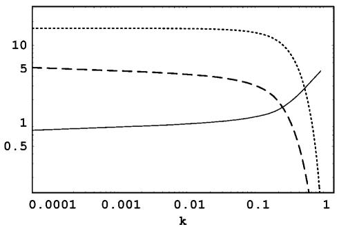
Figure 1: The dissipation constant $\kappa$ (dashed), the noise $\nu$ (dotted), both measured in units of $({\lambda}/{96\pi^{2}})^{2}$, and the effective temperature $T_{\rm eff}$ as functions of the scale $k$ for a fixed value of $T=0.5$.

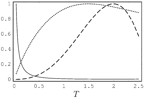
Figure 2: The dissipation constant $\kappa$ (dashed), the noise $\nu$ (dotted), both measured in units of $({\lambda}/{96\pi^{2}})^{2}$, and the effective temperature $T_{\rm eff}$ (solid), as functions of $T$ for a fixed value of $k=1/60$. Each quantity is normalized with respect to its maximum value in the displayed interval($\approx$ 215 for $\kappa$, 26 for $\nu$ and 10 for $T_{\rm eff}$).

The most important result of this paper is that RG running alone describes the onset of noise and dissipation in the long wavelength modes, even if these are not assumed to be present in the underlying microscopic theory. These two elements provide the sufficient conditions for thermalization as described by Schwinger [15, 16, 17, 18]. Therefore the model succeeds in describing the onset of the thermalization process, and yields simple estimates of both the final temperature and the thermalization times at different scales. We must caution however that in this form these estimates are not fully reliable, as they involve pushing the theory to the range $\Lambda T\geq 1$. This lies beyond the range of validity of our approximations concerning $T$. To extend the nonequilibrium RG to a larger $T$ range a fully self-consistent approach is necessary [28, 29, 30].

Because of this limitation, we do not claim to have solved the problem, but to have shown a framework for a solution. We need a self-consistent approach to the hard loops to be able to extend further the $T$ range. Still, the power of the nonequilibrium RG allows us to extend to the fully quantum regime the insights gained from wave turbulence in the classical stage of evolution.

References

References

- [1] Berges J 2004 Introduction to Nonequilibrium Quantum Field Theory Preprint hep-ph/0409233
- [2] Bassett B A, Tsujikawa S and Wands D 2006 Rev. Mod. Phys. 78 537
- [3] Felder G and Kofman L 2006 Nonlinear Inflaton Fragmentation after Preheating Preprint hep-ph/0606256.
- [4] Zakharov V E, L’vov V S and Falkovich G 1992 Kolmogorov spectra of turbulence I: wave turbulence (Berlin: Springer-Verlag)
- [5] Lombardo F and Mazzitelli F D 1996 Phys. Rev. D53 2001
- [6] Calzetta E, Hu B L and Mazzitelli F D 2001 Phys. Rep. 352 459
- [7] Polonyi J 2006 Phys. Rev. D 74 065014
- [8] Feynman R and Vernon F 1963 Ann. Phys. (NY) 24 118
- [9] Feynman R and Hibbs A 1965 Quantum Mechanics and Path Integrals (New York: McGraw - Hill)
- [10] Wilson K and Kogut J 1974 Phys. Rep. 12 75
- [11] Bodeker D 1998 Phys. Lett. B 426 351
- [12] Bodeker D 1999 Nuc. Phys. B 559 502
- [13] Litim D and Manuel C 2002 Phys. Rep. 364 451
- [14] Litim D 1998 Wilsonian flow equations and thermal field theory Preprint hep-ph/9811272
- [15] Schwinger J 1961 J. Math. Phys. 2 407
- [16] Keldysh L V 1964 Zh. Eksp. Teor. Fiz. 47 1515 [Engl. trans: Keldysh L V 1965 Sov. Phys. JEPT 20 1018 ]
- [17] Calzetta E and Hu B L 1987 Phys. Rev. D 35 495
- [18] Calzetta E and Hu B L 1988 Phys. Rev. D 37 2878
- [19] Dalvit D A R and Mazzitelli F D 1996 Phys. Rev. D 54 6338
- [20] Dalvit D A R 1998 Ph D Thesis (Universidad de Buenos Aires)
- [21] Zanella J and Calzetta E 2006 Renormalization group study of damping in nonequilibrium field theory Preprint hep-th/0611222
- [22] Peskin M E and Schroeder D V 1995 An Introduction to Quantum Field Theory (Perseus Books, Cambridge, Massachusetts)
- [23] Juchem S, Cassing W and Greiner C 2004 Phys. Rev. D 69 025006
- [24] Zanella J and Calzetta E 2006 Inflation and nonequilibrium renormalization group Preprint hep-ph/0611335
- [25] Callen H and Welton T 1951 Phys. Rev. 83 34
- [26] Landau L, Lifshitz E M and Pitaevsky L 1980 Statistical Physics vol 1 (London: Pergamon)
- [27] Lifshitz E M and Pitaievskii L P 1981 Physical Kinetics (Oxford: Pergamon Press)
- [28] Salmhofer M 2006 Dynamical Adjustment of Propagators in Renormalization Group Flows Preprint cond-mat/0607289
- [29] Litim D F and Pawlowsky J M 2006 Non-perturbative thermal flows and resummations Preprint hep-th/0609122
- [30] Blaizot J-P, Ipp A, Mendez-Galain R and Wschebor N 2006 Perturbation theory and non-perturbative renormalization flow in scalar field theory at finite temperature Preprint hep-ph/0610004