The $\gamma N\to\Delta$ transition in chiral effective-field theory

Abstract

We describe the pion electroproduction processes in the $\Delta$(1232)-resonance region within the framework of chiral effective-field theory. By studying the observables of pion electroproduction in a next-to-leading order calculation we are able to make predictions and draw conclusions on the properties of the $N\to\Delta$ electromagnetic form factors.

For the general overview and motivation of the electromagnetic $N\to\Delta$ transition we refer the reader to the opening part of these Proceedings and to our recent review Pascalutsa:2006up . In this short contribution we will focus on the chiral effective-field theoretic study of the $N\to\Delta$ transition.

1 Not-so-low energy expansion

The strength of chiral interactions goes with derivatives of pion fields which allows one to organize a perturbative expansion in powers of pion momentum and mass — the chiral perturbation theory ($\chi$PT) Weinberg:1978kz . The small expansion parameter is $p/{\Lambda}_{\chi SB}$, where $p$ is the momentum and ${\Lambda}_{\chi SB}\sim 4\pi f_{\pi}\approx 1$ GeV stands for the scale of spontaneous chiral symmetry breaking. Based on this expansion one should be able to systematically compute the pion-mass dependence of static quantities, such as nucleon mass, magnetic moments, as well as the momentum dependence of scattering processes, such as pion-pion and pion-nucleon scattering. This is an effective-field theory (EFT) expansion, in this case a low-energy expansion of QCD. One expects to obtain exactly the same answers as from QCD directly, provided the low-energy constants (LECs) — the parameters of the effective Lagrangian — are known, either from experiment or by matching to QCD itself (e.g., by fitting to the lattice QCD results).

One of the principal ingredients of an EFT expansion is power counting. The power counting assigns an order to Feynman graphs arising in loopwise expansion of the amplitudes, and thus defines which graphs need to be computed at a given order in the expansion. In a way it simply is a tool to estimate the size of different contributions without doing explicit calculations. The main requirement on a power-counting scheme is that it should estimate the relative size of various contributions correctly. In $\chi$PT with pions and nucleons alone GSS89 , the power counting for a graph with $L$ loops, $N_{\pi}$ ($N_{N}$) internal pion (nucleon) lines, and $V_{k}$ vertices from $k$th-order Lagrangian, estimates its contribution to go as $p^{n_{\chi\mathrm{PT}}}$, with the power given by:

$$n_{\chi\mathrm{PT}}=4L-2N_{\pi}-N_{N}+\sum_{k}kV_{k}\,.$$ (1)

Note that in the manifestly Lorentz-covariant formalism this power counting holds only in a specific renormalization scheme Gegelia:1999gf ; Pascalutsa:2005nd .

A cornerstone principle of effective field theories in general is naturalness, meaning that the dimensionless LECs must be of natural size, i.e., of order of unity. Any significant fine-tuning of even a single LEC leads, obviously, to a break-down of the EFT expansion. Therefore, even if an EFT describes the experimental data, but at the expense of fine-tuned LECs, the EFT expansion fails. Such an EFT can still be useful for getting insights into the physics beyond the EFT itself. Namely, by looking at the form of the fine-tuned operators, one might be able to deduce which contributions are missing.

For instance, it is known that the NLO $\chi$PT description of the pion-nucleon elastic scattering, near threshold, requires relatively large values for some of the LECs. It is not difficult to see that the operators corresponding with those unnatural LECs can be matched to the “integrated out” $\Delta$-resonance contributions. The problem is that the $\Delta$ is relatively light, its excitation energy, $\varDelta\equiv M_{\Delta}-M_{N}\sim 0.3$ GeV, is still quite small compared to ${\Lambda}_{\chi SB}\sim 1$ GeV. Integrating out the $\Delta$-isobar degrees of freedom corresponds to an expansion in powers of $p/\varDelta$, with $p\sim m_{\pi}$, which certainly is not as good of an expansion as the one in the meson sector, in powers of $p/{\Lambda}_{\chi SB}$.
The fine-tuning of the “Deltaless” $\chi$PT seems to be lifted by the inclusion of an explicit $\Delta$-isobar. Also, the limit of applicability of the EFT expansion is then extended to momenta of order of the resonance excitation energy, $p\sim\varDelta$. Such momenta can still be considered as soft, as long as $\varDelta/{\Lambda}_{\chi SB}$ can be treated as small. The resulting $\chi$PT with pion, nucleon, and $\Delta$-isobar degrees of freedom has two distinct light scales: $m_{\pi}$ and $\Delta$. Perhaps the most straightforward way to proceed is to organize a simultaneous expansion in two different small parameters:

$$\epsilon=m_{\pi}/{\Lambda}_{\chi SB}\,\,\,\,\mbox{and}\,\,\,\,\delta=\varDelta/{\Lambda}_{\chi SB}.$$

However, for power counting purposes it is certainly more convenient to have a single small parameter and thus a relation between $\epsilon$ and $\delta$ is usually imposed. We stress that the relation is established only at the level of power counting and not in the actual calculations of graphs. At present two such relations between $\epsilon$ and $\delta$ are used in the literature:

• $\epsilon\sim\delta$, the so-called “Small Scale Expansion” JeM91a ; HHK97 , here refered to as the “$\epsilon$-expansion”;
  

• $\epsilon\sim\delta^{2}$, the “$\delta$-expansion” Pascalutsa:2002pi .

The table below (Table 1) summarizes the counting of momenta in the three expansions: Deltaless ($\Delta\!\!\!\!/$-$\chi$PT), $\epsilon$-expansion, and $\delta$-expansion.

EFT	$\quad p\sim m_{\pi}\quad$	$\quad p\sim\Delta\quad$
$\Delta\!\!\!\!/$-$\chi$PT	${\mathcal{O}}(p)$	${\mathcal{O}}(1)$
$\epsilon$-expansion	${\mathcal{O}}(\epsilon)$	${\mathcal{O}}(\epsilon)$
$\delta$-expansion	${\mathcal{O}}(\delta^{2})$	${\mathcal{O}}(\delta)$

Table 1: The counting of momenta in the three different $\chi$EFT expansions.

An unsatisfactory feature of the $\epsilon$-expansion is that the $\Delta$-resonance contributions are always estimated to be of the same size as the nucleon contributions. In reality (revealed by actually computing these contributions), they are suppressed at low energies and dominate in the the $\Delta$-resonance region. Thus, apparently the power-counting in the $\epsilon$-expansion overestimates the $\Delta$-contributions at lower energies and underestimates them at the resonance energies. The $\delta$-expansion improves on this aspect, as is briefly described in what follows.
In the $\delta$-expansion, the power counting depends on the energy domain, since in the low-energy region ($p\sim m_{\pi}$) and the resonance region ($p\sim\varDelta$), the momentum counts differently, see Table 1. This dependence most significantly affects the power counting of the direct resonance exchanges — the one-Delta-reducible (ODR) graphs. Figure 1 illustrates examples of the ODR graphs for the case of Compton scattering on the nucleon. These graphs are all characterized by having a number of ODR propagators, each going as

$$S_{ODR}\sim\frac{1}{s-M_{\Delta}^{2}}\sim\frac{1}{2M_{\Delta}}\frac{1}{p-\varDelta}\,,$$ (2)

where $p$ is the soft momentum, in this case given by the photon energy. In contrast the nucleon propagator in analogous graphs would go simply as $S_{N}\sim 1/p$.

Figure 1: Examples of the one-Delta-reducible (1st row) and the one-Delta-irreducible (2nd row) graphs in Compton scattering.

Therefore, in the low-energy region, the $\Delta$ and nucleon propagators would count respectively as ${\mathcal{O}}(1/\delta)$ and ${\mathcal{O}}(1/\delta^{2})$, the $\Delta$ being suppressed by one power of the small parameter as compared to the nucleon. In the resonance region, the ODR graphs obviously all become large. Fortunately they all can be subsumed, leading to “dressed” ODR graphs with a definite power-counting index. Namely, it is not difficult to see that the resummation of the classes of ODR graphs results in ODR graphs with only a single ODR propagator of the form

$$S_{ODR}^{\ast}=\frac{1}{S_{ODR}^{-1}-\Sigma}\sim\frac{1}{p-\varDelta-\Sigma}\,,$$ (3)

where $\Sigma$ is the $\Delta$ self-energy. The expansion of the self-energy begins with $p^{3}$, and hence in the low-energy region does not affect the counting of the $\Delta$ contributions. However, in the resonance region the self-energy not only ameliorates the divergence of the ODR propagator at $s=M_{\Delta}^{2}$ but also determines power-counting index of the propagator. Defining the $\Delta$-resonance region formally as the region of $p$ where

$$|p-\varDelta|\leq\delta^{3}{\Lambda}_{\chi SB}\,,$$ (4)

we deduce that an ODR propagator, in this region, counts as ${\mathcal{O}}(1/\delta^{3})$. Note that the nucleon propagator in this region counts as ${\mathcal{O}}(1/\delta)$, hence is suppressed by two powers as compared to ODR propagators. Thus, within the power-counting scheme we have the mechanism for estimating correctly the relative size of the nucleon and $\Delta$ contributions in the two energy domains. In Table 2 we summarize the counting of the nucleon, ODR, and one-Delta-irreducible (ODI) propagators in both the $\epsilon$- and $\delta$-expansion.

	$\epsilon$-expansion	$\delta$-expansion
	$p/{\Lambda}_{\chi SB}\sim\epsilon$	$p\sim m_{\pi}$	$p\sim\varDelta$
$\,S_{N}\,$	$1/\epsilon$	$1/\delta^{2}$	$1/\delta$
$\,S_{ODR}\,$	$1/\epsilon$	$1/\delta$	$1/\delta^{3}$
$\,S_{ODI}\,$	$1/\epsilon$	$1/\delta$	$1/\delta$

Table 2: The counting for the nucleon, one-Delta-reducible (ODR), and one-Delta-irreducible (ODI) propagators in the two different expansion schemes. The counting in the $\delta$-expansion depends on the energy domain.

We conclude this discussion by giving the general formula for the power-counting index in the $\delta$-expansion. The power-counting index, $n$, of a given graph simply tells us that the graph is of the size of ${\mathcal{O}}(\delta^{n})$. For a graph with $L$ loops, $V_{k}$ vertices of dimension $k$, $N_{\pi}$ pion propagators, $N_{N}$ nucleon propagators, $N_{\Delta}$ Delta propagators, $N_{ODR}$ ODR propagators and $N_{ODI}$ ODI propagators (such that $N_{\Delta}=N_{ODR}+N_{ODI}$) the index is

$$n=\left\{\begin{array}[]{cc}2n_{\chi\mathrm{PT}}-N_{\Delta}\,,&p\sim m_{\pi};\\ n_{\chi\mathrm{PT}}-3N_{ODR}-N_{ODI}\,,&p\sim\Delta,\end{array}\right.$$

where $n_{\chi\mathrm{PT}}$, given by Eq. (1), is the index of the graph in $\chi$PT with no $\Delta$’s. For further details on the $\delta$ counting we refer to Ref. Pascalutsa:2002pi .

The $\gamma N\Delta$ form factors have been examined in both the $\epsilon$-expansion Gellas:1998wx ; Gail and the $\delta$-expansion Pascalutsa:2005ts ; Pascalutsa:2005vq . In the following we focus on the latter analysis.

2 Pion electroproduction to next-to-leading order

The $N\to\Delta$ transition can be induced by a pion or a photon. The correponding effective Lagrangians are written as:

$${\mathcal{L}}^{(1)}_{N\Delta} = \frac{ih_{A}}{2f_{\pi}M_{\Delta}}\overline{N}\,T^{a}\,\gamma^{\mu\nu\lambda}\,(\partial_{\mu}\Delta_{\nu})\,\partial_{\lambda}\pi^{a}+\mbox{H.c.},$$ (5a)

$${\mathcal{L}}^{(2)}_{N\Delta} = \frac{3ieg_{M}}{2M_{N}(M_{N}+M_{\Delta})}\,\overline{N}\,T^{3}\,(\partial_{\mu}\Delta_{\nu})\,\tilde{F}^{\mu\nu}+\mbox{H.c.},$$ (5b)

$${\mathcal{L}}^{(3)}_{N\Delta} = \frac{-3e}{2M_{N}(M_{N}+M_{\Delta})}\overline{N}\,T^{3}\gamma_{5}\left[g_{E}(\partial_{\mu}\Delta_{\nu})+\frac{ig_{C}}{M_{\Delta}}\gamma^{\alpha}(\partial_{\alpha}\Delta_{\nu}-\partial_{\nu}\Delta_{\alpha})\,\partial_{\mu}\right]F^{\mu\nu}+\mbox{H.c.},\;\;\;\;\;$$ (5c)

where $N$, $\Delta_{\mu}$, $\pi$ stand respectively for the nucleon (spinor, isodublet), $\Delta$-isobar (vector-spinor, isoquartet), pion (pseudoscalar, isovector) fields; $F^{\mu\nu}$ and $\tilde{F}^{\mu\nu}$ are the electromagnetic field strength and its dual, $T^{a}$ are the isospin-1/2-to-3/2 transition $(2\times 4$) matrices. The coupling constants $h_{A}$, $g_{M}$, $g_{E}$, and $g_{C}$ are the LECs describing the $N\to\Delta$ tansition at the tree level.

The $\gamma N\to\Delta$ transition is traditionally studied in the process of pion electroproduction on the nucleon. Let us consider this process to NLO in the $\delta$ expansion. Since we are using the one-photon-exchange approximation, the pion photoproduction can be viewed as the particular case of electroproduction at $Q^{2}=0$.

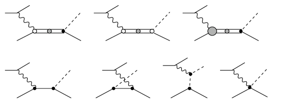
Figure 2: Diagrams for the $eN\to e\pi N$ reaction to LO and NLO in the $\delta$-expansion. The dots denote the vertices from the 1st-order Lagrangian, while the circles are the vertices from the 2nd order Lagrangian (e.g., the $\gamma N\Delta$-vertex in the first two graphs is the $g_{M}$ coupling from ${\mathcal{L}}^{(2)}$).

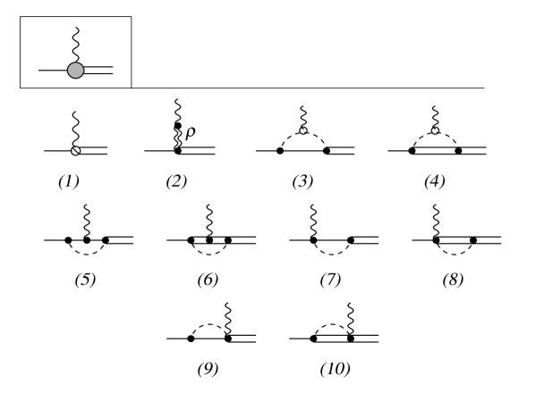
Figure 3: The $\gamma N\Delta$ vertex at ${\mathcal{O}}(\delta^{3})$. The sliced vertex (1) stands for the $g_{E}$ and $g_{C}$ couplings from the 3rd order Lagrangian. The wiggly double line in (2) stands for the vector-meson propagator.

The pion electroproduction amplitude to NLO in the $\delta$-expansion, in the resonance region, is given by the graphs in Fig. 2, where the shaded blob in the 3rd graph denotes the NLO $\gamma N\Delta$ vertex, given by the graphs in Fig. 3. The 1st graph in Fig. 2 enters at the LO, which here is ${\mathcal{O}}(\delta^{-1})$. All the other graphs in Fig. 2 are of NLO$={\mathcal{O}}(\delta^{0})$. Note that the $\Delta$-resonance contribution at NLO is obtained by going to NLO in either the $\pi N\Delta$ vertex (2nd graph) or the $\gamma N\Delta$ vertex (3rd graph). Accordingly, the $\Delta$ self-energy in these graphs is included, respectively, to NLO. The vector-meson diagram, Fig. 3(2), contributes to NLO for $Q^{2}\sim{\Lambda}\Delta$. One includes it effectively by giving the $g_{M}$-term a dipole $Q^{2}$-dependence (in analogy to how it is usually done for the nucleon isovector form factor):

$$g_{M}\to\frac{g_{M}}{(1+Q^{2}/0.71\,\mbox{GeV}^{2})^{2}}.$$ (6)

The analogous effect for the $g_{E}$ and $g_{C}$ couplings begins at N²LO.
An important observation is that at $Q^{2}=0$ only the imaginary part (unitarity cut) of the loop graphs in Fig. 3 contributes to the NLO amplitude. Their real-part contributions, after the renormalization of the LECs, begin to contribute at N²LO, for $Q^{2}\ll\varDelta{\Lambda}_{\chi SB}$. At present we will consider only the NLO calculation where the $\pi\Delta$-loop contributions to the $\gamma N\Delta$-vertex are omitted since they do not give the imaginary contributions in the $\Delta$-resonance region. We emphasize that such loops might become important at this order for $Q^{2}\sim\varDelta{\Lambda}_{\chi SB}\sim 0.3$ GeV² and should be included for the complete NLO result. The present calculation is thus restricted to values $Q^{2}<0.3$ GeV².

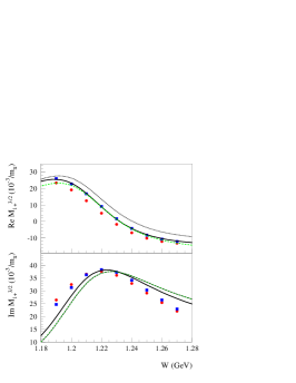
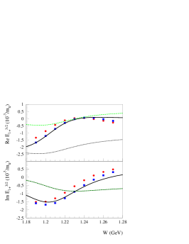
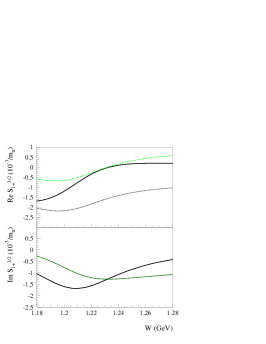
Figure 4: (Color online) The $M_{1+}^{(3/2)}$, $E_{1+}^{(3/2)}$, and $S_{1+}^{(3/2)}$ multipoles for pion photoproduction as function of the invariant energy. Green dashed curves: $\Delta$ contribution without the $\gamma N\Delta$-vertex loop corrections, [i.e., only the first three graphs in Fig. 2 with Fig. 3(1) contribution are taken into account]. Blue dotted curves: adding the Born contributions, 2nd line in Fig. 2, to the dashed curves. Black solid curves: the NLO calculation, includes all graphs in Fig. 2 as well as the loop corrections. The data point are from the SAID analysis (FA04K) GWU (red circles), and from the MAID 2003 analysis MAID (blue squares).

In Fig. 4 shown are the resonant multipoles $M_{1+}^{(3/2)}$, $E_{1+}^{(3/2)}$, and $S_{1+}^{(3/2)}$ as function of the invariant energy $W=\sqrt{s}$ around the resonance position and $Q^{2}=0$. The $M_{1+}^{(3/2)}$ and $E_{1+}^{(3/2)}$ multipoles are well established by the SAID GWU and MAID MAID empirical partial-wave solutions, thus allowing one to fit two of the three $\gamma N\Delta$ LECs at this order as: $g_{M}=2.97$, $g_{E}=-1.0$. The third LEC is adjusted to for a best description of the pion electroproduction data at low $Q^{2}$ (see ), yielding $g_{C}=-2.6$. The latter values translate into $G_{M}^{\ast}=3.04$, $G_{E}^{\ast}=0.07$, and $G_{C}^{\ast}=1.00$ for the Jones–Scadron form-factors Jones:1972ky at $Q^{2}=0$. As is seen from the figure, the NLO results (solid curves) give a good description of the energy dependence of the resonant multipoles in a window of 100 MeV around the $\Delta$-resonance position. These values yield $R_{EM}=-2.2$ % and $R_{SM}=-3.4$ %.

The dashed curves in these figures show the contribution of the $\Delta$-resonant diagram of Fig. 2 without the NLO loop corrections in Fig. 3. For the $M_{1+}$ multipole this is the LO and part of the NLO contributions. For the $E_{1+}$ and $S_{1+}$ multipole the LO contribution is absent (recall that $g_{E}$ and $g_{C}$ coupling are of one order higher than the $g_{M}$ coupling). Hence, the dashed curve represents a partial NLO contribution to $E_{1+}$ and $S_{1+}$.

Note that such a purely resonant contribution without the loop corrections satisfies unitarity in the sense of the Fermi-Watson theorem, which states that the phase of a pion electroproduction amplitude ${\mathcal{M}}_{l}$ is given by the corresponding pion-nucleon phase-shift: ${\mathcal{M}}_{l}=|{\mathcal{M}}_{l}|\,\exp({i\delta_{l}})$. As a direct consequence of this theorem, the real-part of the resonant multipoles must vanish at the resonance position, where the phase-shift crosses $90$ degrees.

Upon adding the non-resonant Born graphs (2nd line in Fig. 2) to the dashed curves, one obtains the dotted curves. The non-resonant contributions are purely real at this order and hence the imaginary part of the multipoles do not change. While this is consistent with unitarity for the non-resonant multipoles (recall that the non-resonant phase-shifts are zero at NLO), the Fermi-Watson theorem in the resonant channels is violated. In particular, one sees that the real parts of the resonant multipoles now fail to cross zero at the resonance position. The complete NLO calculation, shown by the solid curves in the figure includes in addition the $\pi N$-loop corrections in Fig. 3, which restore unitarity. The Fermi-Watson theorem is satisfied exactly in this calculation.

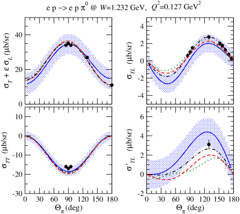
Figure 5: The pion angular dependence of the $\gamma^{\ast}p\to\pi^{0}p$ cross sections at $W=1.232$ GeV and $Q^{2}$ = 0.127 GeV². Dashed-dotted (black) curves: DMT model KY99 . Dashed (red) curves: SL model SL . Dotted (green) curves : DUO model DUO . Solid (blue) curves: $\chi$EFT results Pascalutsa:2005ts ; Pascalutsa:2005vq . The bands provide an estimate of the theoretical error for the $\chi$EFT calculations. Data points are from BATES experiments Mertz:1999hp ; Kunz:2003we ; Sparveris:2004jn .

In Fig. 5, the different virtual photon absorption cross sections around the resonance position are displayed at $Q^{2}=0.127$ GeV², where recent precision data are available. We compare these data with the present $\chi$EFT calculations as well as with the results of SL, DMT, and DUO models SL ; KY99 ; DUO .

In the $\chi$EFT calculations, the low-energy constants $g_{M}$ and $g_{E}$, were fixed from the resonant pion photoproduction multipoles. Therefore, the only other low-energy constant from the chiral Lagrangian entering the NLO calculation is $g_{C}$. The main sensitivity on $g_{C}$ enters in $\sigma_{TL}$. A best description of the $\sigma_{TL}$ data at low $Q^{2}$ is obtained by choosing $g_{C}=-2.6$.

From the figure one sees that the NLO $\chi$EFT calculation, within its accuracy, is consistent with the experimental data for these observables at low $Q^{2}$. The dynamical models are in basic agreement with each other and the data for the transverse cross sections. Differences between the models do show up in the $\sigma_{TL}$ and $\sigma_{TL^{\prime}}$ cross sections which involve the longitudinal amplitude. In particular for $\sigma_{TL^{\prime}}$ the differences reflect to a large extent how the non-resonant $S_{0+}$ multipole is described in the models.

3 Pion-mass dependence of the $\gamma N\Delta$ form factors

Since the low-energy constants $g_{M}$, $g_{E}$, and $g_{C}$ have been fixed, our calculation can provide a prediction for the $m_{\pi}$ dependence of the $\gamma N\Delta$ transition form factors. The study of the $m_{\pi}$-dependence is crucial to connect to lattice QCD results, which at present can only be obtained for larger pion masses (typically $m_{\pi}\gtrsim 300$ MeV).

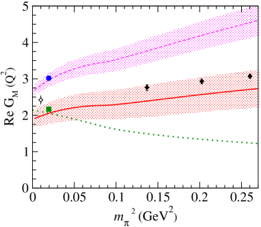
Figure 6: The pion mass dependence of the real part of the Jones-Scadron $\gamma^{*}N\Delta$ form factor $G_{M}^{\ast}$ for $Q^{2}=0$ and $Q^{2}$ = 0.127 GeV² in the $\chi$EFT framework. The solid (dashed) curves are the NLO results for $Q^{2}=0.127$ GeV² ($Q^{2}=0$) respectively, including the $m_{\pi}$ dependence of $M_{N}$ and $M_{\Delta}$. The green dotted curve is the corresponding result for $Q^{2}=0.127$ GeV² where the $m_{\pi}$ dependence of $M_{N}$ and $M_{\Delta}$ is not included. The blue circle for $Q^{2}=0$ is a data point from MAMI Beck:1999ge , and the green square for $Q^{2}=0.127$ GeV² is a data point from BATES Mertz:1999hp ; Sparveris:2004jn . The three filled black diamonds at larger $m_{\pi}$ are lattice calculations Alexandrou:2004xn for $Q^{2}$ values of 0.125, 0.137, and 0.144 GeV² respectively, whereas the open diamond near $m_{\pi}\simeq 0$ represents their extrapolation assuming linear dependence in $m_{\pi}^{2}$.

In Fig. 6 we examine the $m_{\pi}$-dependence of the magnetic $\gamma N\Delta$-transition form factor $G_{M}^{\ast}$, in the convention of Jones and Scadron Jones:1972ky . At the physical pion mass, this form factor can be obtained from the imaginary part of the $M_{1+}^{3/2}$ multipole at $W=M_{\Delta}$ (where the real part is zero by Watson’s theorem). The value of $G_{M}^{\ast}$ at $Q^{2}=0$ is determined by the low-energy constant $g_{M}$. The $Q^{2}$-dependence then follows as a prediction of the NLO result, and Fig. 6 shows that this prediction is consistent with the experimental value at $Q^{2}=0.127$ GeV² and physical pion mass.

The $m_{\pi}$-dependence of $G_{M}^{\ast}$ is also completely fixed at NLO, no new parameters appear. In Fig. 6, the result for $G_{M}^{\ast}$ at $Q^{2}=0.127$ GeV² is shown both when the $m_{\pi}$-dependence of the nucleon and $\Delta$ masses is included (solid line) and when it is not (dotted line). Accounting for the $m_{\pi}$-dependence in $M_{N}$ and $M_{\Delta}$, significantly affects $G_{M}^{\ast}$. The $\chi$EFT  calculation, with the $m_{\pi}$ dependence of $M_{N}$ and $M_{\Delta}$ included, is in a qualitatively good agreement with the lattice data shown in the figure. The $\chi$EFT result also follows an approximately linear behavior in $m_{\pi}^{2}$, although it falls about 10 - 15 % below the lattice data. This is just within the uncertainty of the NLO results. One should also keep in mind that the present lattice simulations are not done in full QCD, but are “quenched”, so discrepancies are not unexpected.

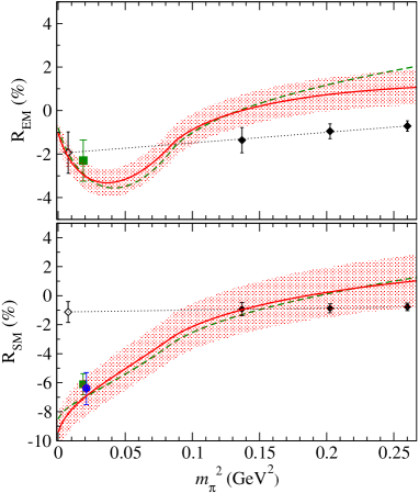
Figure 7: The pion mass dependence of $R_{EM}$ (upper panel) and $R_{SM}$ (lower panel), at $Q^{2}=0.1$ GeV². The blue circle is a data point from MAMI Pospischil:2000ad , the green squares are data points from BATES Mertz:1999hp ; Sparveris:2004jn . The three filled black diamonds at larger $m_{\pi}$ are lattice calculations Alexandrou:2004xn , whereas the open diamond near $m_{\pi}\simeq 0$ represents their extrapolation assuming linear dependence in $m_{\pi}^{2}$. Red solid curves: NLO result when accounting for the $m_{\pi}$ dependence in $M_{N}$ and $M_{\Delta}$; green dashed curves: NLO result of Ref. Pascalutsa:2005ts , where the $m_{\pi}$-dependence of $M_{N}$ and $M_{\Delta}$ was not accounted for. The error bands represent the estimate of theoretical uncertainty for the NLO calculation.

In Fig. 7, we show the $m_{\pi}$-dependence of the ratios $R_{EM}$ and $R_{SM}$ and compare them to lattice QCD calculations. The recent state-of-the-art lattice calculations of $R_{EM}$ and $R_{SM}$ Alexandrou:2004xn use a linear, in the quark mass ($m_{q}\propto m_{\pi}^{2}$), extrapolation to the physical point, thus assuming that the non-analytic $m_{q}$-dependencies are negligible. The thus obtained value for $R_{SM}$ at the physical $m_{\pi}$ value displays a large discrepancy with the experimental result, as seen in Fig. 7. Our calculation, on the other hand, shows that the non-analytic dependencies are not negligible. While at larger values of $m_{\pi}$, where the $\Delta$ is stable, the ratios display a smooth $m_{\pi}$ dependence, at $m_{\pi}=\Delta$ there is an inflection point, and for $m_{\pi}\leq\Delta$ the non-analytic effects are crucial, as was also observed for the $\Delta$-resonance magnetic moment Cloet03 ; PV05 .

One also sees from Fig. 7 that, unlike the result for $G_{M}^{\ast}$, there is little difference between the $\chi$EFT calculations with the $m_{\pi}$-dependence of $M_{N}$ and $M_{\Delta}$ accounted for, and our earlier calculation Pascalutsa:2005ts , where the ratios were evaluated neglecting the $m_{\pi}$-dependence of the masses. This is easily understood, as the main effect due to the $m_{\pi}$-dependence of $M_{N}$ and $M_{\Delta}$ arises due to a common factor in the evaluation of the $\gamma N\Delta$ form factors, which drops out of the ratios. One can speculate that the “quenching” effects drop out, at least partially, from the ratios as well. In Fig. 7 we also show the $m_{\pi}$-dependence of the $\gamma N\Delta$ transition ratios, with the theoretical error band. The $m_{\pi}$ dependence obtained here from $\chi$EFT  clearly shows that the lattice results for $R_{SM}$ may in fact be consistent with experiment.

4 Conclusion

We presented here an extension of the chiral perturbation theory framework to the energy domain of $\Delta$(1232). In this extension the $\Delta$-isobar appears as an explicit degree of freedom in the effective chiral Lagrangian. The other low-energy degrees of freedom appearing in this Lagrangian are pions, nucleons, and $\rho$-mesons. The power counting depends crucially on how the $\Delta$-resonance excitation energy, $\varDelta=M_{\Delta}-M_{N}$, compares to the other scales in the problem. In the “$\delta$-expansion” scheme adopted here, one utilizes the scale hierarchy, $m_{\pi}\ll\varDelta\ll{\Lambda}_{\chi SB}$. In other words, we have an EFT with two distinct light scales. Such a scale hierarchy is crucial for an adequate counting of the $\Delta$-resonance contributions in both the low-energy and the resonance energy regions. The $\delta$ power counting provides a justification for “integrating out” the resonance contribution at very low energies, as well as for resummation of certain resonant contributions in the resonance region.

We applied the $\delta$-expansion to the process of pion electroproduction. This is a first $\chi$EFT study of this reaction in the $\Delta(1232)$-resonance region. Our resulting next-to-leading order calculation was shown to satisfy the electromagnetic gauge and chiral symmetries, Lorentz-covariance, analyticity, unitarity (Watson’s theorem). The free parameters entering at this order are the $\gamma N\Delta$ couplings $g_{M}$, $g_{E}$, $g_{C}$ characterizing the $M1$, $E2$, $C2$ transitions, respectively. By comparing our NLO results with the standard multipole solutions (MAID and SAID) for the photoproduction multipoles we have extracted $g_{M}$ = 2.97 and $g_{E}=-1.0$, corresponding to $R_{EM}=-2.2$ %. The NLO $\chi$EFT result was also found to give a good description of the energy-dependence of most non-resonant $s$, $p$ and $d$-wave photoproduction multipoles in a 100 MeV window around the $\Delta$-resonance position. From the pion electroproduction cross-section $\sigma_{LT}$ we have extracted $g_{C}=-2.6$, which yields $R_{SM}\simeq-7$ % near $Q^{2}=0.127$ GeV². In overall, the NLO results are consistent with the experimental data of the recent high-precision measurements at MAMI and BATES.

The $\chi$EFT framework plays a dual role in that it allows for an extraction of resonance parameters from observables and predicts their pion-mass dependence. In this way it may provide a crucial connection of present lattice QCD results (obtained at larger than physical values of $m_{\pi}$) to the experiment. We have shown here that the opening of the $\Delta\to\pi N$ decay channel at $m_{\pi}=M_{\Delta}-M_{N}$ induces a pronounced non-analytic behavior of the $R_{EM}$ and $R_{SM}$ ratios. While the linearly-extrapolated lattice QCD results for $R_{SM}$ are in disagreement with experimental data, the $\chi$EFT prediction of the non-analytic dependencies suggests that these results are in fact consistent with experiment.

The presented results are systematically improvable. We have indicated what are the next-next-to-leading order effects, however, at present we could only estimate the theoretical uncertainty of our calculations due to such effects. We have defined and provided a corresponding error band on our NLO results. An actual calculation of N²LO effects is a worthwhile topic for a future work.

References

- (1) V. Pascalutsa, M. Vanderhaeghen and S. N. Yang, Phys. Rep. (in press) [arXiv:hep-ph/0609004].
- (2) S. Weinberg, Physica A 96, 327 (1979); J. Gasser and H. Leutwyler, Annals Phys. 158, 142 (1984).
- (3) J. Gasser, M. E. Sainio and A. Svarc, Nucl. Phys. B 307, 779 (1988).
- (4) J. Gegelia and G. Japaridze, Phys. Rev. D 60, 114038 (1999); J. Gegelia, G. Japaridze and X. Q. Wang, J. Phys. G 29, 2303 (2003).
- (5) V. Pascalutsa and M. Vanderhaeghen, Phys. Lett. B 636, 31 (2006).
- (6) E. Jenkins and A. V. Manohar, Phys. Lett. B 255, 558 (1991).
- (7) T. Hemmert, B. R. Holstein and J. Kambor, Phys. Lett. B 395, 89 (1997); J. Phys. G 24, 1831 (1998).
- (8) V. Pascalutsa and D. R. Phillips, Phys. Rev. C 67, 055202 (2003); ibid. 68, 055205 (2003).
- (9) G. C. Gellas, T. R. Hemmert, C. N. Ktorides and G. I. Poulis, Phys. Rev. D 60, 054022 (1999).
- (10) T. A. Gail and T. R. Hemmert, arXiv:nucl-th/0512082; see also the contribution of T. Gail to these proceedings.
- (11) V. Pascalutsa and M. Vanderhaeghen, Phys. Rev. Lett. 95, 232001 (2005).
- (12) V. Pascalutsa and M. Vanderhaeghen, Phys. Rev. D 73, 034003 (2006).
- (13) V. Pascalutsa, C. E. Carlson and M. Vanderhaeghen, Phys. Rev. Lett. 96, 012301 (2006).
- (14) S. Kondratyuk and P. G. Blunden, Nucl. Phys. A 778, 44 (2006) [arXiv:nucl-th/0601063].
- (15) R. A. Arndt, W. J. Briscoe, I. I. Strakovsky and R. L. Workman, Phys. Rev. C 66, 055213 (2002) [SAID website, http://gwdac.phys.gwu.edu].
- (16) D. Drechsel, O. Hanstein, S. S. Kamalov and L. Tiator, Nucl. Phys. A 645, 145 (1999) [MAID website, http://www.kph.uni-mainz.de].
- (17) H. F. Jones and M. D. Scadron, Ann. Phys. 81, 1 (1973).
- (18) T. Sato and T.-S.H. Lee, Phys. Rev. C 54, 2660 (1996); ibid. 63, 055201 (2001).
- (19) S. S. Kamalov and S. N. Yang, Phys. Rev. Lett. 83, 4494 (1999); S. S. Kamalov, S. N. Yang, D. Drechsel, O. Hanstein, and L. Tiator, Phys. Rev. C 64, 032201(R) (2001).
- (20) V. Pascalutsa and J. A. Tjon, Phys. Rev. C 61, 054003 (2000); ibid. 70, 035209 (2004); G. L. Caia et al., Phys. Rev. C 70, 032201(R) (2004); ibid. 72, 035203 (2005).
- (21) C. Mertz et al., Phys. Rev. Lett. 86, 2963 (2001).
- (22) C. Kunz et al., Phys. Lett. B 564, 21 (2003).
- (23) N. F. Sparveris et al. [OOPS Collaboration], Phys. Rev. Lett. 94, 022003 (2005); see also the contribution of Nikos Sparveris to these proceedings.
- (24) R. Beck et al., Phys. Rev. C 61, 035204 (2000).
- (25) C. Alexandrou, P. de Forcrand, H. Neff, J. W. Negele, W. Schroers and A. Tsapalis, Phys. Rev. Lett. 94, 021601 (2005); see also the contribution of C. Alexandrou to these proceedings.
- (26) T. Pospischil et al., Phys. Rev. Lett. 86, 2959 (2001).
- (27) I. C. Cloet, D. B. Leinweber and A. W. Thomas, Phys. Lett. B 563, 157 (2003); R. D. Young, D. B. Leinweber and A. W. Thomas, Nucl. Phys. Proc. Suppl. 129, 290 (2004).
- (28) V. Pascalutsa and M. Vanderhaeghen, Phys. Rev. Lett. 94, 102003 (2005).