Fermion resonance in quantum field theory

Abstract

We derive accurately the fermion resonance propagator by means of Dyson summation of the self-energy contribution. It turns out that the relativistic fermion resonance differs essentially from its boson analog.

I Introduction

The Breit-Wigner formula describing the processes of production and decay of unstable particle is widely used in hadron and nuclear physics. The original formula BW , which was applied to scattering of slow neutrons, is a non-relativistic one with energy-independent parameters – resonance position and width. It is clear that the simplest Breit-Wigner formula is applicable only for narrow states and description of a resonance curve for broad hadron resonances (at high experimental accuracy) needs some improved resonance formula. In hadron phenomenology there exist slightly different methods to describe resonance contribution but practically all methods are based on (effective) quantum field theory.

In spite of long history we found with some astonishment that situation with description of fermion resonance is not so evident up to now. Naively one can expect that the fermion resonance contribution to cross-section is the same as the boson one. Such point of view may be found in many papers and reviews, in particular, in Yao .But this is not the case, as it is seen from our consideration. First of all, the natural variable in fermion case is $W=\sqrt{s}$ but not $s$, so the fermion resonance factor will be $W$-dependent. After renormalization of dressed propagator one can see that the fermion specifics is generated by antisymmetric in $W$ contributions in a self-energy. This property is easily seen with use of the off-shell projection operators instead of $\gamma$-matrices.

Below we derive the Breit-Wigner-like formula for fermions in quantum field theory and discuss some its properties. We found that the so obtained dressed propagator (20) has some interesting features specific for fermions.

II Boson resonance in QFT

Let us first consider a more evident case of the boson resonance. The unstable particle is usually associated with the Breit-Wigner formula for an amplitude

$$T(a\to R\to b)=g_{a}\cdot\dfrac{1}{M_{R}^{2}-s-i\Gamma_{R}M_{R}}\cdot g_{b}.$$ (1)

Here the factor $G(s)=1/(M_{R}^{2}-s-i\Gamma_{R}M_{R})$ represents relativistic propagator of unstable particle.

The similar formula may be obtained in framework of quantum field theory by means of Dyson summation of the self-energy insertions into propagator. Equivalently, we should solve the Dyson-Schwinger equation for dressed nonrenormalized propagator

$$G=G_{0}+GJG_{0}.$$ (2)

Here $G_{0}(s)=(M^{2}-s)^{-1}$ and $G(s)$ are the bare and total propagators respectively, $J(s)$ is the self-energy contribution (sum of the 1PI diagrams).

The equation (2) may be rewritten in terms of inverse propagators $S(s)=G^{-1}(s)$

$$S=S_{0}-J=M^{2}-s-J(s).$$ (3)

If to use the on-mass-shell scheme of renormalization, then $M$ is the renormalized mass and one should subtract the self-energy contribution twice at this point

$$S^{r}=M^{2}-s-[J(s)-\mathrm{Re}\,J(M^{2})-\mathrm{Re}\,J^{\prime}(M^{2})(s-M^{2})].$$ (4)

After it we have formula similar to (1) but with ”running” mass and width. From QFT point of view the Breit-Wigner formula is rather rough approach, when we neglect by the energy dependence in mass and width (i.e. by the energy dependence in loop contribution $J(s)$). Such simplification is justified only for narrow resonance located far from threshold.

III Fermion resonance in QFT

III.1 Dressing and renormalization

Dressing of the fermion propagator looks rather similar:

$$G_{0}(p)=\frac{1}{\hat{p}-M}\ \ \Rightarrow\ \ G(p)=\frac{1}{\hat{p}-M-\Sigma(p)},$$ (5)

where $\Sigma(p)=A(p^{2})+\hat{p}B(p^{2})$ is a self-energy contribution.

To renormalize the obtained expression it is convenient to work with the inverse propagator $S(p)=G^{-1}(p)$. Usually the renormalization condition is formulated as the decomposition of inverse propagator in terms of $\hat{p}-M$

$$S(p)=\hat{p}-M+o(\hat{p}-M)\quad\text{at}\quad\hat{p}\to M.$$ (6)

Useful technical step is to introduce the basis of the off-shell projection operators $\Lambda^{\pm}$

$$\Lambda^{\pm}=\dfrac{1}{2}\big{(}1\pm\frac{\hat{p}}{W}\big{)},\quad W=\sqrt{p^{2}},$$ (7)

which simplifies all operations with $\gamma$-matrices and makes more clear the renormalization procedure. For illustration, let us use this basis for the self-energy contribution. Evident chain gives:

$$\Sigma(p) = A(p^{2})+\hat{p}B(p^{2})=(\Lambda^{+}+\Lambda^{-})A(W^{2})+W(\Lambda^{+}-\Lambda^{-})B(W^{2})$$ (8)

$$= \Lambda^{+}[A(W^{2})+WB(W^{2})]+\Lambda^{-}[A(W^{2})-WB(W^{2})].$$

One can see that coefficients $\Sigma^{\pm}$ in this basis are related by simple substitution $\Sigma^{-}(W)=\Sigma^{+}(-W)$ and dressed propagator has this property also.

The reversing of propagator is very easy due to simple multiplicative properties of the basis. If the inverse propagator has a decomposition

$$S(p)=\Lambda^{+}S^{+}(W)+\Lambda^{-}S^{-}(W),$$ (9)

with the symmetry property $S^{-}(W)=S^{+}(-W)$, then the propagator $G(p)$ is of the form

$$G(p)=\Lambda^{+}\frac{1}{S^{+}(W)}+\Lambda^{-}\frac{1}{S^{-}(W)}.$$ (10)

So, the explicit form of dressed unrenormalized propagator is evident:

$$G(p)=\Lambda^{+}\dfrac{1}{W-M-(A(W^{2})+WB(W^{2}))}+\Lambda^{-}\dfrac{1}{-W-M-(A(W^{2})-WB(W^{2}))}.$$ (11)

Thus, using the $\Lambda$-basis we have separated the $\gamma$-matrix structure and should renormalize the scalar coefficients dependent on $W$. More exactly, we need renormalize only $G^{+}(W)$ component, after that another coefficient $G^{-}(W)$ is obtained by substitution $W\to-W$.

For bound state, located below the threshold, the renormalization leads to the following condition for the self-energy contribution:

$$S^{+}=W-M+o(W-M)\quad\text{at}\quad W\to M.$$

One can convince yourself that the final expression, obtained by using the projection operator basis, coincides with the standard one presented in any textbook.

If we deal with a resonance located higher the threshold, the renormalization condition takes the form:

$$S^{+}=W-M+o(W-M)+i\frac{\Gamma}{2}\quad\text{at}\quad W\sim M.$$ (12)

Note that the real part of (12) is some requirement on the subtraction constants of self-energy functions $A(p^{2}),B(p^{2})$:

$$\begin{split}\mathrm{Re}\,A(M^{2})+M\mathrm{Re}\,B(M^{2})=0,\\ 2M\mathrm{Re}\,A^{\prime}(M^{2})+\mathrm{Re}\,B(M^{2})+2M^{2}\mathrm{Re}\,B^{\prime}(M^{2})=0,\end{split}$$ (13)

whereas the imaginary part of the condition (12) simply relates the coupling constant and width.

$$-(\mathrm{Im}\,A(M^{2})+M\mathrm{Im}\,B(M^{2}))=\frac{\Gamma}{2}.$$ (14)

Eq. (13) fixes the loop subtraction constants and after it the functions $A(W^{2}),B(W^{2})$ are defined completely. Inverse propagator may be written in the form similar to Breit-Wigner formula (1) but with ”running” mass and width

$$S^{+}(W)=W-M(W)+\frac{i}{2}\Gamma(W).$$ (15)

Another component is obtained by the substitution $W\to-W$:

$$S^{-}(W)=-W-M(-W)+\frac{i}{2}\Gamma(-W).$$ (16)

If to look at the self-energy contribution, one can see that there are the symmetric and antisymmetric contributions under the $W\to-W$ exchange. Therefore the running mass and width also may be divided into two parts:

$$M(W)=M^{S}(W)+M^{A}(W),\qquad\Gamma(W)=\Gamma^{S}(W)+\Gamma^{A}(W)$$ (17)

and components of renormalized propagator take the form:

$$\begin{split}S^{+}&=W-M^{S}(W)-M^{A}(W)+\frac{i}{2}(\Gamma^{S}(W)+\Gamma^{A}(W)),\\ S^{-}&=-W-M^{S}(W)+M^{A}(W)+\frac{i}{2}(\Gamma^{S}(W)-\Gamma^{A}(W)).\end{split}$$ (18)

Let us stress that these components are normalized at different points:

$$\begin{split}S^{+}&\approx W-M+\frac{i}{2}\Gamma\quad\quad\ \ \mbox{at}\ W\sim M\\ S^{-}&\approx-W-M+\frac{i}{2}\Gamma\quad\quad\mbox{at}\ W\sim-M.\end{split}$$ (19)

Returning from projection operators to $\hat{p},I$ basis, we obtain the following formula for the resonance propagator:

$$G(p)=\dfrac{1}{\Delta}\left[M^{S}(W)-\frac{i}{2}\Gamma^{S}(W)+\hat{p}\left(1-\frac{M^{A}(W)-\dfrac{i}{2}\Gamma^{A}(W)}{W}\right)\right],$$ (20)

where

$$\Delta(W^{2})=\left(W-M^{A}(W)+\dfrac{i}{2}\Gamma^{A}(W)\right)^{2}-\left(M^{S}(W)-\frac{i}{2}\Gamma^{S}(W)\right)^{2}.$$

Let us compare it with boson Breit-Wigner formula for the inverse propagator $S(p^{2})$ written in a similar form:

$$S(s)=s-M^{2}(s)+iM\Gamma(s)\approx W^{2}-(M-i\frac{\Gamma}{2})^{2}=[W-(M-\frac{i}{2}\Gamma)][W+(M-\frac{i}{2}\Gamma)].$$ (21)

One can see that the fermion denominator in (20) turns into boson one in absence of antisymmetric contributions: $M^{A}=\Gamma^{A}=0$.

Let us compare also the interference pictures near the positive energy pole in elastic amplitude.

Boson amplitude

$$\mathcal{T}=\dfrac{g^{2}}{M^{2}-s-iM\Gamma}\approx\frac{-g^{2}}{2M}\left(\frac{1}{W-M+i\Gamma/2}+\frac{1}{-W-M+i\Gamma/2}\right)$$ (22)

Fermion amplitude

For definiteness let us consider the process $\pi N\to N^{\prime}(1/2^{+})\to\pi N$ and look at the center mass helicity amplitude $\mathcal{M}_{++}$ at $W\sim M$

$$\mathcal{M}_{++}=\cos{\frac{\theta}{2}}\ \left[\dfrac{(p^{0}+m_{N})g^{2}}{-W-(M^{S}-M^{A})+i(\Gamma^{S}-\Gamma^{A})/2}-\dfrac{(p^{0}-m_{N})g^{2}}{W-M+i\Gamma/2}\right],$$ (23)

where $p^{0}$ is the nucleon c.m.s. energy.

One can see that in contrast to boson case the background contribution in vicinity of $W=M$ is not expressed in terms of $M$ and $\Gamma$. This feature is generated by $\hat{p}$ contribution in self-energy $\Sigma(p)=A(p^{2})+\hat{p}B(p^{2})$. As a result instead of two parameters ($M$ and $\Gamma$) the fermion Breit-Wigner is described by four parameters (one can use $M$,$\Gamma$ and complex background).

All above formulae are applicable directly to spin-3/2 resonances. The dressed propagator of Rarita-Schwinger field has the form KL ; KL1 (compare with (5)):

$$G^{\mu\nu}(p)=\dfrac{1}{\hat{p}-M-\Sigma(p)}\mathcal{P}_{3/2}^{\mu\nu}+(\text{spin-1/2 terms}),$$ (24)

where the operator $\mathcal{P}_{3/2}^{\mu\nu}$ can be found in Nie . One can see that all above operations are repeated with the $1/(\hat{p}-M-\Sigma(p))$ factor, which after all takes the form (20).

Figures 1,2 demonstrate behaviour of the running mass and width and its separation into symmetric and antisymmetric parts. For illustration we considered production of $1/2^{\pm}$ resonance in $\pi N$ collisions with parameters resembling the $N(1440)$ and $N(1535)$ baryons. One can see that symmetric and antisymmetric parts of running mass and width are of the same order and this is a typical situation.

III.2 Discussion

We would like to discuss some limit cases in dressed fermion propagator (20). But first of all let us look at unitarity condition and possible constrains from it. For definiteness, let us consider $J=1/2$ resonance production in the $\pi N\to\pi N$ process and construct the partial waves. We use the standard $\pi N$ kinematics Gaz and Hoh ; Cut ; Arn04 .

Resonance of positive parity

Effective lagrangian is of the form:

$$\mathscr{L}_{int}=ig\big{[}\bar{N}^{\prime}(x)\gamma^{5}N(x)\cdot\varphi(x)+\bar{N}(x)\gamma^{5}N^{\prime}(x)\cdot\varphi^{\dagger}(x)\big{]}$$

Corresponding partial waves:

$$\begin{split}f_{s,+}(W)&=\dfrac{-g^{2}\dfrac{(p^{0}+m_{N})}{8\pi W}}{W-(M^{S}+M^{A})+i(\Gamma^{S}+\Gamma^{A})/2}=\dfrac{-(\Gamma^{S}+\Gamma^{A})/p}{W-(M^{S}+M^{A})+i(\Gamma^{S}+\Gamma^{A})/2},\\ f_{p,-}(W)&=\dfrac{g^{2}\dfrac{(p^{0}-m_{N})}{8\pi W}}{-W-(M^{S}-M^{A})+i(\Gamma^{S}-\Gamma^{A})/2}=\dfrac{(\Gamma^{A}-\Gamma^{S})/p}{-W-(M^{S}-M^{A})+i(\Gamma^{S}-\Gamma^{A})/2}.\end{split}$$ (25)

Here $p^{0}$, $\bm{p}$ are the c.m.s. energy and momentum of nucleon respectively.

Resonance of negative parity

Effective lagrangian:

$$\mathscr{L}_{int}=g\big{[}\bar{N}^{\prime}(x)N(x)\cdot\varphi(x)+\bar{N}(x)N^{\prime}(x)\cdot\varphi^{\dagger}(x)\big{]}$$

Partial waves:

$$\begin{split}f_{s,+}(W)&=\dfrac{g^{2}\dfrac{(p^{0}+m_{N})}{8\pi W}}{-W-(M^{S}-M^{A})+i(\Gamma^{S}-\Gamma^{A})/2}=\dfrac{(\Gamma^{A}-\Gamma^{S})/\lvert\bm{p}\rvert}{-W-(M^{S}-M^{A})+i(\Gamma^{S}-\Gamma^{A})/2},\\ f_{p,-}(W)&=\dfrac{-g^{2}\dfrac{(p^{0}-m_{N})}{8\pi W}}{W-(M^{S}+M^{A})+i(\Gamma^{S}+\Gamma^{A})/2}=\dfrac{-(\Gamma^{A}+\Gamma^{S})/\lvert\bm{p}\rvert}{W-(M^{S}+M^{A})+i(\Gamma^{S}+\Gamma^{A})/2}.\end{split}$$ (26)

One can convince yourself that the partial amplitudes constructed using dressed propagator satisfy the unitarity condition (last expressions for partial waves demonstrate it explicitly)

$$\mathrm{Im}\,f=\lvert\bm{p}\rvert\lvert f\rvert^{2}$$

and it leads to

$$\Gamma^{A}(W)>\Gamma^{S}(W).$$ (27)

So we can conclude that ”quasi-bosonic” case $M^{A}=\Gamma^{A}=0$ in the dressed propagator (20) is forbidden by unitarity requirement.

The obtained field theory resonance contribution (20) contains another interesting case, which may be called as ”anti-bosonic”: $M^{S}=\Gamma^{S}=0$. In this case both partial waves should coincide

$$f_{s,+}(W)=f_{p,-}(W)=-\dfrac{\Gamma^{A}/\lvert\bm{p}\rvert}{W-M^{A}+i\Gamma^{A}/2}.$$ (28)

This relation can not be true at all energies because these partial waves have different orbital momentum and therefore should have different threshold behaviour. But ”anti-bosonic” case can be realized as approximate equality in a resonance vicinity

$$f_{s,+}(W)\approx f_{p,-}(W)\quad\text{at}\quad W\sim M.$$

So we have degenerate resonances of different parity (it resembles the restoration of chiral symmetry) but this physical situation is realized in unusual manner: with using one spinor field $\psi(x)$. In this case both components of a dressed propagator have resonance nature

$$G(p)\approx\Lambda^{+}\dfrac{1}{W-M+i\Gamma/2}-\Lambda^{-}\dfrac{1}{W-M+i\Gamma/2}\quad\text{at}\quad W\sim M.$$ (29)

IV Conclusion

We investigated in detail the QFT improved Breit-Wigner formula for fermions, obtained by means of the Dyson summation. The final expression (20) for dressed propagator looks rather unexpected, in particular, the resonance denominator differs from the well known boson analog. This difference arises due to presence of antisymmetric in $W$ contributions in self-energy.

One can use the dressed fermion propagator (20) for hadron phenomenology and in this case, after calculation of self-energy and renormalization, we have two parameters: mass and width. But if we want to obtain from (20) some simple parametrization for $W\sim M$ region, we need at least four parameters, as it can be seen from the amplitude (23).

The essential technical ingredient of our consideration is the using the off-shell projection operators. They simplify essentially all calculations and clarify their physical meaning. Recall that these projection operators were successfully used in calculations of the $\Delta$-isobar propagator both in vacuum KL ; KL1 and media Kor .

We thank V.M.Leviant for reading the manuscript and useful remarks. This work was supported in part by Russian Foundation of Basic Research grant No 05-02-17722.

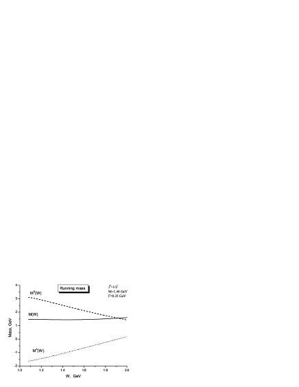
Figure 1: Running mass and width and their components for resonance of positive parity.

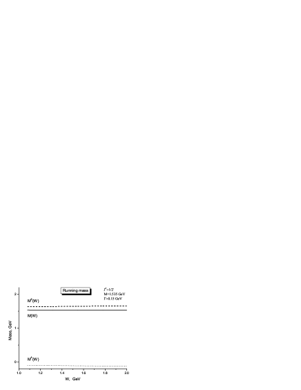
Figure 2: Running mass and width and their components for resonance of negative parity.

References

- (1) G.Breit and E.P.Wigner. Phys. Rev. 49 (1936) 519.
- (2) W.-M. Yao et al. Review of Particle Physics J.Phys. G33 (2006) 1.
- (3) V.Pascalutsa and O.Sholten. Nucl. Phys. A593 (1995) 658.
- (4) G.Lopez Castro and A.Mariano. Nucl. Phys. A697 (2002) 440.
- (5) L.Alvarez-Ruso et al. Phys. Rev. C70 (2004) 015207.
- (6) A.V.Anisovich et al. Eur. Phys. J. A24 (2005) 111.
- (7) G.Höhler. Pion-Nucleon Scattering, Landoldt-Börnstein Vol. I/9b2, edited by H.Schopper, Springer Verlag, 1983.
- (8) R.E.Cutkosky et. al. Phys. Rev. D49 (1979) 2839.
- (9) R.A.Arndt et. al. Phys. Rev. C69 (2004) 035213.
- (10) P. Maris and C. D. Roberts. Int. J. Mod. Phys. E12 (2003) 297.
- (11) A. Sirlin. Phys. Rev. Lett. 67 (1991) 2127.
- (12) M.Passera and A. Sirlin. Phys. Rev. D58 (1998) 113010.
- (13) A.E. Kaloshin and V.P. Lomov. Mod.Phys.Lett. A19 (2004) 135.
- (14) A.E. Kaloshin and V.P. Lomov. Yad. Fiz. 69 (2006) 563.
- (15) P. van Nieuwenhuizen. Phys. Rep. 68 (1981) 189.
- (16) S.Gasiorovicz. Elementary particle physics. John Wiley&Sons Inc., New York-London-Sydney, 1966.
- (17) C.L. Korpa and A.E.L. Dieperink. Phys. Rev. C70 (2004) 015207.