Chiral extrapolation of lattice data for $B$-meson decay constant

Abstract

The $B$-meson decay constant $f_{B}$ has been calculated from unquenched lattice QCD in the unphysical region. For extrapolating the lattice data to the physical region, we propose a phenomenological functional form based on the effective chiral perturbation theory for heavy mesons, which respects both the heavy quark symmetry and the chiral symmetry, and the non-relativistic constituent quark model which is valid at large pion masses. The inclusion of pion loop corrections leads to nonanalytic contributions to $f_{B}$ when the pion mass is small. The finite-range regularization technique is employed for the resummation of higher order terms of the chiral expansion. We also take into account the finite volume effects in lattice simulations. The dependence on the parameters and other uncertainties in our model are discussed.

1 Introduction

An accurate determination of the Cabibbo - Kobayashi - Maskawa (CKM) matrix of the Standard Model and tests of its consistency and unitarity constitute an important part of current research in particle physics. Among the most important matrix elements is the $B$-meson decay constant $f_{B}$, which is needed to determine the CKM matrix elements such as $V_{td}$. Lattice Quantum Chromodynamics (QCD) simulations, which provide a way to determine $f_{B}$ from the first principles of QCD, are of fundamental importance since the determination of the $B$-meson decay constant still remains beyond the reach of experiment.

In Ref.Alan , the authors studied $f_{B}$ extensively from full and partially quenched lattice QCD. In the simulations they applied two actions, the unquenched gauge configurations by the MILC CollaborationC.B and the improved staggered light quark actionS.N , for simulating the light quarks ($u,d,s$). The non-relativistic QCD (NRQCD) formalism was used to treat the heavy quarks ($c,b$)B.A . The lattice data were obtained in the region where the mass of light quark is about in the region 20 MeV $\sim$ 80 MeVAlan (corresponding to the pion mass between around 250 MeV and 500 MeV), which is larger than its physical value. The light quark masses in these simulations are much closer to the physical region than previous work. This makes it possible to reduce the uncertainty from chiral extrapolation. To extrapolate the lattice data to the physical region the staggered chiral perturbation theory was employed in Refs.Alan C.A .

In QCD, when the heavy quark mass goes to infinity, the strong interaction can be described by the heavy quark effective theory (HQET)Mark98 , which contains the heavy quark symmetry $SU(2)_{f}\times SU(2)_{s}$. On the contrary, when the masses of light quarks $(u,d,s)$ approach zero, the strong interaction has $SU(3)_{L}\times SU(3)_{R}$ chiral symmetry which is spontaneously broken to the $SU(3)_{V}$ subgroup, leading to eight pseudoscalar Goldstone bosons. When the light quark mass (or the pion mass) is small enough, the effective chiral LagrangianMark93 containing the chiral and heavy quark symmetries may be applied, based on power counting which is the foundation of chiral perturbation theory. The authors of Ref.thomas found that the regime where power counting may be applied is $0\leq m_{\pi}\leq 180$ MeV by analyzing the chiral extrapolation of the nucleon mass to fourth-order in the expansion and demanding the accuracy of the prediction for the nucleon mass to be one percent. This regime is beyond the reach of current lattice simulations. In order to extrapolate lattice data which are outside the power-counting regime, the so-called finite-range regularization (FRR) technique is proposedthomas ; adelaide ; guo1 ; guo2 , in which a finite-range cutoff (which is physically of order of the inverse size of the pion source) in the momentum integrals of the pion loop diagrams is introduced for the resummation of the chiral expansion. It has been shown strictly that FRR is mathematically equivalent to minimal subtraction schemes such as dimensional regularization to any finite orderthomas . Furthermore, the model dependence associated with the shape of the regulator is at one percent level in the range $0\leq m_{\pi}\leq 1$ GeV, which is well outside the power-counting regime. In the present work we will adopt FRR while applying the effective chiral Lagrangian to extrapolate the lattice data for the $B$-meson decay constant since these data are outside the power-counting regime.

The constituent quark model has been shown to work quite well although it is a very simple model where Quantum Chromodynamics is not employed. At large pion masses, we employ the non-relativistic constituent quark model to fit the lattice data. In fact, for all the hadron properties (such as heavy meson masses and decay constants) which have been calculated in lattice QCD, the lattice data vary slowly and smoothly when the light quark mass is larger than 60 MeV or so. This is characteristic of constituent quark behavior and suggests that in this region the constituent quark model should be most appropriatecloet . In other words, the hadron properties vary as a function of the constituent quark mass in the region of heavier quark mass. It has been shown that the constituent quark model is consistent with the modeling of QCD via the Dyson-Schwinger Equation in ladder-rainbow truncation when the quark mass is largeguo2 . Obviously the lattice data at large light quark masses in Ref.Alan appear in the region where the constituent quark model is suitable to be employed. Consequently, we apply the constituent quark model in this large quark mass region and then analytically continue the hadron properties to the physical mass regime in a manner consistent with chiral symmetry, because of which nonanalytic terms are involved.

In Ref.Alan , the authors extrapolated the lattice data for the quantity $\Phi_{B}$ ($\Phi_{B}=f_{B}\sqrt{m_{B}}$) with the following formula:

$$\Phi_{B}=c_{0}(1+\Delta+{\rm analytic\;\;terms}),$$ (1)

where $c_{0}$ is a constant associated with the axial-vector current which destroys $B$ meson, $\Delta$ is the term encompassing the chiral logarithms, and the analytic term is linear in the light quark mass. It is obvious that when Eq.(1) is used for extrapolating the lattice data, power counting in chiral perturbation theory has been applied when the light quark mass (or the pion mass) is small and the term linear in the light quark mass has been assumed when the light quark mass is large. However, as mentioned before, the lattice data appear in the light quark mass range 20 MeV $\sim$ 80 MeV (or the pion mass range 250 MeV $\sim$ 500 MeV). This is already outside the regime where power counting can be applied ($0\leq m_{\pi}\leq 180$) for small pion masses and inside the regime where the constituent quark model is most appropriate for large pion masses. Therefore, based on our above argument, instead of using the form like Eq.(1) to extrapolate the lattice data for the $B$-meson decay constant, we adopt FRR when applying chiral Lagrangian and the constituent quark model at small and large pion masses, respectively.

The outline of this paper is as follows. We will give a brief review for the chiral perturbation theory for heavy mesons in Sect. 2. In Sect. 3, we will propose a functional form for extrapolating the lattice data to the physical region based on the effective chiral perturbation theory for heavy mesons and the constraints from the constituent quark model at large pion masses. Then in Sect. 4, we will present our fits to the lattice data and give the numerical results. Finally, a summary and discussion will be given in Sect. 5.

2 Chiral perturbation theory for heavy mesons

The chiral perturbation theory for heavy mesons, which describes the interactions of mesons containing a single heavy quark with light pseudoscalar bosons, contains both the heavy quark symmetry $SU(2)_{f}\times SU(2)_{s}$ and the chiral symmetry $SU(3)_{L}\times SU(3)_{R}$, provided $m_{Q}\rightarrow\infty$ and $m_{q}\rightarrow 0$ ($Q$ = $c$ or $b$, $q=u,d,s$ ), respectivelyMark93 .

The pseudoscalar Goldstone bosons are incorporated in a $3\times 3$ unitary matrix

$$\Sigma={\rm exp}\left(\frac{2iM}{f_{\pi}}\right),$$ (2)

where $f_{\pi}$ is the pion decay constant, $f_{\pi}\simeq 131$ MeV, and

$$M=\left(\begin{array}[]{ccc}\frac{1}{\sqrt{2}}\pi^{0}+\frac{1}{\sqrt{6}}\eta&\pi^{+}&K^{+}\\ \pi^{-}&-\frac{1}{\sqrt{2}}\pi^{0}+\frac{1}{\sqrt{6}}\eta&K^{0}\\ K^{-}&\bar{K}^{0}&-\sqrt{\frac{2}{3}}\eta\\ \end{array}\right).$$ (6)

While discussing the strong interaction between heavy mesons and light pseudoscalar mesons it is convenient to introduce

$$\xi=\sqrt{\Sigma}.$$ (7)

Under a chiral $SU(3)_{L}\times SU(3)_{R}$ transformation,

$$\Sigma \rightarrow L\Sigma R^{\dagger},$$

$$\xi \rightarrow L\xi U^{\dagger}=U\xi R^{\dagger},$$

where the unitary matrix $U$ is a complicated nonlinear function of $L$, $R$ and the pseudoscalar Goldstone boson fields.

In order to describe the interactions of the Goldstone bosons with the heavy mesons containing $Q\bar{q}^{a}$ (here $a=1,2,3$ for $u,d,s$ quarks, respectively), it is convenient to introduce a $4\times 4$ matrix $H_{a}$ given in Ref.Mark93 ,

$$H_{a}=\frac{1+\hbox to0.0pt{/\hss}v}{2}(P_{a\mu}^{*}\gamma^{\mu}-P_{a}\gamma_{5}),$$ (8)

where $P_{a}$ and $P^{*}_{a\mu}$ are the field operators that destroy a heavy pseudoscalar meson ($P_{a}$) and a heavy vector meson ($P^{*}_{a}$) with four-velocity $v$, respectively. $P_{a\mu}^{*}$ satisfies the constraint as the following:

$$v^{\mu}P_{a\mu}^{*}=0.$$ (9)

Under $SU(3)_{L}\times SU(3)_{R}$ transformation,

$$H_{a}\rightarrow H_{b}U_{ba}^{\dagger},$$

and under the heavy quark spin transformation,

$$H_{a}\rightarrow SH_{a}.$$

Defining

$$\bar{H}_{a}=\gamma^{0}H_{a}^{\dagger}\gamma^{0},$$ (10)

we have

$$\bar{H}_{a}=(P_{a\mu}^{\dagger}\gamma^{\mu}+P_{a}^{\dagger}\gamma_{5})\frac{1+\hbox to0.0pt{/\hss}v}{2}.$$ (11)

It is convenient to introduce a vector field $V_{ab}^{\mu}$,

$$V_{ab}^{\mu}=\frac{1}{2}(\xi^{\dagger}\partial^{\mu}\xi+\xi\partial^{\mu}\xi^{\dagger})_{ab},$$ (12)

and an axial-vector field $A_{ab}^{\mu}$,

$$A_{ab}^{\mu}=\frac{i}{2}(\xi^{\dagger}\partial^{\mu}\xi-\xi\partial^{\mu}\xi^{\dagger})_{ab},$$ (13)

to establish the Lagrangian for the chiral perturbation theory.

The most general form of the effective Lagrangian density, which is invariant under the heavy quark symmetry and the chiral symmetry and should be invariant under Lorentz and parity transformations as well, is as followsMark93 :

$${\cal L}=-{\rm Tr}[\bar{H}_{a}iv_{\mu}(D^{\mu}H)_{a}]+g{\rm Tr}(\bar{H}_{a}H_{b}\gamma_{\mu}A^{\mu}_{ba}\gamma_{5}),$$ (14)

where $g$ is the coupling constant describing the interaction between heavy mesons and Goldstone bosons, which contains information about the interaction at the quark level. So it cannot be fixed from the chiral perturbation theory for heavy mesons, but should be determined by experiments. The covariant derivative in Eq.(13) is defined as

$$(D^{\mu}H)_{a}=\partial^{\mu}H_{a}-H_{b}V_{ba}^{\mu}.$$ (15)

Then we have the following explicit form for the interaction of heavy mesons with Goldstone bosons after substituting Eqs.(8)(11)(12)(13) into Eq.(14):

$${\rm Tr}[\bar{H}_{a}iv_{\mu}V^{\mu}_{ba}H_{b}]+g{\rm Tr}(\bar{H}_{a}H_{b}\gamma_{\mu}A^{\mu}_{ba}\gamma_{5})$$

$$= \frac{i}{f_{\pi}^{2}}v^{\mu}[M,\partial_{\mu}M]_{ba}(P_{a\nu}^{*{\dagger}}P_{b}^{*\nu}-P_{a}^{\dagger}P_{b})$$ (16)

$$-\frac{2g}{f_{\pi}}(P_{a\mu}^{*{\dagger}}P_{b}\partial^{\mu}M_{ba}+P_{a}^{\dagger}P_{b\mu}^{*}\partial^{\mu}M_{ba}$$

$$+i\epsilon^{\mu\nu\rho\sigma}P_{a\rho}^{*{\dagger}}P_{b\sigma}^{*}v_{\nu}\partial_{\mu}M_{ba}),$$

where $O(M^{3})$ terms are ignored.

Taking the mass difference between $P_{a}$ and $P_{a}^{*}$ into account, the following term has to be added into $\cal{L}$ in Eq.(13):

$$\frac{\lambda_{2}}{m_{Q}}{\rm Tr}{\bar{H}}_{a}\sigma^{\mu\nu}H_{a}\sigma_{\mu\nu},$$ (17)

where $\lambda_{2}$ is a constant containing interaction information at the quark level.

So the propagators for heavy pseudoscalar and vector mesons are

$$\frac{i}{2(v\cdot p+\frac{3}{4}\triangle)}$$ (18)

and

$$\frac{-i(g_{\mu\nu}-v_{\mu\nu})}{2(v\cdot p-\frac{1}{4}\triangle)}$$ (19)

respectively, where $p$ is the residual momentum of the heavy meson. In Eqs.(17)(18)

$$\triangle=-\frac{8\lambda_{2}}{m_{Q}},$$ (20)

which is the mass difference between vector and pseudoscalar heavy mesons.

3 Formulas for the extrapolation of the $B$-meson decay constant

The decay constant of a pseudoscalar heavy meson, $P$, is defined by

$$\langle 0|J^{\mu}|P\rangle=if_{P}m_{P}v^{\mu},$$ (21)

where the axial-vector current is

$$J^{\mu}=\bar{q}\gamma^{\mu}(1-\gamma_{5})Q,$$ (22)

$q$ denotes $u,d$ light quarks and $Q$ represents heavy quarks $c,b$.

The current in Eq.(21) can be written in the low energy chiral theory asMark92

$$J_{a}^{\mu}=(\frac{i\alpha}{2}){\rm Tr}[\gamma^{\mu}(1-\gamma_{5})H_{b}\xi_{ba}^{\dagger}],$$ (23)

where $\alpha$ is a parameter.

Substituting Eq.(5) into Eq.(22), we have the following explicit form for the current $J_{a}^{\mu}$:

$$J_{a}^{\mu}=i\alpha(P_{b}^{*\mu}-v^{\mu}P_{b})\xi_{ba}^{\dagger}.$$ (24)

We make a Taylor expansion for $M$ and omit $O(\frac{1}{f_{\pi}^{3}})$ terms. This leads to the following expression for $J^{\mu}_{a}$:

$$J_{a}^{\mu}=i\alpha(P_{b}^{*\mu}-v^{\mu}P_{b})[\delta_{ba}-\frac{i}{f_{\pi}}(M)_{ba}-\frac{1}{2f_{\pi}^{2}}(M^{2})_{ba}].$$ (25)

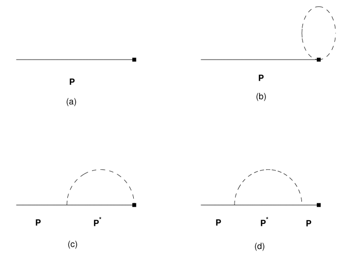
Figure 1: Heavy meson decay constant to one pion loop order. The black squares represent the weak current in Eq.(22), and dashed lines denote the pion.

The diagrams for the heavy meson decay constant to one pion loop order from Eqs.(15)(24) are shown in Fig. 1. We can see that there are three diagrams for one pion loop corrections to the pseudoscalar heavy meson decay constant.

From Fig. 1(a), it is easy to obtain

$$\alpha=-f_{P}^{(0)}\sqrt{m_{P}},$$ (26)

where $f_{P}^{(0)}$ is the heavy pseudoscalar meson decay constant at the tree level where pion loop corrections are not taken into account.

Fig. 1(b) represents the pion loop correction from the axial current $J_{a}^{\mu}$ itself. It can be expressed as

$$f_{P}^{(b)}=-\frac{3i}{4f_{\pi}^{2}}f_{P}^{(0)}\int\frac{{\rm d^{4}}k}{(2\pi)^{4}}\frac{1}{k^{2}-m_{\pi}^{2}},$$ (27)

where $k$ is the four momentum of the pion in the loop and $m_{\pi}$ is the pion mass which is not necessary to be its physical mass.

Choosing the contour in the lower half complex plane of $k_{0}$, in which there is only one pole for $k_{0}$, we have the following result after integrating over $k_{0}$:

$$f_{P}^{(b)}=-\frac{3}{8f_{\pi}^{2}}f_{P}^{(0)}\int\frac{{\rm d^{3}}k}{(2\pi)^{3}}\frac{1}{w_{k}},$$ (28)

where $w_{k}=\sqrt{|\vec{k}|^{2}+m_{\pi}^{2}}$ .

Fig. 1(c) vanishes because of the identity

$$v^{\mu}(g_{\mu\nu}-v_{\mu}v_{\nu})=0.$$

The contribution of Fig. 1(d) to the matrix element in Eq.(21) is

$$\frac{9ig^{2}}{2(v\cdot p+\frac{3}{4}\bigtriangleup)f_{\pi}^{2}}f_{P}^{(0)}X$$ (29)

multiplied by $im_{P}v^{\mu}$, where the self-energy contribution is proportional to

$$X=\frac{1}{3}\int\frac{{\rm d^{4}}k}{(2\pi)^{4}}\frac{k^{2}-(v\cdot k)^{2}}{[v\cdot(p-k)-\frac{1}{4}\triangle](k^{2}-m_{\pi}^{2})}.$$ (30)

Since $v\cdot p$ is a Lorentz scalar, we are free to choose the special frame in which the heavy meson is at rest: $v^{0}=1,\vec{v}=0$. Choosing the same contour in the evaluation of the integral as before, we have (details are given in Ref.guo1 )

$$X=\frac{i}{6}\int\frac{{\rm d^{3}}k}{(2\pi)^{3}}\frac{|\bf k|^{2}}{w_{k}(w_{k}-\delta)},$$ (31)

where $\delta=v\cdot p-\frac{1}{4}\triangle$.

The contribution to $f_{P}$ from the one-loop wave function renormalization, $f_{P}^{(d)}$, can be obtained from the derivative of $X$ with respect to $v\cdot p$:

$$\frac{1}{2}\frac{\partial X}{\partial v\cdot p}|_{v\cdot p=-\frac{3}{4}\Delta}.$$ (32)

Then we have

$$f_{P}^{(d)}=-\frac{3g^{2}}{8f_{\pi}^{2}}f_{P}^{(0)}\int\frac{{\rm d^{3}}k}{(2\pi)^{3}}\frac{|\bf k|^{2}}{w_{k}(w_{k}-\delta)^{2}}.$$ (33)

Adding all the contributions from the diagrams in Fig. 1, we have the following expression for $f_{P}$:

$$f_{P}=f_{P}^{(0)}+f_{P}^{(b)}+f_{P}^{(d)},$$ (34)

where the first term represents the contribution at the tree level, and the other two come from one pion loop corrections.

When the light quark mass is near the chiral limit, pion loop corrections give the dominate contributions to $f_{P}$; on the contrary, pion loop contributions vanish in the limit $m_{\pi}\rightarrow\infty$. In order to extrapolate the lattice data, we also have to know the behavior of $f_{P}$ at the large pion mass. Based on the non-relativistic constituent quark model, it is known for a long time that, up to logarithmic corrections, $f_{P}$ obeys the asymptotic scaling law when the constitute quark masses are very large:

$$f_{P}\sqrt{m_{P}}={\rm constant}.$$ (35)

The above behavior is also obtained in the Dyson-Schwinger Equation approachM.A .

Therefore, it is convenient to extrapolate $f_{P}\sqrt{m_{P}}$ instead of $f_{P}$. Then we only need to introduce a constant parameter while fitting the lattice data in the region where $m_{\pi}$ is large.

Based on the above argument, we propose the following functional form for extrapolating the heavy meson decay constant from unphysical region to the physical limit:

$$\Phi_{P}=\sqrt{m_{P}}(f_{P}^{(0)}+f_{P}^{(b)}+f_{P}^{(d)})+b_{P}^{\prime},$$ (36)

where

$$\Phi_{P}=f_{P}\sqrt{m_{P}},$$ (37)

and $b_{P}^{\prime}$ is a parameter.

It is convenient to define the following new parameters:

$$a_{P} = \sqrt{m_{P}}f_{P}^{(0)},$$

$$b_{P} = \sqrt{m_{P}}f_{P}^{(0)}+b_{P}^{\prime}.$$ (38)

So we have the following explicit functional form for extrapolating the lattice data:

$$\Phi_{P}=a_{P}\sigma^{\chi}_{P}+b_{P},$$ (39)

where

$$\sigma^{\chi}_{P} = -\frac{3}{8f_{\pi}^{2}}\int\frac{{\rm d^{3}}k}{(2\pi)^{3}}\frac{1}{w_{k}}$$ (40)

$$-\frac{3g^{2}}{8f_{\pi}^{2}}\int\frac{{\rm d^{3}}k}{(2\pi)^{3}}\frac{|\bf k|^{2}}{w_{k}(w_{k}-\delta)^{2}}$$

from Eqs.(27)(32), and $a_{P}$ and $b_{P}$ are the parameters to be determined by fitting the lattice data.

As mentioned in Introduction, for extrapolating the lattice data which are outside the power-counting regime, the FRR technique can be used for the resummation of the chiral expansion. In FRR, a finite-range cutoff in the momentum integrals of the pion loop diagrams is introduced. We choose two different approaches for evaluating the integrals in Eq.(39). One is the sharp-cutoff form, $\theta(\Lambda-|\vec{k}|)$, and the other is the dipole form, $\Lambda^{4}/(\Lambda^{2}+|\vec{k}|^{2})^{2}$. Both of them make the integrals converge. When the pion mass is greater than the cutoff $\Lambda$, which characterizes the finite size of the source of the pion, the Compton wavelength of the pion is smaller than that of the source and pion loop contributions are suppressed as powers of $\Lambda/m_{\pi}$. Obviously the dipole form is more realistic. Since the leading nonanalytic contribution of pion loops is only associated with the infrared behavior of the integrals in Eq.(39), it does not depend on the details of $\Lambda$.

Since the lattice simulations are performed on a finite volume grid, the finite size effects should be taken into accountD.B . In the finite periodic volume, the available momenta $k$ are discrete:

$$k=\frac{2\pi n}{aL},$$ (41)

where $L$ is the number of lattice sites in the $x,y,z$ direction, and the integer $n$ is in the following range:

$$-\frac{L}{2}<n\leq\frac{L}{2}.$$ (42)

Since the pion momenta on the finite lattice volume are discrete, we should take this into account by replacing the continuous integral over $k$ in Eq.(40) with a discrete sum over $k$,

$$\int{\rm d^{3}}k\approx(\frac{2\pi}{aL})^{3}\sum_{k_{x},k_{y},k_{z}}\ ,$$ (43)

where the discrete momenta $k_{x}$, $k_{y}$, $k_{z}$ are given in Eq.(40). From Ref.Alan1 , the volume of lattice simulation is $20^{3}\times 64$, corresponding to $L=20$. The smallest momentum allowed on the lattice is $2\pi/aL$.

4 Extrapolation of lattice data for pseudoscalar heavy meson decay constant

Lattice gauge theory is the only quantitative tool currently available to calculate nonperturbative phenomena in QCD from first principles. Quark vacuum polarization is the most expensive ingredient in lattice QCD simulations, especially when quark masses are very small, as in the case of $u$ and $d$ quarks. The MILC Collaboration has established unquenched gauge configuration, which contains three flavors of light sea quarks to include the effects of realistic quark vacuum polarizationC.B . This staggered quark discretization of QCD has several advantages, which are offset by the fact that staggered quarks always come in groups of four identical flavors. In Refs.S.N C.A C.A1 , the Kogut-Susskind action with improved flavor and rotational symmetry suitable for dynamical fermion simulations is constructed. At tree level, the action has no couplings of quarks to gluons with a transverse momentum component $\pi/a$. So the flavor symmetry violating terms in the action are completely removed at tree level. Then the rotational symmetry is improved by introducing the Naik term. Finally, an extra five link staple is introduced in order to cancel errors of ${\cal O}(a^{2}g^{2})$ from the fattening. The result action is called $Asq$ action. It can be further improved by tadpole improvement, leading to $Asqtad$, which is an order ${\cal O}(a^{4},a^{2}g^{2})$ accurate fermion action.

The authors of Ref.Alan studied the $B$-meson decay constant employing the MILC Collaboration unquenched gauge configuration, and light sea quarks are represented by the highly improved staggered quark action. The good chiral properties of the latter action allow for a much smoother chiral extrapolation to the physical region. The $b$ quark inside $B$ meson is treated only as the valence quark in simulations because its effect in the sea should be suppressed by inverse powers of the $b$ quark massM.N . NRQCD lattice action was used to deal with the valence $b$ quark, which has been developed over many years B.A G.P C.T . The $b$ quark is non-relativistic inside its bound state, hence a non-relativistic expansion of the QCD action is appropriate which accurately handles scales of the order of typical momenta and kinetic energies inside these states.

Some lattice data of $\Phi_{B}$ are obtained in Ref.Alan from full or partially quenched QCD. The coarse lattice spacing $a$ is around 0.12fm. In the case of full QCD, dynamical light quark masses are chosen as $m_{q}/m_{s}$ = 0.125, 0.175, 0.25 and 0.5, where $m_{s}$ is the strange quark mass, corresponding to $\Phi_{B}$ = 0.516(5)(15), 0.519(5)(15), 0.517(8)(15) and 0.540(5)(15) (in unit of GeV^3/2), respectively (the errors in the first parentheses are statistical and the second come from lattice spacing uncertainties). In the case of partially quenched QCD, dynamical light quark masses are chosen as $m_{q}/m_{s}$ = 0.125 and 0.5, corresponding to $\Phi_{B}$ = 0.506(5)(14), and 0.547(5)(15) (in unit of GeV^3/2), respectively. Two values of $\Phi_{B}$ in the case of fine lattices with $a$ being around 0.087fm have also been accumulated, where the staggered valence light propagators created by the Fermilab Collaboration were used to treat the light quarks.

We choose to extrapolate the coarse data (full and partially quenched) since the number of the fine data is only two. If we used the fine data, the uncertainty of the fitted results due to the error in the lattice data would be too large. Explicit lattice simulations show that over the rang of mass of interest to us, where the pion mass is not constrained by the chiral limit, $m_{\pi}$ is proportional to $m_{q}$C.A2 .

In our model, there are two parameters, $a_{P}$ and $b_{P}$, to be fixed in Eq.(39). These parameters are related to $g$, $\lambda_{2}$ and $\Lambda$. $g$ and $\lambda_{2}$ represent the interaction at the quark level and cannot be determined from the chiral perturbation theory for heavy mesons. From the experimental data for the decay width for $D\rightarrow D^{*}\pi$, we have the variation of $g$ between 0.51 and 0.67A.Ana . From Eq.(16), $\lambda_{2}$ is related to the mass splitting between a heavy vector meson and a heavy pseudoscalar meson. Based on the experimental data for $B$ mesons, the value of $\lambda_{2}$ should be around $-0.03GeV^{2}$. To see the dependence on $\lambda_{2}$ in our fits, we let $\lambda_{2}$ vary between $-0.03GeV^{2}$ and $-0.02GeV^{2}$. We let $\Lambda$ vary between $0.4GeV$ and $0.6GeV$, considering the scale of the finite size of the pion sourceguo1 guo2 . The two parameters, $a_{P}$ and $b_{P}$, are determined by the least squares fitting method in our fit.

We first extrapolate the full QCD data. In this case, the uncertainties of the parameters $a_{B}$ and $b_{B}$ are around 90% and 10%, respectively, due to the errors in the lattice data. The large uncertainty of $a_{B}$, associated with the chiral correction term, is due to the lack of the lattice data near the physical region. In Table 1, the fitted results in Columns 3 and 5 (Columns 2 and 4) correspond to the case where the finite lattice volume effects are (not) taken into account. We can see that the difference between these two cases is not very large.

The fitted result for $f_{B}$ is obtained from Column 5 in Table 1, where the dipole form factor is used and the correction from the discretization of the pion momentum is considered:

$$f_{B}=214.2\pm 13.3\pm 0.8MeV,$$ (44)

where the first uncertainty is from the errors in the lattice data, and the second is from the variation of parameters ($g,\lambda_{2},\Lambda$) in our model.

If we use the sharp cutoff scheme, the fitted result for $f_{B}$ is

$$f_{B}=215.1\pm 15.8\pm 4.1MeV.$$ (45)

We then extrapolate the full QCD data together with the two partially quenched data (although, in principle, one should use quenched chiral Lagrangian to extrapolate these two data). As expected, we find that the uncertainties which are due to the errors in the lattice data for $a_{B}$, $b_{B}$, and the extrapolated $B$-meson decay constant are all reduced since the number of the lattice data increases (see Table 2).

The fitted result for $f_{B}$ is obtained from Column 5 in Table 2, where the dipole form factor is used and the correction from the discretization of the pion momentum is considered as before:

$$f_{B}=209.4\pm 9.7\pm 1.0MeV,$$ (46)

where the first uncertainty is from the errors in the lattice data, and the second is from the variation of parameters ($g,\lambda_{2},\Lambda$) in our model.

If we use the sharp cutoff scheme, the fitted result for $f_{B}$ is

$$f_{B}=210.5\pm 11.4\pm 5.7MeV.$$ (47)

It can be seen that the extrapolated results for the $B$-meson decay constant are consistent with each other in the above two extrapolation cases and in the two cutoff schemes if we consider the uncertainties of the extrapolated results. We can also see that the uncertainties due to variations of our model parameters in the dipole scheme, which is more realistic, are smaller than those in the sharp cutoff scheme.

5 Summary and discussion

It is known that the strong interactions are constrained by the heavy quark symmetry when the heavy quark mass goes to infinity, and by the chiral symmetry when the light quark mass approaches zero. The chiral perturbation theory can be applied when the light quark mass (or the pion mass) is small enough. In the region where the light quark mass is bigger than about 60 MeV, the non-relativistic constituent quark model is appropriate. Base on these, we propose a phenomenological functional form to extrapolate the lattice data for the $B$-meson decay constant to the physical region, combining the chiral perturbation theory and the non-relativistic constituent quark model.

We evaluate pion loop contributions when $m_{\pi}$ is small with the aid the chiral perturbation theory for heavy mesons. This leads to correct nonanalytic chiral behavior of $f_{B}$ in the chiral limit. Since the lattice data for the $B$-meson decay constant is outside the power-counting regime, instead of simply using the chiral logarithms as done in Ref.Alan , we employ the finite-range regularization technique in order to resum higher order terms of the chiral expansion. At large pion masses, we introduce a constant parameter to fit the lattice data for $\Phi_{B}$ (which appear in the region where the constituent quark model is suitable to be applied) based on the non-relativistic constituent quark model. This is also different from the term linear in light quark mass used in Ref.Alan . It has been pointed out that in large pion mass region, the extrapolation based on the constituent quark model is more reasonable than the simple linear extrapolationguo2 . The finite lattice volume effects are taken into account by replacing the continuous integral with a discrete sum. In our fit, the two parameters are determined by the least squares fitting method.

In Ref.Alan , the lattice data for the $B$-meson decay constant (both full QCD and partially quenched data) are extrapolated based on the staggered chiral perturbation theory with power counting being used. The result of the extrapolated $B$ decay constant at the physical pion mass is

$$f_{B}=0.216(9)(19)(4)(6)GeV,$$ (48)

where the errors, from left to right, are statistics plus scale plus chiral extrapolations, higher order matching, discretization, and relativistic corrections plus $m_{b}$ tuning respectively.

It can be seen that the central values for the extrapolated $B$-meson decay constant in Eqs.(46)(47) are smaller than that in Eq.(48). However, because of the large uncertainties due to the errors in the lattice data and the model parameters etc. the extrapolated $B$-meson decay constant in our work is still consistent with that in Ref.Alan .

Now we discuss the uncertainties in our model. We have three parameters, $\lambda_{2}$, $g$ and $\Lambda$, where the first two are related to the color-magnetic-moment operator at order $1/m_{Q}$ in HQET and the interaction between heavy mesons and Goldstones in chiral perturbation theory, respectively. Appropriate ranges for them (obtained from the comparison with the experimental data) are used in our fit process. We did not take into account the $O(a^{2})$ contributions in the Kogut-Susskind action, which could give 7% corrections to our resultAlan . In our approach, sea quark mass is not extrapolated. Usually quenched lattice QCD gives about 90% contribution to physical quantities, hence sea quark contribution is at about 10% level. Therefore, one expects the uncertainty from sea quark extrapolation is about $1\sim 2$%. Taking these into account, our extrapolated result in Eqs.(44-47) may have another 8% uncertainty. In our future work we will investigate these issues carefully in order to reduce these uncertainties.

Acknowledgements. This work was supported in part by Special Grants for ”Jing Shi Scholar” of Beijing Normal University and by National Nature Science Foundation of China Project No. 10675022.

Table 1: Fitting parameters, the fitted results in the sharp-cutoff and the dipole schemes and the (relative) uncertainties caused by the errors in the lattice data in the full QCD case are shown. The variations of the values in the second to the fifth columns are due to the variations of the parameters in our model.

Form factor	sharp cutoff		dipole
Volume	infinite	finite	infinite	finite
$a_{B}$ (GeV3/2)	0.3644-0.9395	0.3759-1.0388	0.5068-1.1943	0.5098-1.1965
$\triangle a_{B}/a_{B}$ (%)	89.30-91.38	89.36-91.62	88.72-89.83	88.75-89.84
$b_{B}$ (GeV3/2)	0.5715-0.5928	0.5712-0.5910	0.6017-0.6368	0.5981-0.6275
$\triangle b_{B}/b_{B}$ (%)	7.86-10.58	7.69-1.05	11.80-15.88	11.34-14.81
$\Phi$ (GeV3/2)	0.4944-0.4994	0.4844-0.5035	0.4971-0.5000	0.4900-0.4936
$\triangle\Phi$ (GeV3/2)	0.0227-0.0275	0.0195-0.0364	0.0221-0.0248	0.0277-0.0305
$\triangle\Phi/\Phi$ (%)	4.54-5.57	3.87-7.52	4.42-4.99	5.61-6.23
$f_{B}$ (GeV)	0.2153-0.2175	0.2110-0.2193	0.2165-0.2178	0.2134-0.215
$\triangle f_{B}$ (GeV)	0.0099-0.0120	0.0085-0.0159	0.0096-0.0108	0.0120-0.0133
$\triangle f_{B}/f_{B}$ (%)	4.54-5.57	3.87-7.52	4.42-4.99	5.61-6.23

Table 2: Fitting parameters, the fitted results in the sharp-cutoff and the dipole schemes and the (relative) uncertainties caused by the errors in the lattice data in the case where both the full QCD and partially quenched QCD data are fitted are shown. The variations of the values in the second to the fifth columns are due to variation of the parameters in our model.

Form factor	sharp cutoff	sharp cutoff	dipole	dipole
Volume	infinite	finite	infinite	finite
$a_{B}$ (GeV3/2)	0.5160-1.3369	0.5075-1.4148	0.6810-1.6116	0.6851-1.6146
$\triangle a_{B}/a_{B}$ (%)	49.47-52.91	47.35-47.78	47.23-47.43	47.24-47.44
$b_{B}$ (GeV3/2)	0.5944-0.6238	0.5878-0.6160	0.6295-0.6758	0.6247-0.6633
$\triangle b_{B}/b_{B}$ (%)	6.22-8.69	5.31-7.16	8.03-10.66	7.72-9.98
$\Phi_{B}$ (GeV3/2)	0.4839-0.4910	0.4707-0.4968	0.4971-0.5000	0.4788-0.4835
$\triangle\Phi_{B}$ (GeV3/2)	0.0177-0.0217	0.0144-0.0262	0.0163-0.0182	0.0202-0.0223
$\triangle\Phi_{B}/\Phi_{B}$ (%)	3.62-4.48	2.90-5.58	3.32-3.72	4.18-4.66
$f_{B}$ (GeV)	0.2105-0.2137	0.2048-0.2162	0.2163-0.2176	0.2084-0.2104
$\triangle f_{B}$ (GeV)	0.0077-0.0094	0.0063-0.0114	0.0071-0.0079	0.0088-0.0097
$\triangle f_{B}/f_{B}$ (%)	3.62-4.48	2.90-5.58	3.32-3.72	4.18-4.66

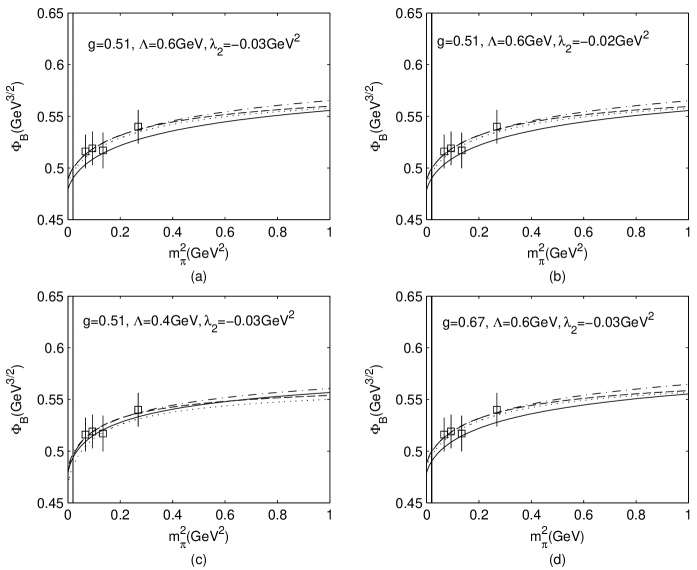
Figure 2: Extrapolation of the full QCD lattice data for the $B$-meson decay constant. Dashed line (dotted line) corresponds to the sharp cutoff scheme and infinite (finite) volume; dash-dot line (solid line) corresponds to the dipole scheme and infinite (finite) volume. The vertical solid line corresponds to the physical pion mass.

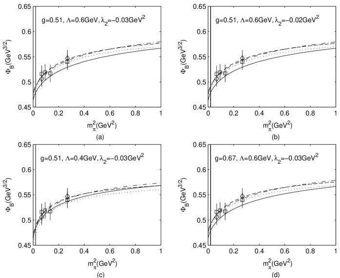
Figure 3: Extrapolation of both the full QCD and partially quenched QCD lattice data (which are represented by squares and diamonds respectively) for the $B$-meson decay constant. Dashed line (dotted line) corresponds to the sharp cutoff scheme and infinite (finite) volume; dash-dot line (solid line) corresponds to the dipole scheme and infinite (finite) volume. The vertical solid line corresponds to the physical pion mass.

References

- (1) A. Gray et al., Phys. Rev. Lett. 95, 212001 (2005).
- (2) C. Bernard et al., Phys. Rev. D64, 054506 (2001).
- (3) S. Naik, Nucl. Phys. B316, 238 (1989); G. P. Lepage, Phys. Rev. D59, 074501 (1999); K. Orifinos et al., Phys. Rev. D60, 054503 (1999); C. Bernard et al., Phys. Rev. D58, 014503 (1998); ibid. 61, 111502 (2000).
- (4) B. A. Thacker and G. Peter Lepage, Phys. Rev. D43, 196 (1991).
- (5) C. Aubin and C. Bernard, Nucl. Phys. B, Proc. Suppl. 140, 491 (2005).
- (6) N. Isgur and M. B. Wise, Phys. Lett. B232, 113 (1989), B237, 527 (1990); H. Georgi, Phys. Lett. B264, 447 (1991); see also M. Neubert, Phys. Rep. 245, 259 (1994) for the review.
- (7) M. B. Wise, Phys. Rev. D45, 2188 (1992).
- (8) D. B. Leinweber, A. W. Thomas, and R. D. Young, Phys. Rev. Lett. 92, 242002 (2004); Nucl. Phys. A755, 59c (2005).
- (9) D. B. Leinweber, A. W. Thomas, K. Tsushima, and S. V. Wright, Phys. Rev. D61, 074502 (2000); D. B. Leinweber, D. H. Lu, and A. W. Thomas, Phys. Rev. D60, 034014 (1999); E. J. Hackett-Jones, D. B. Leinweber, and A. W. Thomas, Phys. Lett. B489, 143 (2000); D. B. Leinweber and A. W. Thomas, Phys. Rev. D62, 074505 (2000); W. Detmold, W. Melnitchouk, and A. W. Thomas, Eur. Phys. J. C13, 1 (2001); W. Detmold, W. Melnitchouk, J. W. Negele, D. B. Renner, and A. W. Thomas, Phys. Rev. Lett. 87, 172001 (2001); E. J. Hackett-Jones, D. B. Leinweber, and A. W. Thomas, Phys. Lett. B494, 89 (2000).
- (10) X.-H. Guo and A. W. Thomas, Phys. Rev. D65, 074019 (2002); ibid. 67, 074005 (2003).
- (11) X.-H. Guo, P. C. Tandy, and A. W. Thomas, Few Body Syst. 38, 17 (2006).
- (12) I. C. Cloet, D. B. Leinweber, and A. W. Thomas, Phys. Rev. C65, 062201(R) (2002).
- (13) B. Grinstein and M. B. Wise, Nucl. Phys. B380, 369 (1992).
- (14) M. A. Ivanov, Yu. L. Kalinovsky, P. Maris, and C. D. Roberts, Phys. Lett. B416, 29 (1998).
- (15) D. B. Leinweber, A. W. Thomas, K. Tsushima, and S. V. Wright, Phys. Rev. D64, 094502 (2001).
- (16) A. Gray, I. Allison, C. T. H. Davies, E. Gulez, G. P. Lepage, J. Shigemitsu, and M. Wingate, Phys. Rev. D72, 094507 (2005).
- (17) C. Aubin et al., Phys. Rev. D70, 031504 (2004).
- (18) M. Nobes, [arXiv: hep-lat/0501009].
- (19) G. P. Lepage et al., Phys. Rev. D46, 4052 (1992).
- (20) C. T. H. Davies, K. Hornbostel, A. Langnau, G. P. Lep- age, A. Lidsey, J. Shigemitsu, and J. Sloan, Phys. Rev. D50, 6963 (1994).
- (21) MILC Collaboration (C. Aubin et al.), Phys. Rev. D70, 114501 (2004).
- (22) CELO Collaboration (A. Anastassov et al.), Phys. Rev. D65, 032003 (2002).