x Two-Loop Ultrasoft Running of the $O(v^{2})$ QCD Quark Potentials

Abstract

The two-loop ultrasoft contributions to the next-to-leading logarithmic (NLL) running of the QCD potentials at order $v^{2}$ are determined. The results represent an important step towards the next-to-next-to-leading logarithmic (NNLL) description of heavy quark pair production and annihilation close to threshold.

I Introduction

The measurement of the line-shape of the total top-antitop quark production cross section in the threshold region $\sqrt{s}\approx 2m_{t}$ is one of the major tasks within the top quark physics program at the ILC. The most prominent quantity to be measured is the top quark mass, and one expects an improvement in precision of $m_{t}$ by about an order of magnitude to mass measurements based on reconstruction obtained at the Tevatron and the LHC thresholdscan .

To obtain a meaningful theoretical description of the nonrelativistic threshold dynamics it is required to systematically sum the so-called Coulomb singular terms $\propto(\alpha_{s}/v)^{n}$ in a systematic nonrelativistic expansion, $v$ being the relative velocity of the top quarks. This task is achieved by means of effective theories based on nonrelativistic QCD (NRQCD) BBL . In this approach, however, sizeable logarithmic terms $\propto(\alpha_{s}\ln v)^{n}$ are not systematically accounted for, which leads to rather large normalization uncertainties of the cross section line-shape. The next-to-next-to-leading order predictions in this “fixed-order” approach were estimated to have a normalization uncertainty of order $20\%$ synopsis . These normalization uncertainties do not affect the top mass measurement, which primarily depends on the c.m. energy where the cross section rises, but they render measurements of other quantities such as the top total width or the top quark couplings impossible. To match the statistical uncertainties, that are expected for these quantities, a theoretical precision of the cross section normalization of at least $3\%$ would be required.

In Refs. HMST (see also Ref. PinedaSigner ) it was demonstrated that the summation of logarithmic $(\alpha_{s}\ln v)^{n}$ terms, using renormalization-group-improved perturbation theory, can significantly reduce the normalization uncertainties of the threshold cross section. Concerning QCD effects the renormalization group improved LL (leading-logarithmic) and NLL order predictions of the threshold cross section are completely known, but no full NNLL order prediction exists at present. The full NNLL order prediction is, however, required to obtain a reliable estimate of the remaining theoretical normalization uncertainties.

The missing ingredient is the NNLL running of the Wilson coefficient of the leading order effective current, that describes production and annihilation of a nonrelativistic $t\bar{t}$ pair in a S-wave spin-triplet state (${}^{3}S_{1}$). Adopting the label notation from vNRQCD LMR ; HoangStewartultra the current has the form

$${\bf J}_{1,\bf p}=\psi_{\mathbf{p}}^{\dagger}\,\mbox{\boldmath$\sigma$}(i\sigma_{2})\chi_{-\mathbf{p}}^{*}\,,$$ (1)

where $\psi_{\mathbf{p}}$ and $\chi_{\mathbf{p}}$ annihilate top and antitop quarks with three-momentum $\mathbf{p}$, respectively, and where color indices have been suppressed. The current does not have a LL anomalous dimension because there is no one-loop vertex diagram in the effective theory that contains UV divergences associated with the current ${\bf J}_{1,\bf p}$. Such UV divergences arise at NLL order from insertions of the NNLL kinetic energy operators and from insertions of the NNLL order potentials LMR . The corresponding computations were carried out in Refs. amis ; amis2 ; Pineda:2001et ; HoangStewartultra and are completed. Using the conventions from HoangStewartultra the resulting NLL order renormalization group equation for the Wilson coefficient $c_{1}$ of the current has the form (${\bf S}^{2}=2$)

$$\nu\frac{\partial}{\partial\nu}\ln[c_{1}(\nu)] = -\>\frac{{\cal V}_{c}^{(s)}(\nu)}{16\pi^{2}}\bigg{[}\frac{{\cal V}_{c}^{(s)}(\nu)}{4}+{\cal V}_{2}^{(s)}(\nu)+{\cal V}_{r}^{(s)}(\nu)+{\bf S}^{2}\>{\cal V}_{s}^{(s)}(\nu)\bigg{]}$$ (2)

$$+\>\alpha_{s}^{2}(m\nu)\,\bigg{[}\frac{C_{F}}{2}(C_{F}-2\,C_{A})\bigg{]}+\alpha_{s}^{2}(m\nu)\,\bigg{[}3{\cal V}_{k1}^{(s)}(\nu)+2{\cal V}_{k2}^{(s)}(\nu)\bigg{]}\,,$$

where $\nu$ is the vNRQCD velocity renormalization parameter that is conveniently used to parametrize the correlation between soft and ultrasoft dynamical scales within the renormalized effective theory LMR . The analogous evolution equation for currents describing pairs of quarks and colored scalars in any angular momentum and spin state (${}^{2s+1}L_{J}$) were derived recently in Ref. HoangRuiz2 . In Eq. (2) the term ${\cal V}_{c}^{(s)}$ is the Wilson coefficient of the Coulomb potential $\propto 1/\mathbf{k}^{2}$, and ${\cal V}_{2}^{(s)}$ and ${\cal V}_{r}^{(s)}$ are the coefficients of the ${\cal O}(v^{2})$ potentials with the momentum structure $1/m^{2}$ and $(\mathbf{p}^{2}+{\mathbf{p}^{\prime}}^{2})/(2m^{2}\mathbf{k}^{2})$, respectively, $m$ being the heavy quark mass. The coefficients ${\cal V}_{k1,k2}^{(s)}$ are from the so-called non-Abelian potentials that scale like $1/(m|\mathbf{k}|)$, and ${\cal V}_{s}^{(s)}$ is the coefficient of the spin-dependent potential that can contribute for spin triplet S-wave states. The superscripts ${(s)}$ refer to the color singlet state of the quark pair.

At NNLL order there are two kinds of contributions to the evolution of $c_{1}$ that have to be accounted for. The first kind arises from three-loop vertex diagrams that come from insertions of subleading soft matrix element corrections to the potentials and from insertions of potentials with additional exchange of ultrasoft gluons. The corresponding computations were carried out in Ref. 3loop . These effects are referred to as the non-mixing contributions as they affect the evolution of $c_{1}$ directly. The second kind of contributions arises from the subleading evolution of the potential Wilson coefficients that appear in the NLL order renormalization group equation shown in Eq. (2). They are referred to as the mixing contributions as they affect the evolution of $c_{1}$ indirectly. Except for the coefficient of the Coulomb potential ${\cal V}_{c}^{(s)}$ Pineda:2001ra ; HoangStewartultra and for the spin-dependent potential ${\cal V}_{s}^{(s)}$ Penin:2004xi no complete determination for the subleading evolution exists at present. The analysis of the three-loop (non-mixing) terms in Ref. 3loop revealed that the contributions involving the exchange of ultrasoft gluons are more than an order of magnitude larger than those arising from soft matrix element insertions and are as large as the known NLL contributions. The reason is related to the larger size of the ultrasoft coupling $\alpha_{s}(m\nu^{2})$ and to a rather large coefficient multiplying the ultrasoft contributions. These large ultrasoft contributions are responsible for an uncertainty in the normalization of the most up-to-date threshold cross section prediction of at best $6\%$ HoangEpiphany , which is quite far from the required precision. (See also Ref. PinedaSigner for an alternative analysis without NNLL non-mixing effects.) The corresponding effects of the soft matrix element corrections are only at the level of several per mille. From this analysis it is reasonable to assume that the ultrasoft effects, which form a gauge-invariant subset, also dominate the mixing contributions. This assumption is also consistent with the results for the NLL evolution of the coefficient ${\cal V}_{s}^{(s)}$ Penin:2004xi , which is dominated by soft effects, since the ultrasoft gluon coupling to heavy quarks is spin-independent at this order, and which was found to have a very small numerical effect as well Penin:2004ay . From the parametric point of view this can be understood from the fact that ultrasoft effects can affect the coefficients of the spin-dependent potentials only indirectly through mixing via potential loop divergences, since at this order the coupling of ultrasoft gluons to heavy quarks are spin-independent. For the coefficient of spin-dependent potentials this leads to ultrasoft NLL terms $\propto\alpha_{S}^{2}(\alpha_{U}\ln v)^{n}$, where $\alpha_{S}$ and $\alpha_{U}$ are the strong coupling at the soft and ultrasoft scales, respectively. These terms are parametrically suppressed compared to ultrasoft NLL terms $\propto\alpha_{S}\alpha_{U}(\alpha_{U}\ln v)^{n}$ that can affect the spin-independent potential coefficients through two-loop ultrasoft loop diagrams. We can therefore expect that ultrasoft effects are dominating the higher order evolution of the spin-independent potentials.

In this work we determine as a first step the two-loop ultrasoft contributions to the NLL anomalous dimensions of the spin-independent potentials ${\cal V}_{2}$ and ${\cal V}_{r}$. The outline of this work is as follows: in Sec. II we briefly review the effective theory setup used for our work and in Sec. III we present our results. Sec. IV contains a brief numerical analysis and Sec. V the conclusion.

II Theoretical Setup

The vNRQCD Lagrangian basically consists of three parts LMR ; HoangStewartultra ,

$${\cal L}_{\rm vNRQCD}\>=\>{\cal L}_{u}\>+\>{\cal L}_{p}\>+\>{\cal L}_{s}\,,$$ (3)

containing kinetic terms and ultrasoft interactions, potential interactions and interactions involving soft degrees of freedom, respectively. The “ultrasoft part” ${\cal L}_{u}$ has the form

$${\cal L}_{u}=\sum_{\mathbf{p}}\bigg{\{}\psi_{\mathbf{p}}^{\dagger}\!\bigg{[}iD^{0}-\frac{\left({\bf p}\!-\!i{\bf D}\right)^{2}}{2m}+\frac{\mathbf{p}^{4}}{8m^{3}}+\ldots\!\bigg{]}\!\psi_{\mathbf{p}}+(\psi\!\to\!\chi,\,T\!\to\!\bar{T})\bigg{\}}\!-\frac{1}{4}G^{\mu\nu}G_{\mu\nu}+\ldots,\!$$ (4)

where the ultrasoft gauge-covariant derivative reads $D^{\mu}=\partial^{\mu}+ig_{U}A^{\mu}(x)$ and $g_{U}$ is the strong coupling at the ultrasoft scale $m\nu^{2}$. The terms describe besides the propagation of the heavy quarks their interaction with ultrasoft gluons. The “potential part” ${\cal L}_{p}$ describes the potential quark-antiquark interactions and reads

$${\cal L}_{p} = -\sum_{\mathbf{p},{\mathbf{p}^{\prime}}}V_{\alpha\beta\lambda\tau}\left({\mathbf{p}},{{\mathbf{p}^{\prime}}}\right)\ \psi_{{\mathbf{p}^{\prime}}\alpha}^{\dagger}\>\psi_{\mathbf{p}\,\beta}\>\chi_{-{\mathbf{p}^{\prime}}\lambda}^{\dagger}\>\chi_{-\mathbf{p}\,\tau}+\ldots\,,$$ (5)

where $\alpha,\beta,\lambda,\tau$ are color indices and

$$V_{\alpha\beta\lambda\tau}({\mathbf{p}},{\mathbf{p}^{\prime}}) = (T^{A}_{\alpha\beta}\otimes\bar{T}^{A}_{\lambda\tau})\,\bigg{[}\frac{{\cal V}_{c}^{(T)}}{\mathbf{k}^{2}}+\frac{{\cal V}_{k}^{(T)}\pi^{2}}{m|{\mathbf{k}}|}+\frac{{\cal V}_{r}^{(T)}({\mathbf{p}^{2}+\mathbf{p}^{\prime 2}})}{2m^{2}\mathbf{k}^{2}}+\frac{{\cal V}_{2}^{(T)}}{m^{2}}+\ldots\bigg{]}$$ (6)

$$+\,(1_{\alpha\beta}\otimes\bar{1}_{\lambda\tau})\,\bigg{[}\frac{{\cal V}_{c}^{(1)}}{\mathbf{k}^{2}}+\frac{{\cal V}_{k}^{(1)}\pi^{2}}{m|{\mathbf{k}}|}+\frac{{\cal V}_{r}^{(1)}({\mathbf{p}^{2}+\mathbf{p}^{\prime 2}})}{2m^{2}\mathbf{k}^{2}}+\frac{{\cal V}_{2}^{(1)}}{m^{2}}+\ldots\bigg{]}$$

with $\mathbf{k}={\mathbf{p}^{\prime}}-\mathbf{p}$. The spin-dependent ${\cal O}(v^{2})$ potentials have not been written out in Eq. (6), since they will not be relevant in this work. One can convert the potentials from the basis formed by the two ${\bf 3}\otimes{\bf\bar{3}}$ color structures $1\otimes\bar{1}$ and $T^{A}\otimes\bar{T}^{A}$ into the more physical color singlet/octet basis by

$$\left[\begin{array}[]{c}V_{\rm singlet}\cr V_{\rm octet}\end{array}\right]=\left[\begin{array}[]{ccc}1&&-C_{F}\cr 1&&\frac{1}{2}C_{A}-C_{F}\cr\end{array}\right]\left[\begin{array}[]{c}V_{1\otimes 1}\cr V_{T\otimes T}\end{array}\right]\,.$$ (13)

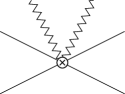
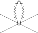
a)               b)               c)

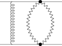
Figure 1: a) Operator ${\cal O}_{2i}$, b) operator ${\cal O}_{2i}$ with soft lines closed to a loop, c) diagram with soft and ultrasoft loop contributing to potential counterterms.

In the soft sector of the theory there are 6-field operators needed for the description of soft Compton scattering off quark-antiquark potentials (see Fig. 1a). As was pointed out in Ref. HoangStewartultra these operators have zero matching conditions at the hard scale $\nu=1$ and contribute to the ultrasoft renormalization of the ${\cal O}(v^{2})$ potentials. The operators have the structure

$${\cal O}_{2\varphi}^{(\sigma),(T)} = {g_{S}^{4}}\>\>(\psi_{\mathbf{p}^{\prime}}^{\dagger}\>\Gamma^{(\sigma),(T)}_{\varphi,\psi}\>\psi_{\mathbf{p}})\>(\chi_{-\mathbf{p}^{\prime}}^{\dagger}\>\Gamma^{(\sigma),(T)}_{\varphi,\chi}\>\chi_{-\mathbf{p}})\ (\overline{\varphi}_{-q}\>\Gamma_{\varphi}^{(\sigma),(T)}\>\varphi_{q})\,,$$

$${\cal O}_{2A}^{(\sigma),(T)} = {g_{S}^{4}}\>\>(\psi_{\mathbf{p}^{\prime}}^{\dagger}\>\Gamma^{(\sigma),(T)}_{A,\psi}\>\psi_{\mathbf{p}})\>(\chi_{-\mathbf{p}^{\prime}}^{\dagger}\>\Gamma^{(\sigma),(T)}_{A,\chi}\>\chi_{-\mathbf{p}})\ (A^{\mu}_{-q}\>\Gamma_{A,\mu\nu}^{(\sigma),(T)}\>A^{\nu}_{q})\,,$$ (14)

$$\ {\cal O}_{2c}^{(\sigma),(T)} = {g_{S}^{4}}\>\>(\psi_{\mathbf{p}^{\prime}}^{\dagger}\>\Gamma^{(\sigma),(T)}_{c,\psi}\>\psi_{\mathbf{p}})\>(\chi_{-\mathbf{p}^{\prime}}^{\dagger}\>\Gamma^{(\sigma),(T)}_{c,\chi}\>\chi_{-\mathbf{p}})\ (\bar{c}_{-q}\>\Gamma_{c}^{(\sigma),(T)}\>c_{q})\,,$$ (15)

where $\varphi_{q},A^{\mu}_{q}$ and $c_{q}$ denote soft quarks, gluons and ghosts respectively, $g_{S}$ is the strong coupling at the soft scale $m\nu$ and $\sigma$ is the order at which the operators contribute in the $v$-counting. For the explicit form of the the $\Gamma$’s we refer to Ref. HoangStewartultra (see also Ref. HoangRuiz1 ). The superscript $(T)$ refers to the color structure $(T^{A}\otimes\bar{T}^{A})$ that arises upon closing the two soft lines (see Fig. 1b). There is another set of such operators, which are not displayed, having the superscript $(1)$, that refers to the color structure $(1\otimes\bar{1})$ that arises upon closing the two soft lines. As was shown in Ref. HoangStewartultra , closing the two respective two soft lines for the leading $\sigma=0$ operators, one obtains a structure for the one-loop four-quark matrix elements that is identical to the one-loop soft-matrix element corrections to the Coulomb potential. Moreover, the Wilson coefficients of the $\sigma=2$ operators become nonzero for $\nu<1$ from ultrasoft UV divergences (and the associated pull-up terms HoangStewartultra ; zerobin ) in higher-order corrections to the vNRQCD matrix elements describing Compton scattering off a quark-antiquark pair. The coefficients of these operators are directly affected by ultrasoft gluon corrections to this process. Through the UV divergences that arise upon closing the two soft lines they mix into the potential coefficients ${\cal V}_{2}^{(s)}$ and ${\cal V}_{r}^{(s)}$. Using the counting mentioned above the contributions from these mixing contributions to the evolution of ${\cal V}_{2}^{(s)}$ and ${\cal V}_{r}^{(s)}$ are parametrically suppressed compared to the contributions from the two-loop ultrasoft diagrams that renormalize these potentials directly. For the purpose of this work we need the $\sigma=2$ operators that have the form

$${\cal O}_{2k}^{(2),(1)} = \frac{\mathbf{k}^{2}}{m^{2}}\,\sum_{i}{\cal O}_{2i}^{(0),(1)}\,,\quad{\cal O}_{2k}^{(2),(T)}\,=\,\frac{\mathbf{k}^{2}}{m^{2}}\,\sum_{i}{\cal O}_{2i}^{(0),(T)}\,,\quad$$

$${\cal O}_{2p}^{(2),(1)} = \frac{(\mathbf{p}^{2}+\mathbf{p}^{\prime\,2})}{m^{2}}\,\sum_{i}{\cal O}_{2i}^{(0),(1)}\,,\quad{\cal O}_{2p}^{(2),(T)}\,=\,\frac{(\mathbf{p}^{2}+\mathbf{p}^{\prime\,2})}{m^{2}}\,\sum_{i}{\cal O}_{2i}^{(0),(T)}\,,$$ (16)

which have the Wilson coefficients $C^{(1,T)}_{2k}$ and $C^{(1,T)}_{2p}$, respectively. We note that the mixing effects of these operators lead to numerical effects for ${\cal V}_{2}^{(s)}$ and ${\cal V}_{r}^{(s)}$ that are substantially smaller than those from the two-loop ultrasoft diagrams that renormalize ${\cal V}_{2}^{(s)}$ and ${\cal V}_{r}^{(s)}$ directly. We include them because their contribution leads to a rather simple form for the two-loop ultrasoft corrections to ${\cal V}_{2}^{(s)}$ and ${\cal V}_{r}^{(s)}$ we determine in this work and also in order to illustrate the size of the contributions not considered in this work.

All fields, couplings and Wilson coefficients in the above Lagrangian are to be understood as bare quantities. For the renormalized ones we chose the usual conventions in $d=4-2\epsilon$ dimensions ($\mu_{S}=m\nu,\mu_{U}=m\nu^{2}$):

$$\begin{array}[]{ll}V=\mu_{S}^{2\epsilon}(V_{R}\!+\!\delta V)\,,&C_{2i}=C_{2i}^{R}\!+\!\delta C_{2i}\,,\\ g_{U}\,=\,\mu_{U}^{\epsilon}\,g_{U}^{R}\,,&g_{S}\,=\,\mu_{S}^{\epsilon}\,g_{S}^{R}\,,\\ \psi_{\mathbf{p}}=Z^{1/2}_{\psi,\mathbf{p}}\;\psi_{\mathbf{p}}^{R}\,,&Z_{\psi,\mathbf{p}}=1\!+\!\delta Z_{\psi,\mathbf{p}}\,,\;\;(\psi\to\chi),\\ A^{\mu}=Z_{A}^{1/2}\>A_{R}^{\mu}\;,&Z_{A}=1\!+\!\delta Z_{A}\,.\end{array}$$ (17)

For convenience, we will drop the index $R$ throughout this paper and only deal with ${\overline{\rm MS}}$ renormalized quantities in the following.

III Results

In general the counter term of the potentials induced by ultrasoft renormalization takes the form

$$\delta\vec{V}=A\,\vec{V}+\vec{C}\,,$$ (18)

where $\delta\vec{V}$, $\vec{V}$ and $\vec{C}$ are 2-vectors and A is a $2\times 2$ matrix in the $(1\otimes\bar{1}$, $T^{A}\otimes\bar{T}^{A})$ space,

$$\vec{V}=\left[\begin{array}[]{c}V_{1\otimes 1}\cr V_{T\otimes T}\end{array}\right]\,.$$ (19)

From Eq. (18) one can deduce the general form of the renormalization group equations for the potentials:

$$\nu\frac{d}{d\nu}\,\vec{V} = -2\epsilon\,\vec{V}-(1+A)^{-1}\big{(}\,2\epsilon\,\vec{C}\,+\,\nu\frac{d}{d\nu}\,\vec{C}\,+\,(\nu\frac{d}{d\nu}A)\,\vec{V}\,\big{)}\,.$$ (20)

The full one-loop results for $A$ and $\vec{C}$ can be found in Ref. amis ; HoangStewartultra . For the ultrasoft contributions at the two-loop level we define different classes of (divergent) two-loop diagrams in Feynman gauge contributing to the matrix $A$:
class topology insertions/vertices (e.g. $\psi_{\mathbf{p}}^{\dagger}\,gA^{0}\psi_{\mathbf{p}}$,  $\psi_{\mathbf{p}}^{\dagger}\,g\frac{\mathbf{p}\cdot\mathbf{A}}{m}\psi_{\mathbf{p}}$,  $\psi_{\mathbf{p}}^{\dagger}\frac{\mathbf{p}\cdot\mathbf{\nabla}}{m}\psi_{\mathbf{p}}$,  etc.) order 1 Fig. 2a four $gA^{0}$ vertices ${\cal O}(v^{0})$ 2 Fig. 2b one gluon selfenergy insertion and two $gA^{0}$ vertices ${\cal O}(v^{0})$ 3 Fig. 2a two $gA^{0}$ and two $g\frac{\mathbf{p}\cdot\mathbf{A}}{m}$ vertices ${\cal O}(v^{2})$ 4 Fig. 2b one gluon selfenergy insertion and two $g\frac{\mathbf{p}\cdot\mathbf{A}}{m}$ vertices ${\cal O}(v^{2})$ 5 Fig. 2a two $gA^{0}$ vertices and two insertions of the $\frac{\mathbf{p}\cdot\mathbf{\nabla}}{m}$ operator on the internal quark lines ${\cal O}(v^{2})$ 6 Fig. 2b one gluon selfenergy insertion, two $gA^{0}$ vertices and two insertions of the $\frac{\mathbf{p}\cdot\mathbf{\nabla}}{m}$ operator on the internal quark lines ${\cal O}(v^{2})$ 7 Fig. 2b one gluon selfenergy insertion, one $gA^{0}$, one $g\frac{\mathbf{p}\cdot\mathbf{A}}{m}$ vertex and one insertion of the $\frac{\mathbf{p}\cdot\mathbf{\nabla}}{m}$ operator on the internal quark lines ${\cal O}(v^{2})$ 8 Fig. 2c one triple gluon interaction, one $gA^{0}$ and two $g\frac{\mathbf{p}\cdot\mathbf{A}}{m}$ vertices ${\cal O}(v^{2})$ 9 Fig. 2c one triple gluon interaction, two $gA^{0}$, one $g\frac{\mathbf{p}\cdot\mathbf{A}}{m}$ vertex and one insertion of the $\frac{\mathbf{p}\cdot\mathbf{\nabla}}{m}$ operator on the internal quark lines ${\cal O}(v^{2})$

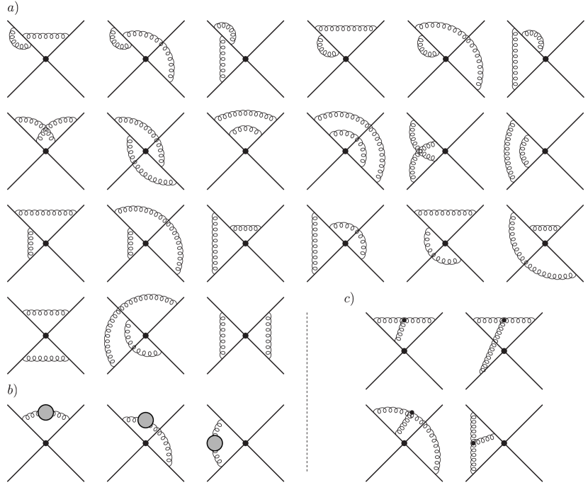
Figure 2: 2-loop topologies: a) “Abelian”, b) with gluon selfenergy, c) “Non-Abelian”. Left-right and up-down mirror graphs are not shown.

To each of these classes there is a corresponding class of diagrams, which contribute to the heavy quark wavefunction counterterm $\delta Z_{\psi,\mathbf{p}}$, with the same type and number of vertices and insertions. The results for the different contributions to $\delta Z_{\psi,\mathbf{p}}$ after subtraction of the respective one-loop subdivergencies are shown in Tab. 1. The table also shows an example diagram for each of the classes.

class	example diagram	contribution to $\delta Z_{\psi,\mathbf{p}}$	order
1		$\frac{C_{F}(C_{F}-C_{A})\alpha_{U}^{2}}{8\pi^{2}\epsilon^{2}}+\frac{C_{A}C_{F}\alpha_{U}^{2}}{8\pi^{2}\epsilon}$	${\cal O}(v^{0})$
2		$-\frac{C_{F}(5C_{A}-4\,Tn_{f})\alpha_{U}^{2}}{32\pi^{2}\epsilon^{2}}+\frac{C_{F}(13C_{A}-8\,Tn_{f})\alpha_{U}^{2}}{48\pi^{2}\epsilon}$	${\cal O}(v^{0})$
3		$-\frac{C_{F}(C_{F}-C_{A})\mathbf{p}^{2}\alpha_{U}^{2}}{4\,m^{2}\pi^{2}\epsilon^{2}}-\frac{C_{A}C_{F}\mathbf{p}^{2}\alpha_{U}^{2}}{4\,m^{2}\pi^{2}\epsilon}$	${\cal O}(v^{2})$
4		$\frac{C_{F}(15\,C_{A}-12\,Tn_{f})\mathbf{p}^{2}\alpha_{U}^{2}}{288\,m^{2}\pi^{2}\epsilon^{2}}-\frac{C_{F}(46\,C_{A}-32\,Tn_{f})\mathbf{p}^{2}\alpha_{U}^{2}}{288\,m^{2}\pi^{2}\epsilon}$	${\cal O}(v^{2})$
5		$\frac{C_{F}(C_{F}-C_{A})\mathbf{p}^{2}\alpha_{U}^{2}}{4\,m^{2}\pi^{2}\epsilon^{2}}+\frac{C_{A}C_{F}\mathbf{p}^{2}\alpha_{U}^{2}}{4\,m^{2}\pi^{2}\epsilon}$	${\cal O}(v^{2})$
6		$-\frac{C_{F}(75\,C_{A}-60\,Tn_{f})\mathbf{p}^{2}\alpha_{U}^{2}}{288\,m^{2}\pi^{2}\epsilon^{2}}+\frac{C_{F}(110\,C_{A}-64\,Tn_{f})\mathbf{p}^{2}\alpha_{U}^{2}}{288\,m^{2}\pi^{2}\epsilon}$	${\cal O}(v^{2})$
7		$\frac{C_{F}(15\,C_{A}-12\,Tn_{f})\mathbf{p}^{2}\alpha_{U}^{2}}{72\,m^{2}\pi^{2}\epsilon^{2}}-\frac{C_{F}(16\,C_{A}-8\,Tn_{f})\mathbf{p}^{2}\alpha_{U}^{2}}{72\,m^{2}\pi^{2}\epsilon}$	${\cal O}(v^{2})$
8		0	${\cal O}(v^{2})$
9		0	${\cal O}(v^{2})$

Table 1: Contributions to $\delta Z_{\psi,\mathbf{p}}$ at ultrasoft 2-loop level $(\alpha_{U}\equiv\alpha_{s}(m\nu^{2}))$.

The result for the ultrasoft two-loop contributions to the matrix $A$ reads:

$$A = {\textstyle\frac{\alpha_{U}^{2}}{m^{2}}\left(-\frac{11C_{A}-4Tn_{f}}{72\,\pi^{2}\epsilon^{2}}+\frac{(-3\pi^{2}+47)C_{A}-10Tn_{f}}{108\,\pi^{2}\epsilon}\right)}\left[\begin{array}[]{ll}C_{F}\mathbf{k}^{2}&-C_{1}\mathbf{k}^{2}\\ -\mathbf{k}^{2}&\left(C_{F}+\frac{C_{d}}{4}-\frac{3C_{A}}{4}\right)\mathbf{k}^{2}+C_{A}(\mathbf{p}^{2}+{\mathbf{p}^{\prime}}^{2})\end{array}\right]$$ (23)

$$+ {\textstyle\frac{\alpha_{U}^{2}}{m^{2}}\frac{C_{A}}{6\epsilon}}\left[\begin{array}[]{ll}0&C_{1}\left(\mathbf{k}^{2}-\frac{9}{4}(\mathbf{p}^{2}+{\mathbf{p}^{\prime}}^{2})\right)\\ -\frac{1}{4}(\mathbf{p}^{2}+{\mathbf{p}^{\prime}}^{2})-\mathbf{k}^{2}&-\frac{5}{8}(C_{A}-4C_{F})(\mathbf{p}^{2}+{\mathbf{p}^{\prime}}^{2})\end{array}\right],$$ (26)

where $C_{1}=\frac{1}{2}C_{F}(C_{A}-2C_{F})$ and $C_{d}=8C_{F}-3C_{A}$.
Here and in the following $\alpha_{U}\equiv\alpha_{s}(m\nu^{2})$ and $\alpha_{S}\equiv\alpha_{s}(m\nu)$. The expression in Eq. (26) represents the main result of this work. It is an important cross check that the ${\cal O}(\alpha_{U}^{2}\,v^{0})$ terms vanish identically as a consequence of ultrasoft gauge invariance. In addition, our result for the ultrasoft two-loop ${\cal O}(v^{0})$ wave function renormalization constant agrees with the ${\cal O}(\alpha_{s}^{2}\,m^{0})$ heavy quark wave function renormalization constant in heavy quark effective theory (HQET), see e.g. Ref. Grozin:2000cm . There is agreement since the purely ultrasoft sector of NRQCD is closely related to HQET Manohar:1997qy . Furthermore we find that all ${\cal O}(v^{2})$ terms cancel in our result for the ultrasoft two-loop wave function renormalization constant (see Tab. 1). This cancellation also takes place for the ${\cal O}(v^{2})$ terms at one-loop and is required by consistency since the form of the bilinear heavy quark kinetic terms in Eq. (4) is protected from quantum corrections by reparametrization invariance. As an additional cross check we have also determined all two-loop fermionic $Tn_{f}$ corrections in Coulomb gauge StahlhofenTUM .

From the results obtained in Eq. (26) one can deduce without effort the ultrasoft contributions to the NLL evolution of the Wilson coefficients $C^{(1,T)}_{2k,2p}$, since the additional soft external lines describing soft Compton scattering do not affect the structure of the ultrasoft loop diagrams. Including the two-loop soft terms induced by the pull-up mechanism in analogy to the 1-loop case HoangStewartultra ; zerobin and the corresponding (known) one-loop contributions the respective renormalization group equations read

$$\nu\frac{d}{d\nu}C_{2\mathbf{k}}^{(1,T)}(\nu) = 2\,A^{(1,T)}_{\mathbf{k}}\,(2\alpha_{U}-\alpha_{S})+4\,B^{(1,T)}_{\mathbf{k}}\,(2\alpha_{U}^{2}-\alpha_{S}^{2})\,,$$ (27)

$$\nu\frac{d}{d\nu}C_{2\mathbf{p}}^{(1,T)}(\nu) = 2\,A^{(1,T)}_{\mathbf{p}}\,(2\alpha_{U}-\alpha_{S})+4\,B^{(1,T)}_{\mathbf{p}}\,(2\alpha_{U}^{2}-\alpha_{S}^{2})\,,$$ (28)

where the constants $A^{(1,T)}_{\mathbf{k},\mathbf{p}}$ and $B^{(1,T)}_{\mathbf{k},\mathbf{p}}$ are defined as

$$A^{(1)}_{\mathbf{p}} = 0\,,\qquad\qquad B^{(1)}_{\mathbf{p}}\,=\,-\frac{3}{16}C_{A}C_{F}(C_{A}-2C_{F})\,,$$

$$A^{(T)}_{\mathbf{p}} = \frac{C_{A}}{3\pi}\,,\qquad\quad B^{(T)}_{\mathbf{p}}\,=\,C_{A}\frac{C_{A}(-57\pi^{2}+188)-40Tn_{f}}{432\pi^{2}}+\frac{5C_{A}C_{F}}{12}\,,$$

$$A^{(1)}_{\mathbf{k}} = -\frac{C_{F}(C_{A}-2C_{F})}{6\pi}\,,\qquad B^{(1)}_{\mathbf{k}}\,=\,C_{F}(C_{A}-2C_{F})\frac{C_{A}(21\pi^{2}-47)+10Tn_{f}}{216\pi^{2}}\,,$$

$$A^{(T)}_{\mathbf{k}} = -\frac{C_{A}-2C_{F}}{2\pi}\,,\qquad\qquad B^{(T)}_{\mathbf{k}}\,=\,(C_{A}-2C_{F})\frac{C_{A}(3\pi^{2}-47)+10Tn_{f}}{72\pi^{2}}\,.$$ (29)

The solutions respecting the matching conditions $C^{(1,T)}_{2k,2p}=0$ at $\nu=1$ have the form
($\beta_{0}=\frac{11}{3}C_{A}-\frac{4}{3}Tn_{f}\,,\;\beta_{1}=\frac{34}{3}C_{A}^{2}-4C_{F}Tn_{f}-\frac{20}{3}C_{A}Tn_{f}$):

$$C_{2\mathbf{p}}^{(1,T)}(\nu) = -\frac{4\pi A^{(1,T)}_{\mathbf{p}}}{\beta_{0}}\ln\left(\frac{\alpha_{U}}{\alpha_{S}}\right)+\left[\frac{A^{(1,T)}_{\mathbf{p}}\beta_{1}}{\beta_{0}^{2}}-\frac{8\pi B^{(1,T)}_{\mathbf{p}}}{\beta_{0}}\right](\alpha_{U}-\alpha_{S})\,,$$

$$C_{2\mathbf{k}}^{(1,T)}(\nu) = -\frac{4\pi A^{(1,T)}_{\mathbf{k}}}{\beta_{0}}\ln\left(\frac{\alpha_{U}}{\alpha_{S}}\right)+\left[\frac{A^{(1,T)}_{\mathbf{k}}\beta_{1}}{\beta_{0}^{2}}-\frac{8\pi B^{(1,T)}_{\mathbf{k}}}{\beta_{0}}\right](\alpha_{U}-\alpha_{S})\,.$$ (30)

Upon closing up the two soft gluon, ghost and light quark lines one arrives at the following mixing contributions for $\vec{C}$ in Eq. (18):

$$\vec{C}=-\frac{\alpha_{S}^{2}\,\beta_{0}}{\mathbf{k}^{2}\epsilon}\left[\begin{array}[]{c}C_{2\mathbf{k}}^{(1)}\,\frac{\mathbf{k}^{2}}{m^{2}}\,+\,C_{2\mathbf{p}}^{(1)}\,\frac{\mathbf{p}^{2}+{\mathbf{p}^{\prime}}^{2}}{m^{2}}\\[4.30554pt] C_{2\mathbf{k}}^{(T)}\,\frac{\mathbf{k}^{2}}{m^{2}}\,+\,C_{2\mathbf{p}}^{(T)}\,\frac{\mathbf{p}^{2}+{\mathbf{p}^{\prime}}^{2}}{m^{2}}\end{array}\right].$$ (31)

It is then straightforward to derive the evolution equation for the coefficients ${\cal V}_{2}^{(s)}$ and ${\cal V}_{r}^{(s)}$ of the spin-independent ${\cal O}(v^{2})$ potentials. Using

$$\vec{V}=\left[\begin{array}[]{c}0\\ \frac{{\cal V}_{c}(\nu)}{\mathbf{k}^{2}}\end{array}\right]$$ (32)

with ${\cal V}_{c}(\nu)\,=\,4\,\pi\,\alpha_{s}(m\nu)$ on the RHS of Eq. (20), and including again the soft pull-up terms we obtain

$$\nu\,\frac{d}{d\nu}{\cal V}_{2}^{(1,T)}(\nu) = 8\pi\,A_{\mathbf{k}}^{(1,T)}\,\alpha_{S}\,(2\alpha_{U}-\alpha_{S})+16\pi\,B_{\mathbf{k}}^{(1,T)}\,\alpha_{S}\,(2\alpha_{U}^{2}-\alpha_{S}^{2})-2\,\beta_{0}\,\alpha_{S}^{2}\,C_{\mathbf{k}}^{(1,T)}\,,$$

$$\nu\,\frac{d}{d\nu}{\cal V}_{r}^{(1,T)}(\nu) = 8\pi\,A_{\mathbf{p}}^{(1,T)}\,\alpha_{S}\,(2\alpha_{U}-\alpha_{S})+16\pi\,B_{\mathbf{p}}^{(1,T)}\,\alpha_{S}\,(2\alpha_{U}^{2}-\alpha_{S}^{2})-2\,\beta_{0}\,\alpha_{S}^{2}\,C_{\mathbf{p}}^{(1,T)}\,,\quad$$ (33)

for the dominant NLL ultrasoft contributions. To render the anomalous dimensions finite, we also have to account for UV-divergent contributions from diagrams of the type in Fig. 1c. Note that in Eqs. (33) we have also displayed the LL ultrasoft terms including the respective soft pull-up terms. The full set of the known LL contributions from soft one-loop diagrams amis has not been displayed.

From the previous equations we find the following simple result for the ultrasoft one-loop and two-loop contributions to the evolution of the coefficients ${\cal V}_{2}$ and ${\cal V}_{r}$ up to NLL order:

$$\Big{(}{\cal V}_{2}^{(1,T)}(\nu)\Big{)}_{us} = 4\pi\,\alpha_{s}(m\nu)\,C_{\mathbf{k}}^{(1,T)}(\nu)\,,$$

$$\Big{(}{\cal V}_{r}^{(1,T)}(\nu)\Big{)}_{us} = 8\pi\,\alpha_{s}(m\nu)\,C_{\mathbf{p}}^{(1,T)}(\nu)\,.$$ (34)

The corresponding coefficients for the color singlet potentials read

$$\Big{(}{\cal V}_{2}^{(s)}(\nu)\Big{)}_{us} = 4\pi\,\alpha_{s}(m\nu)\,\Big{(}C_{\mathbf{k}}^{(1)}(\nu)-C_{F}C_{\mathbf{k}}^{(T)}(\nu)\Big{)}\,,$$

$$\Big{(}{\cal V}_{r}^{(s)}(\nu)\Big{)}_{us} = 8\pi\,\alpha_{s}(m\nu)\,\Big{(}C_{\mathbf{p}}^{(1)}(\nu)-C_{F}C_{\mathbf{p}}^{(T)}(\nu)\Big{)}\,.$$ (35)

It is now straightforward to derive from Eq. (2) the two-loop ultrasoft part of the NNLL mixing contributions to the running of the ${}^{3}S_{1}$ current coefficient $c_{1}$ from the coefficients ${\cal V}_{2}^{(s)}$ and ${\cal V}_{r}^{(s)}$. Parametrizing the form of $c_{1}$ as 3loop

$$\ln\Big{[}\frac{c_{1}(\nu)}{c_{1}(1)}\Big{]} = \xi^{\rm NLL}(\nu)+\Big{(}\,\xi^{\rm NNLL}_{\rm m}(\nu)+\xi^{\rm NNLL}_{\rm nm}(\nu)\,\Big{)}+\ldots\,,$$ (36)

where $\xi^{\rm NNLL}_{m}$ and $\xi^{\rm NNLL}_{nm}$ refer to the NNLL mixing and non-mixing contributions, respectively, we find

$$\xi^{\rm NNLL}_{m;2r,{\rm usoft}} = \frac{2\pi C_{F}\beta_{1}}{\beta_{0}^{3}}\,\tilde{A}\,\alpha_{s}^{2}(m)\,\bigg{[}-\frac{7}{4}+\frac{\pi^{2}}{6}+z\left(1-\ln\frac{z}{2-z}\right)+z^{2}\left(\frac{3}{4}-\frac{1}{2}\ln z\right)$$ (37)

$$\hskip 85.35826pt-\ln^{2}\left(\frac{z}{2}\right)+\ln^{2}\left(\frac{z}{2-z}\right)-2\mbox{Li}_{2}\left(\frac{z}{2}\right)\bigg{]}$$

$$+\,\frac{8\pi^{2}C_{F}}{\beta_{0}^{2}}\,\tilde{B}\,\alpha_{s}^{2}(m)\,\Big{[}3-2z-z^{2}-4\ln(2-z)\Big{]}\,,$$

where

$$\tilde{A} = A_{\mathbf{k}}^{(1)}+2A_{\mathbf{p}}^{(1)}-C_{F}\Big{(}A_{\mathbf{k}}^{(T)}+2A_{\mathbf{p}}^{(T)}\Big{)}\,,$$

$$\tilde{B} = B_{\mathbf{k}}^{(1)}+2B_{\mathbf{p}}^{(1)}-C_{F}\Big{(}B_{\mathbf{k}}^{(T)}+2B_{\mathbf{p}}^{(T)}\Big{)}\,,$$

$$z \equiv \left(\frac{\alpha_{s}(m\nu)}{\alpha_{s}(m)}\right)^{\rm LL}\,=\,\bigg{(}1+\frac{\alpha_{s}(m)\beta_{0}}{2\pi}\ln\nu\bigg{)}^{-1}\,.$$ (38)

For completeness we also give the form of the ultrasoft corrections to $\xi^{\rm NLL}$ from ${\cal V}_{2}$ and ${\cal V}_{r}$:

$$\xi^{\rm NLL}_{2r,{\rm usoft}}\>=\>\frac{8\pi^{2}C_{F}}{\beta_{0}^{2}}\,\tilde{A}\,\alpha_{s}(m)\,\Big{[}-1+z+(2-z)\ln(2-z)\Big{]}.$$ (39)

IV Numerical Discussion

In Fig. 3a,b the renormalization parameter $\nu$ dependence of the color singlet coefficients ${\cal V}_{2}^{(s)}$ and ${\cal V}_{r}^{(s)}$ in Eq. (35) is shown at LL order (dashed lines) including all soft and ultrasoft contributions HoangStewartultra ; Pineda:2001ra , and in addition including the full two-loop ultrasoft contributions with (solid lines) and without the mixing contributions from the zero matching operators (dotted lines), that are represented by the respective last terms on the RHS of Eqs. (33). For the heavy quark mass we have adopted $m_{t}=175$ GeV for the application to the top-antitop quark threshold, and $\alpha_{s}(m_{t})=0.1074$.

Figure 3: Renormalization scale dependence of ${\cal V}_{2}^{(s)}$ and ${\cal V}_{r}^{(s)}$. In a), b) the full LL results (soft + ultrasoft) (dashed lines), plus the NLL ultrasoft contributions with (solid lines) and without (dotted lines) the mixing terms is shown. In c), d) only the corresponding ultrasoft results are displayed omitting the known soft LL running. All of them include soft pull-up terms.

To further illustrate the importance of the two-loop ultrasoft contributions we have displayed in Fig. 3c,d the evolution of the coefficients at LL order due to the one-loop ultrasoft contributions alone (dashed lines), and in addition including the two-loop ultrasoft contributions analogous to Figs. 3a and b. Comparing the behavior of the LL order and NLL two-loop ultrasoft contributions in Fig. 3c,d we find that the NLL order corrections are of the same size as the ultrasoft LL order contributions. While for the potential ${\cal V}_{2}^{(s)}$ this is of no concern, since for ${\cal V}_{2}^{(s)}$ the ultrasoft contributions are suppressed by a small overall color factor compared to the soft LL contributions, the result for ${\cal V}_{r}^{(s)}$ shows that the two-loop ultrasoft corrections are indeed anomalously large, similar to the NNLL ultrasoft non-mixing contributions to the evolution of $c_{1}$ determined in Ref. 3loop . From the dotted lines in Fig. 3 we also see that the correction arising from the mixing contributions are numerically small, which is consistent with the parametric counting mentioned in the introduction.

It is also instructive to analyse the impact of the NLL two-loop ultrasoft contributions in ${\cal V}_{2}^{(s)}$ and ${\cal V}_{r}^{(s)}$ on the NNLL evolution of the ${}^{3}S_{1}$ current coefficient $c_{1}$. Evaluating Eq. (37) we find $(\delta c_{1})^{\rm NNLL,mix}_{2,r}\approx\xi^{\rm NNLL}_{m;2r,{\rm usoft}}=(-1.9\%,-0.5\%)$ for $\nu=0.1,0.2$. These corrections lead to a partial compensation of the anomalously large ultrasoft corrections that dominate the NNLL non-mixing contributions to the evolution of $c_{1}$. It remains to be seen whether the two-loop ultrasoft corrections to the evolution of the $1/(m|\mathbf{k}|)$ QCD potentials will lead to a similar effect. We will address this issue in a subsequent work.

V Conclusion

We have determined the two-loop ultrasoft contributions to the NLL order renormalization group equations of the ${\cal O}(v^{2})$ spin-independent QCD potentials ${\cal V}_{2}$ ($1/m^{2}$) and ${\cal V}_{r}$ ($(\mathbf{p}^{2}+{\mathbf{p}^{\prime}}^{2})/(2m^{2}\mathbf{k}^{2})$). We find that the two-loop ultrasoft corrections are larger than the ultrasoft contributions at the one-loop level and lead to a partial cancellation of the anomalously large NNLL ultrasoft non-mixing contributions to the renormalization group evolution of the leading ${}^{3}S_{1}$ current that describes top-antitop pair production at threshold in $e^{+}e^{-}$ annihilation.

- (1) J. A. Aguilar-Saavedra et al. [ECFA/DESY LC Physics Working Group], arXiv:hep-ph/0106315; T. Abe et al. [American Linear Collider Working Group], in Proc. of the APS/DPF/DPB Summer Study on the Future of Particle Physics (Snowmass 2001) ed. N. Graf, arXiv:hep-ex/0106057; A. Juste et al., arXiv:hep-ph/0601112.
- (2) G. T. Bodwin, E. Braaten and G. P. Lepage, Phys. Rev. D 51, 1125 (1995) [Erratum-ibid. D 55, 5853 (1997)] [arXiv:hep-ph/9407339].
- (3) A. H. Hoang et al., Eur. Phys. J. directC 2, 1 (2000) [arXiv:hep-ph/0001286].
- (4) A. H. Hoang, A. V. Manohar, I. W. Stewart and T. Teubner, Phys. Rev. Lett. 86, 1951 (2001) [arXiv:hep-ph/0011254]; A. H. Hoang, A. V. Manohar, I. W. Stewart and T. Teubner, Phys. Rev. D 65, 014014 (2002) [arXiv:hep-ph/0107144].
- (5) A. Pineda and A. Signer, arXiv:hep-ph/0607239.
- (6) M. Luke, A. Manohar and I. Rothstein, Phys. Rev. D61, 074025 (2000) [arXiv:hep-ph/9910209].
- (7) A. H. Hoang and I. W. Stewart, Phys. Rev. D 67, 114020 (2003) [arXiv:hep-ph/0209340].
- (8) A.V. Manohar and I.W. Stewart, Phys. Rev. D 62, 014033 (2000) [arXiv:hep-ph/9912226].
- (9) A. V. Manohar and I. W. Stewart, Phys. Rev. D 63, 054004 (2001) [arXiv:hep-ph/0003107].
- (10) A. Pineda, Phys. Rev. D 66, 054022 (2002) [arXiv:hep-ph/0110216].
- (11) A. H. Hoang and P. Ruiz-Femenia, Phys. Rev. D 74, 114016 (2006) [arXiv:hep-ph/0609151].
- (12) A. H. Hoang, Phys. Rev. D 69, 034009 (2004) [arXiv:hep-ph/0307376].
- (13) A. Pineda, Phys. Rev. D 65, 074007 (2002) [arXiv:hep-ph/0109117]; N. Brambilla, A. Pineda, J. Soto and A. Vairo, Phys. Rev. D 60, 091502 (1999) [arXiv:hep-ph/9903355].
- (14) A. A. Penin, A. Pineda, V. A. Smirnov and M. Steinhauser, Phys. Lett. B 593, 124 (2004) [arXiv:hep-ph/0403080].
- (15) A. H. Hoang, Acta Phys. Polon. B 34, 4491 (2003) [arXiv:hep-ph/0310301].
- (16) A. A. Penin, A. Pineda, V. A. Smirnov and M. Steinhauser, Nucl. Phys. B 699, 183 (2004) [arXiv:hep-ph/0406175].
- (17) A. H. Hoang and P. Ruiz-Femenia, Phys. Rev. D 73, 014015 (2006) [arXiv:hep-ph/0511102].
- (18) A. V. Manohar and I. W. Stewart, arXiv:hep-ph/0605001.
- (19) A. G. Grozin, arXiv:hep-ph/0008300.
- (20) A. V. Manohar, Phys. Rev. D 56, 230 (1997) [arXiv:hep-ph/9701294].
- (21) M. Stahlhofen, Diploma Thesis, Technical University Munich, 2005.