Abstract

We analyze electroproduction of light vector mesons ($V=\rho,\phi$ and $\omega$) at small Bjorken-$x$ in the handbag approach in which the process factorizes into general parton distributions and partonic subprocesses. The latter are calculated in the modified perturbative approach where the transverse momenta of the quark and antiquark forming the vector meson are retained and Sudakov suppressions are taken into account. Modeling the generalized parton distributions through double distributions and using simple Gaussian wavefunctions for the vector mesons, we compute the longitudinal cross sections at large photon virtualities. The results are in fair agreement with the findings of recent experiments performed at HERA and HERMES.

1 Introduction

Recently we analyzed light vector-meson electroproduction in the generalized Bjorken regime [1]. That study bases on QCD factorization [2, 3] of the process $\gamma^{*}p\to Vp$ into hard parton-level subprocesses - meson electroproduction off partons - and soft proton matrix elements representing generalized parton distributions (GPDs). The subprocesses themselves factorize into hard quark-antiquark pair production off partons - amenable to perturbation theory - and soft $q\bar{q}$ transitions to the vector mesons. It has been shown [2, 3] that in this so-called handbag approach meson electroproduction is dominated by transitions from longitudinally polarized virtual photons to vector mesons polarized alike. Other transitions are suppressed by inverse powers of the virtuality of the photon, $Q^{2}$. In Ref. [1] we examined the kinematical region accessible to the HERA experiments which is characterized by high energies and very small values of Bjorken’s variable, $x_{\rm Bj}$ ($\raisebox{-4.0pt}{$\,\stackrel{{\scriptstyle\textstyle<}}{{\sim}}\,$}10^{-2}$). In this region vector-meson electroproduction is under control of the gluonic GPDs and the associated gluonic subprocess $\gamma^{*}g\to Vg$; the quark GPDs play only a minor role. In the present work we are going to extend our previous analysis [1] to lower energies and to values of $x_{\rm Bj}$ up to about 0.2. This extension necessitates the inclusion of sea and valence quark GPDs into the analysis as well as the associated subprocess $\gamma^{*}q\to Vq$. As it turns out from our analysis, even in the kinematical region accessible to the HERMES experiment, the gluonic GPD provides substantial contributions to vector-meson electroproduction. This observation is in conflict with results from a previous attempt [4] where only the quark contributions have been calculated within the handbag approach while the gluonic one has been estimated from the leading-log approximation [5] (where the gluon GPD is approximated by the usual gluon distribution) and added to the quark contribution incoherently. On the other hand, in the recent leading-twist handbag analysis of meson electroproduction performed by Diehl et al [6] a relative strength of gluon and quark contributions has been found that is very similar to our result. It is to be stressed however that the handbag approach to leading-twist order grossly overestimates the longitudinal cross section in the kinematical region accessible to current experiments.

Here in this study we will restrict ourselves to the analysis of the longitudinal cross section, the most important and least model-dependent observable of vector meson electroproduction. In Sect. 2 we will briefly recapitulate the handbag approach. In some detail we will only discuss the formation of the vector meson from a quark-antiquark pair. In order to cure the mentioned deficiencies of the leading-twist mechanism we will employ the so-called modified perturbative approach [7] in which the quark transverse degrees of freedom are retained and Sudakov suppressions are taken into account. In Sect. 3 we construct the GPDs required in the factorization formula, from a reggeized ansatz for the double distribution [8]. How we fix the parameters that specify the GPDs will be described in Sect. 4 where also numerical results for the model GPDs are presented. The comparison of our results for the longitudinal cross sections with experiment is left to Sect. 5. Our summary is presented in Sect. 6.

2 The handbag amplitude

We are interested in the process $\gamma^{*}p\to Vp$ for longitudinally polarized photons ($\gamma^{*}_{L}$) and vector mesons ($V_{L}$). This process can be extracted from electroproduction of vector mesons by exploiting the familiar one-photon exchange approximation. We work in a photon-proton center of mass system (c.m.s.), in a kinematical situation where the c.m.s. energy, $W$, as well as the virtuality of the photon are large while Bjorken’s variable

$$x_{\rm Bj}\,=\,\frac{Q^{2}}{W^{2}+Q^{2}-m^{2}}\,,$$ (1)

is small ($x_{\rm Bj}\raisebox{-4.0pt}{$\,\stackrel{{\scriptstyle\textstyle<}}{{\sim}}\,$}0.2$). The masses of the nucleon and the meson are denoted by $m$ and $m_{V}$, respectively. Mandelstam $t$ is assumed to be much smaller than $Q^{2}$. The proton has a rich structure. For the dominant parton helicity non-flip configurations in the subprocess there are four GPDs  for each type of partons, named $H$, $\widetilde{H}$, $E$ and $\widetilde{E}$. As discussed in detail in Ref. [1] for unpolarized protons and small $x_{\rm Bj}$, respective small skewness 

$$\xi\simeq\frac{x_{\rm Bj}}{2-x_{\rm Bj}}\,\big{[}1+m_{V}^{2}/Q^{2}\,\big{]}\,,$$ (2)

only the GPD $H$ is to take into consideration, the three other ones do not contribute ($\widetilde{H}$, $\widetilde{E}$) or can be neglected ($E$). Two subprocesses contribute to meson electroproduction, namely $\gamma^{*}g\to Vg$ and $\gamma^{*}q\to Vq$ (see Fig. 1). This prompts us to decompose the $\gamma^{*}_{L}p\to V_{L}p$ amplitude accordingly

$${\cal M}_{V}\,=\,{\cal M}_{V}^{g}+{\cal M}_{V}^{q}\,.$$ (3)

The amplitude is normalized such that the partial cross section for longitudinally polarized photons reads ($\Lambda$ is the usual Mandelstam function)

$$\frac{d\sigma_{L}}{dt}\,=\,\frac{1}{16\pi(W^{2}-m^{2})\sqrt{\Lambda(W^{2},-Q^{2},m^{2})}}\,|{\cal M}_{V}|^{2}\,.$$ (4)

Strictly speaking this cross section also receives contributions from the amplitudes for transitions from longitudinally polarized photons to transversally polarized vector mesons. However, as the analysis of the spin density matrix elements of the vector mesons reveal, see for instance Refs. [11, 12, 13] or [1], this amplitude is very small and neglected by us.

The gluonic contribution to the amplitude reads

$${\cal M}_{V}^{g}\,=\,e\sum_{a}e_{a}{\cal C}_{V}^{\,a}\,\int_{0}^{1}\,d\bar{x}\,{\cal H}_{V}^{g}(\bar{x},\xi,Q^{2},t^{\prime}=0)\,H^{g}(\bar{x},\xi,t^{\prime})\,,$$ (5)

while the quark one is

$${\cal M}_{V}^{q}\,=\,e\sum_{a}e_{a}{\cal C}_{V}^{\,a}\,\int_{-1}^{1}\,d\bar{x}\,{\cal H}_{V}^{q}(\bar{x},\xi,Q^{2},t^{\prime}=0)\,H^{a}(\bar{x},\xi,t^{\prime})\,.$$ (6)

The sum runs over the quark flavors $a$ and $e_{a}$ denotes the quark charges in units of the positron charge $e$. The non-zero flavor weight factors, ${\cal C}_{V}^{a}$, read

$${\cal C}_{\rho}^{\,u}\,=\,-{\cal C}_{\rho}^{\,d}\,=\,{\cal C}_{\omega}^{\,u}\,=\,{\cal C}_{\omega}^{\,d}\,=\,1/\sqrt{2}\,,\qquad{\cal C}_{\phi}^{\,s}\,=\,1\,.$$ (7)

Only the $t$ dependence of the GPDs is taken into account in the amplitudes (5) and (6). That of the subprocess amplitudes ${\cal H}$ provide corrections of order $t/Q^{2}$ which we neglect throughout this paper. In contrast to the subprocess amplitudes the $t$ dependence of the GPDs is scaled by a soft parameter, actually by the slope of the diffraction peak. The full subprocess amplitude, given for instance in Ref. [10], indicate a breakdown of collinear factorization to order $t/Q^{2}$. As the argument of the GPDs we use $t^{\prime}$ which is defined as

$$t^{\prime}\,=\,t-t_{\rm min}\,,$$ (8)

where

$$t_{\rm min}\,=\,-4m^{2}\,\frac{\xi^{2}}{1-\xi^{2}}\,,$$ (9)

is the minimal value of $t$ allowed in the process of interest. This way we take into account a kinematical power correction. Since $t_{\rm min}$ is small, even at $\xi\simeq 0.1$ it only amounts to $-0.036\,\,{\rm GeV}^{-2}$, this power correction, absorbed into the GPD, is tiny. Also other power corrections of kinematical origin, as for instance given in Eq. (2) or in the phase space factor (4), are taken into account by us. With the exception of these kinematical effects hadron masses are otherwise neglected.

Let us now turn to the discussion of the subprocess amplitudes. As is well-known, for the kinematics accessible to current experiments the leading-twist contribution in which the partons are emitted and reabsorbed by the protons collinearly and the meson is generated by one-gluon exchange in collinear approximation, does not suffice, see e.g. [1, 6]. The longitudinal cross section $\sigma_{L}$, i.e. the integrated differential cross section (4), calculated to leading-twist order is well above experiment although with the tendency of approaching experiment with increasing $Q^{2}$. In Sect. 5 we will return to this issue and present more details on it. Another indication of the failure of the leading-twist order is the smallness of $R$, the famous ratio of the longitudinal and transversal cross sections.

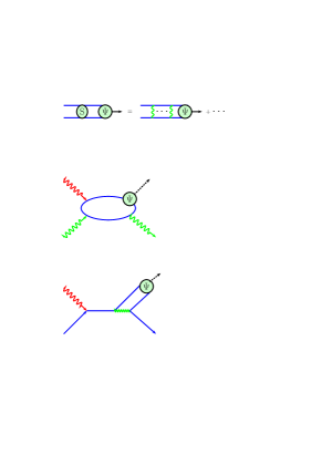
Figure 1: Typical lowest order Feynman graphs for the two subprocesses of meson electroproduction.

As is well-known from extensive studies of electromagnetic form factors at large momentum transfer leading-twist calculations are instable in the end-point regions since contributions from large transverse separations, ${\bf b}$, of quark and antiquark forming the meson are not sufficiently suppressed. In oder to eliminate that defect the so-called modified perturbative approach has been invented [7] in which the quark transverse degrees of freedom are retained and the accompanying gluon radiation is taken into account. Thus, for the quarks and antiquarks entering the meson one allows for quark transverse momenta, ${\bf k}_{\perp}$, with respect to the meson’s momentum. In addition, as suggested in Ref. [14], one also makes allowance for a meson light-cone wavefunction $\Psi_{V}(\tau,k_{\perp})$ where $\tau$ is the fraction of the light-cone plus component of the meson’s momentum the quark carries; the antiquark carries the fraction $\bar{\tau}\,=\,1-\tau$. In Ref. [7] the gluon radiation has been calculated in the next-to-leading-log (NLL) approximation using resummation techniques and having recourse to the renormalization group. The quark-antiquark separation ${\bf b}$ in configuration space acts as an infrared cut-off parameter. Radiative gluons with wave lengths between the infrared cut-off and an upper limit (related to the hard scale $Q^{2}$) yield suppression, softer gluons are part of the meson wavefunction while harder ones are an explicit part of the subprocess amplitude. Congruously, the factorization scale is given by the quark-antiquark separation, $\mu_{F}=1/b$, in the modified perturbative approach. In axial gauge the Sudakov factor can be regarded as a modification of the meson’s wavefunction [7] in a fashion that is depicted in Fig. 2.

Here in this work we are going to employ the modified perturbative approach too. In contrast to Ref. [4] we still consider the partons entering the subprocess as being emitted and reabsorbed by the proton collinearly. This supposition relies on the fact that all Fock states of the proton contribute to the GPDs. Hence, the r.m.s. ${\bf k}_{\perp}$ of the partons inside the proton reflects the charge radius of the proton (i.e. $\langle{\bf k}_{\perp}^{2}\rangle^{1/2}\simeq 200\,\,{\rm MeV}$). Only a mild ${\bf k}_{\perp}$ dependence of the GPDs is therefore to be expected. This is to be contrasted with the situation for the meson where the hard process only feeds its valence Fock state. The compactness of the latter entails much larger values of ${\bf k}_{\perp}$. The modified perturbative approach applied to the subprocess, is to some extent similar to the mechanism proposed in Ref. [15] for the suppression of the gluon contribution to meson electroproduction in the leading $\ln(1/x_{\rm Bj})$ approximation [5].

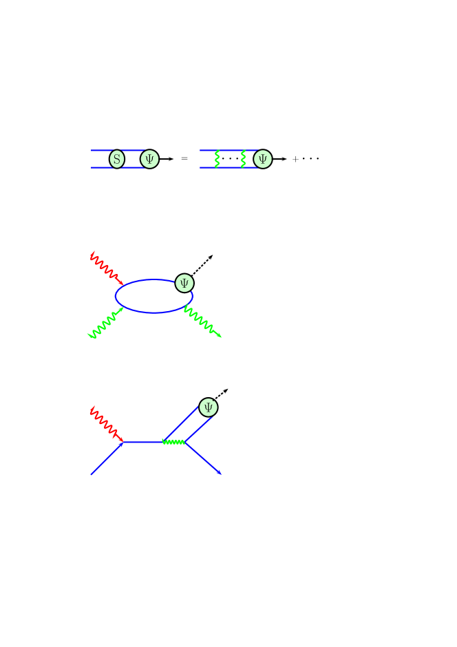
Figure 2: Illustration of gluonic radiative corrections in axial gauge.

Since the resummation of the logs involved in the Sudakov factor can only efficiently be performed in the impact parameter space [7] we have to Fourier transform the lowest-order subprocess amplitudes to that space and to multiply them there with the Sudakov factor. This leads to ($i=g,q$)

$${\cal H}_{V}^{i}\,=\,\int d\tau d^{2}b\,\hat{\Psi}_{V}(\tau,-{\bf b})\,\hat{\cal F}_{V}^{i}(\bar{x},\xi,\tau,Q^{2},{\bf b})\,\alpha_{s}(\mu_{R})\,{\rm exp}{[-S(\tau,{\bf b},Q^{2})]}\,.$$ (10)

The two-dimensional Fourier transformation between the canonical conjugated ${\bf b}$ and ${\bf k}_{\perp}$ spaces is defined by

$$\hat{f}({\bf b})\,=\,\frac{1}{(2\pi)^{2}}\int d^{\,2}\,{\bf k}_{\perp}\,\exp{[-i\,{\bf k}_{\perp}\cdot{\bf b}\,]}\;f({\bf k}_{\perp})\,.$$ (11)

The Sudakov exponent $S$ in (10) is given by [7]

$$S(\tau,b,Q)=s(\tau,b,Q)+s(\bar{\tau},b,Q)-\frac{4}{\beta_{0}}\ln\frac{\ln\left(\mu_{R}/\Lambda_{QCD}\right)}{\hat{b}}\,,$$ (12)

where a Sudakov function $s$ occurs for each quark line entering the meson and the abbreviation

$$\hat{b}\,=\,-\ln{\left(b\Lambda_{\rm{QCD}}\right)}\,,$$ (13)

is used. The last term in (12) arises from the application of the renormalization group equation ($\beta_{0}=11-\frac{2}{3}n_{f}$) where $n_{f}$ is the number of active flavors. A value of $220\,\,{\rm MeV}$ for $\Lambda_{QCD}$ is used here and in the evaluation of $\alpha_{s}$ from the one-loop expression. The renormalization scale $\mu_{R}$ is taken to be the largest mass scale appearing in the hard scattering amplitude, i.e. $\mu_{R}=\max\left(\tau Q,\bar{\tau}Q,1/b\right)$. This choice avoids large logs from higher orders pQCD. Since the bulk of the handbag contribution to the amplitudes is accumulated in regions where $\mu_{R}$ is smaller than $3\,\,{\rm GeV}$ we have to deal with three active flavors, i.e. we take $n_{f}=3$. For small $b$ there is no suppression from the Sudakov factor; as $b$ increases the Sudakov factor decreases, reaching zero at $b=1/\Lambda_{QCD}$. For even larger $b$ the Sudakov is set to zero . The Sudakov function $s$ reads

$$s(\tau,b,Q)=\frac{8}{3\beta_{0}}\left(\hat{q}\ln{\left(\frac{\hat{q}}{\hat{b}}\right)}-\hat{q}+\hat{b}\right)+{\rm NLL-terms}\,,$$ (14)

where

$$\hat{q}\,=\,\ln{\left(\tau Q/(\sqrt{2}\Lambda_{\rm{QCD}})\right)}\,.$$ (15)

Actually we do not use the version of the NLL terms quoted in Ref. [7] but rather that one given in Ref. [16]. The latter one includes some minor corrections which are hardly relevant numerically. Due to the properties of the Sudakov factor any contribution to the amplitudes is damped asymptotically, i.e. for $\ln(Q^{2}/\Lambda_{\rm{QCD}}^{2})\to\infty$, except those from configurations with small quark-antiquark separations.

The hard scattering kernels ${\cal F}_{V}^{i}$ or their Fourier transform $\hat{{\cal F}}_{V}^{i}$ occurring in Eq. (10) are computed from the pertinent Feynman graphs, see Fig. 1. The result for the gluon subprocess is discussed in some detail in Ref. [1] and we refrain from repeating the lengthy expressions here. For quarks, on the other hand, the hard scattering kernel reads

$${\cal F}_{V}^{q}\,=\,C_{F}\sqrt{\frac{2}{N_{c}}}\,\frac{Q}{\xi}\,\left[\frac{1}{k_{\perp}^{2}+\bar{\tau}(\bar{x}+\xi)Q^{2}/(2\xi)-i\epsilon}-\frac{1}{k_{\perp}^{2}-\tau(\bar{x}-\xi)Q^{2}/(2\xi)-i\epsilon}\right]\,,$$ (16)

where $N_{c}$ denotes the number of colors and $C_{F}=(N_{c}^{2}-1)/(2N_{c})$ is the usual color factor. Here and in the gluon kernel as well we only retain $k_{\perp}$ in the denominators of the parton propagators where it plays a crucial role. Its square competes with terms $\propto\tau(\bar{\tau})Q^{2}$ which become small in the end-point regions where either $\tau$ or $\bar{\tau}$ tends to zero.

The denominators of the parton propagators in (16) and in the gluonic kernel are either of the type

$${T}_{1}\,=\,\frac{1}{{\bf k}_{\perp}^{2}+d_{1}Q^{2}}\,,$$ (17)

or

$$T_{2}\,=\,\frac{1}{{\bf k}_{\perp}^{2}-d_{2}(\bar{x}\pm\xi)Q^{2}-i\varepsilon}\,.$$ (18)

where $d_{i}\geq 0$. The Fourier transforms of these propagator terms can readily be obtained:

$$\hat{T}_{1} = \frac{1}{2\pi}\,K_{0}(\sqrt{d_{1}}\,bQ)\,,$$

$$\hat{T}_{2} = \frac{1}{2\pi}\,K_{0}\left(\sqrt{d_{2}(\pm\xi-\bar{x})}\,bQ\right)\;\theta(\pm\xi-\bar{x})$$ (19)

$$+ \frac{i}{4}\,H^{(1)}_{0}\left(\,\sqrt{d_{2}\,(\,\bar{x}\pm\xi\,)}\,bQ\right)\;\theta(\,\bar{x}\pm\xi\,)\,,$$

where $K_{0}$ and $H_{0}^{(1)}$ are the zeroth order modified Bessel function of second kind and Hankel function, respectively.

For the purpose of comparison we also quote the leading-twist results (i.e. the limit $k_{\perp}\to 0$) for the subprocess amplitudes

$${\cal H}_{V({\rm l.t.})}^{g} = \frac{8\pi\alpha_{s}}{N_{c}Q}f_{V}\langle 1/\tau\rangle_{V}\,\Big{[}(\bar{x}-\xi)(\bar{x}-\xi+i\varepsilon)\Big{]}^{-1}\,,$$

$${\cal H}_{V({\rm l.t.})}^{q} = \frac{4\pi\alpha_{s}}{N_{c}Q}f_{V}\langle 1/\tau\rangle_{V}\,C_{F}\,\Big{[}\frac{1}{\bar{x}-\xi+i\epsilon}+\frac{1}{\bar{x}+\xi-i\epsilon}\Big{]}\,.$$ (20)

Here the $f_{V}$ denote the decay constants of the vector mesons for which we adopt the values $f_{\rho}\,=\,209\,\,{\rm MeV}$, $f_{\phi}\,=\,221\,\,{\rm MeV}$ and $f_{\omega}\,=\,187\,\,{\rm MeV}$ from Ref. [17]. The $1/\tau$ moment of the meson’s distribution amplitude which represents its wavefunction integrated over $k_{\perp}$ (up to the factorization scale), is denoted by $\langle 1/\tau\rangle_{V}$. In deriving Eq. (20) use is made of the fact that the distribution amplitudes for the vector mesons we are interested in are symmetric under the exchange $\tau\leftrightarrow\bar{\tau}$.

3 Modeling the GPDs

As in Ref. [1] we construct the GPDs with the help of the double distributions invented by Radyushkin [8]. The main advantage of this construction is the warranted polynomiality of the resulting GPDs and the correct forward limit $\xi,t\to 0$. It is well-known that at low $x$ the parton distribution functions (PDFs) behave as powers $\delta_{i}$ of $x$. These powers are assumed to be generated by Regge poles [18] and for sea and valence quarks they are identified with the ususal Regge intercepts $\alpha_{i}(0)$. As a consequence of the familiar definition of the gluon GPD which reduces to $xg(x)$ in the forward limit, the power $\delta_{g}$ is shifted by -1 as againts the intercept of the corresponding Regge trajectory. We generalize this behavior of the PDFs by assuming that the $t^{\prime}$ dependence of the GPDs is also under control of Regge behavior (for a similar ansatz see Ref. [19]). In order to simplify matters we consider only two trajectories: a gluon one, $\alpha_{g}(t^{\prime})$, which is understood as the hard physics partner of the famous Pomeron trajectory playing a prominent role in soft high energy diffractive scattering, and a Regge trajectory for the valence quarks, $\alpha_{\rm val}(t^{\prime})$. This trajectory represents the family of the leading Regge poles that couple to the valence quarks of the proton ($\rho$, $\omega$, $a_{2}$ and $f_{2}$ exchange in soft scattering). Since the sea quarks mix with the gluons under evolution it seems plausible to use the gluon trajectory for the sea quark GPDs as well. This assumption is supported to some extent by the observation that the ratios of the various sea quark PDFs over the gluon one are approximately independent of $Q^{2}$ at low $x$ and for $Q^{2}\raisebox{-4.0pt}{$\,\stackrel{{\scriptstyle\textstyle>}}{{\sim}}\,$}4\,\,{\rm GeV}^{2}$. The trajectories are assumed to be linear functions of $t^{\prime}$ in the small-$t^{\prime}$ range

$$\alpha_{i}\,=\,\alpha_{i}(0)+\alpha^{\prime}_{i}t^{\prime}\,,\qquad\qquad i=g,{\rm val}\,,$$ (21)

and are accompanied by Regge residues assumed to have an exponential $t^{\prime}$ dependence with slope parameters $b_{i}$.

Following Radyushkin [8] but generalizing to non-zero $t^{\prime}$, we employ the following ansatz for the double distributions ($i=g$, sea, val)

$$f_{i}(\beta,\alpha,t^{\prime})\,=\,{\rm e}^{(b_{i}+\alpha_{i}^{\prime}\ln(1/|\beta|))t^{\prime}}\,h_{i}(\beta)\,\frac{\Gamma(2n_{i}+2)}{2^{2n_{i}+1}\,\Gamma^{2}(n_{i}+1)}\,\frac{[(1-|\beta|)^{2}-\alpha^{2}]^{n_{i}}}{(1-|\beta|)^{2n_{i}+1}}\,,$$ (22)

where

$$h_{g}(\beta)\; = |\beta|g(|\beta|)\,\hskip 66.78049ptn_{g}\;=2\,,$$

$$h^{q}_{\rm sea}(\beta) = q_{\rm sea}(|\beta|)\;{\rm sign}(\beta)\hskip 30.35657ptn_{\rm sea}=2\,,$$

$$h^{q}_{\rm val}(\beta) = q_{\rm val}(\beta)\,\Theta(\beta)\hskip 50.73544ptn_{\rm val}=1\,.$$ (23)

For the decomposition of the double distribution into valence and sea contribution we follow the procedure proposed in Ref. [9] (for earlier discussions on this decomposition see [4, 20]) and write

$$f^{q}_{\rm val}(\beta,\alpha,t^{\prime}) = \big{[}f^{q}(\beta,\alpha,t^{\prime})+f^{q}(-\beta,\alpha,t^{\prime})\big{]}\,\Theta(\beta)\,,$$

$$f^{q}_{\rm sea}(\beta,\alpha,t^{\prime}) = f^{q}(\beta,\alpha,t^{\prime})\,\Theta(\beta)\,-\,f^{q}(-\beta,\alpha,t^{\prime})\,\Theta(-\beta)\,.$$ (24)

In the forward limit ($\xi,t^{\prime}\to 0$) this decomposition is conform to the usual definition of sea and valence quark PDFs.

According to Ref. [8] the GPDs are related to the double distributions by the integral

$$H_{i}(\bar{x},\xi,t^{\prime})\,=\,\int_{-1}^{1}d\beta\,\int_{-1+|\beta|}^{1-|\beta|}d\alpha\,\delta(\beta+\xi\alpha-\bar{x})\,f_{i}(\beta,\alpha,t^{\prime})\,.$$ (25)

For convenience we employ an expansion of the PDFs 

$$h_{i}(\beta)\,=\,\beta^{-\delta_{i}}\,(1-\beta)^{\,2n_{i}+1}\;\sum_{j=0}^{3}\,c_{ij}\,\beta^{j/2}\,,$$ (26)

which is particularly useful at low $\beta$ and allows to perform the integral (25) term by term analytically. This results in a corresponding expansion of the GPDs

$$H_{i}(\bar{x},\xi,t^{\prime})\,=\,{\rm e}^{b_{i}t^{\prime}}\,\sum_{j=0}^{3}\,c_{ij}\,H_{ij}(\bar{x},\xi,t^{\prime})\,.$$ (27)

For gluons and sea quarks  the individual terms read ($\epsilon_{g}=1$, $\epsilon_{\rm sea}=-1$, $m_{gj}=3+j/2-\delta_{g}-\alpha_{g}^{\prime}t$, $m_{{\rm sea}\,j}=m_{gj}-1$) [8]

$$H_{ij}(\bar{x},\xi,t^{\prime}) = \frac{15}{2\xi^{5}}\,\frac{\Gamma(m_{ij}-2)}{\Gamma(m_{ij}+3)}\,\left\{\left[(m_{ij}^{2}+2)(\xi^{2}-\bar{x})^{2}-(m_{ij}^{2}-1)(1-\xi^{2})(\bar{x}^{2}-\xi^{2})\right]\right.$$ (28)

$$\times \left.\left[x_{1}^{m_{ij}}-x_{2}^{m_{ij}}\right]+3m_{ij}\,\xi(1-\bar{x})(\xi^{2}-\bar{x})\left[x_{1}^{m_{ij}}+x_{2}^{m_{ij}}\right]\right\}\qquad\bar{x}\geq\xi$$

$$= \frac{15}{2\xi^{5}}\,\frac{\Gamma(m_{ij}-2)}{\Gamma(m_{ij}+3)}\,\left\{x_{1}^{m_{ij}}\left[(m_{ij}^{2}+2)(\xi^{2}-\bar{x})^{2}+3m_{ij}\,\xi(\xi^{2}-\bar{x})(1-\bar{x})\right.\right.$$

$$\left.\left.-(m_{ij}^{2}-1)(1-\xi^{2})(\bar{x}^{2}-\xi^{2})\right]+\epsilon_{i}(\bar{x}\to-\bar{x})\right\}\qquad 0\leq\bar{x}<\xi\,,$$

and for valence quarks ($m_{{\rm val}\,j}=2+j/2-\delta_{\rm val}-\alpha^{\prime}_{\rm val}t$)

$$H_{{\rm val}\,j}(\bar{x},\xi,t^{\prime}) = \frac{3}{2\xi^{3}}\,\frac{\Gamma(m_{{\rm val}\,j}-1)}{\Gamma(m_{{\rm val}\,j}+2)}\,$$ (29)

$$\times \left\{(\xi^{2}-\bar{x})(x_{1}^{m_{{\rm val}\,j}}-x_{2}^{m_{{\rm val}\,j}})+m_{{\rm val}\,j}\,\xi(1-\bar{x})(x_{1}^{m_{{\rm val}\,j}}+x_{2}^{m_{{\rm val}\,j}})\right\}\quad\,\bar{x}\geq\xi$$

$$= \frac{3}{2\xi^{3}}\,\frac{\Gamma(m_{{\rm val}\,j}-1)}{\Gamma(m_{{\rm val}\,j}+2)}\,x_{1}^{m_{{\rm val}\,j}}\left[\xi^{2}-\bar{x}+m_{{\rm val}\,j}\,\xi(1-\bar{x})\right]\quad-\xi\leq\bar{x}<\xi\,.$$

In Eqs. (29) and (28) we use the short-hand expressions

$$x_{1}\,=\,\frac{\bar{x}+\xi}{1+\xi}\,,\qquad x_{2}\,=\,\frac{\bar{x}-\xi}{1-\xi}\,,\qquad x_{3}\,=\,\frac{\bar{x}-\xi}{1+\xi}\,.$$ (30)

The definition of the GPDs is completed by the relations

$$H^{g}(-\bar{x},\xi,t^{\prime})\,=\,H^{g}(\bar{x},\xi,t^{\prime})\,,\qquad H_{\rm sea}^{q}(-\bar{x},\xi,t^{\prime})\,=\,-H_{\rm sea}^{q}(\bar{x},\xi,t^{\prime})\,,$$ (31)

and

$$H_{\rm val}^{q}(\bar{x},\xi,t^{\prime})\,=\,0\,\hskip 43.36464pt-1\geq\bar{x}<-\xi\,.$$ (32)

The GPDs and their derivatives up to order $n_{i}$ are continuous at $\bar{x}\,=\,\xi$. In the present work we do not consider the full evolution of the GPDs. We rather approximate it by that of the PDFs. Since for $\xi\ll\bar{x}$ and $t^{\prime}\simeq 0$ the GPDs turn into the corresponding PDFs up to corrections of order $\xi^{2}$, evolution is therefore taken into account in that region approximately. The corrections to the PDFs are of different size - they are very small for the gluon and largest for the sea quarks. The approximative treatment of evolution receives further support by the fact that at low skewness the dominant contribution to the longitudinal cross section is provided by the imaginary part of the amplitude (3). The imaginary part is related to the GPDs at $\bar{x}\simeq\xi$ (here differences between $\bar{x}$ and $\xi$ are of order $\langle k^{2}_{\perp}\rangle/Q^{2}$) which read for $\xi\ll 1$:

$$H^{g}(\xi,\xi,t^{\prime}) = \frac{2\xi g(2\xi)\;{\rm e}^{(b_{g}+\alpha_{g}^{\prime}\ln{[(1+\xi)/(2\xi)]})t^{\prime}}}{(1-\delta_{g}/5-\alpha_{g}^{\prime}t^{\prime}/5)(1-\delta_{g}/4-\alpha_{g}^{\prime}t^{\prime}/4)(1-\delta_{g}/3-\alpha_{g}^{\prime}t^{\prime}/3)}\,,$$

$$H^{q}_{\rm val}(\xi,\xi,t^{\prime}) = \frac{q_{\rm val}(2\xi)\;{\rm e}^{(b_{{\rm val}}+\alpha_{\rm val}^{\prime}\ln{[(1+\xi)/(2\xi)]})t^{\prime}}}{(1-\delta_{\rm val}/3-\alpha_{\rm val}^{\prime}t^{\prime}/3)(1-\delta_{\rm val}/2-\alpha_{\rm val}^{\prime}t^{\prime}/2)}\,.$$ (33)

For sea quarks one has to replace $\delta_{g}$ by $\delta_{\rm sea}=1+\delta_{g}$ in the first equation. Hence, at least at small $\xi$, evolution of the GPDs is approximately taken into account. The implementation of the full evolution is left to a forthcoming paper. From Eq. (33) one may also read off the so-called skewing effect [20, 21, 22], i.e. the enhancement of the GPDs at $\bar{x}=\xi$ and at $t^{\prime}=0$ over the corresponding PDFs taken at the momentum fraction $2\xi$. For the gluons the skewing effect provides the difference between the leading-twist result for vector meson electroproduction and the leading-log approximation [5] for which $H^{g}(\xi,\xi,t^{\prime}\simeq 0)$ is replaced by $2\xi g(2\xi)$. It is easy to see from Eqs. (27), (28) and (33) that the leading-log approximation is only valid at very low $\xi$. One may also see from Eq. (33) that the use of the $n=1$ model for the sea quarks would lead to implausibly large values for $H_{\rm sea}(\xi,\xi,t^{\prime})$. This is another reason why we prefer the $n=2$ GPD model for the sea quarks.

In Eq. (25) so-called $D$ terms for gluons and sea quarks are ignored [23]. The $D$ terms ensure the appearance of the highest powers of the skewness in the moments of the GPDs. According to the above discussion the $D$ terms only contribute to the less important real part of the amplitude since their support is the region $-\xi\leq\bar{x}\leq\xi$. We take this in vindication of neglecting the $D$ terms.

4 Fixing the parameters

In this section we are going to fix the parameters of our model and to present numerical results for the GPDs. For the evaluation of the latter we have to choose a set of PDFs and to expand them according to Eq. (26). Let us begin with the gluon PDF. The data used in current PDF analyses, e.g. Refs. [24, 25, 26, 27, 28, 29], do not constrain the parton distributions well for $\beta\raisebox{-4.0pt}{$\,\stackrel{{\scriptstyle\textstyle<}}{{\sim}}\,$}10^{-2}$ at low $Q^{2}$ [30]. This is evident from Fig. 3 where different versions of $\beta g(\beta)$ are displayed  at the scale $4\,\,{\rm GeV}^{2}$; the deviations diminish with increasing scale.

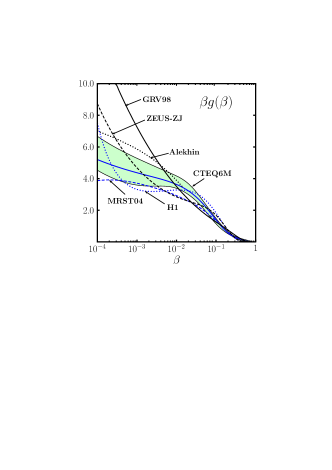
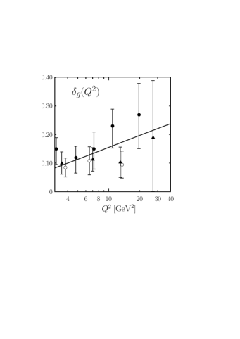
Figure 3: Left: Current gluon PDFs versus $\beta$ at a scale of $4\,\,{\rm GeV}^{2}$ [24, 25, 26, 27, 28, 29]. For the CTEQ6M solution only the band of Hessian errors is shown. Its width is typical of all PDFs. The central solid line represents the gluon PDF used in this work. Right: The intercept $\delta_{g}$ versus $Q^{2}$ at $W=75\,\,{\rm GeV}$. The fit $\delta_{g}=0.10+0.06\ln{Q^{2}/Q^{2}_{0}}$ is compared to the HERA data for $\rho$ (solid circles [11], triangles [12]) and $\phi$ electroproduction (open circles [13]).

The uncertainties in the gluon PDF matter to vector meson electroproduction. Via Eqs. (22), (25) and (5) they propagate to the cross section and lead to corresponding uncertainties there. In order to overcome this deficiency we adjust the low-$\beta$ behavior of the gluon PDF in such a way that good agreement with the HERA data on $\rho$ and $\phi$ electroproduction is achieved. Using Eqs. (4), (5) and (33), one readily obtains from the imaginary part of the gluon contribution

$$\sigma_{L}\propto W^{\,4\,\delta_{g}(Q^{2})}\,,$$ (34)

at fixed $Q^{2}$ and small $x_{\rm Bj}$; the real part does not affect the energy dependence [1]. This result allows for a determination of the intercept of the gluon trajectory. We stress that with $\delta_{\rm sea}=1+\delta_{g}$ the sea quark contribution leads to the same energy dependence of the cross section as the gluon and is in so far included in (34). For the large energy available at HERA the contributions from the valence quarks are negligible.

The power $\delta_{g}$ has been extracted from the HERA data [11, 12, 13] on the electroproduction cross section. The results are shown in Fig. 3. Since the ratio of the longitudinal and transverse cross section is only mildly energy dependent the difference between the energy dependence of the full cross section and of $\sigma_{L}$ is marginal. A straight-line fit to the HERA data is also shown in Fig. 3 and its parameters are quoted in Tab. 1. Keeping this result on $\delta_{g}$ subsequently fixed, the coefficients $c_{gj}$ in Eq. (26) are fitted to the CTEQ6M gluon PDF [24] in the range $4\,\,{\rm GeV}^{2}\leq Q^{2}\leq 40\,\,{\rm GeV}^{2}$ and $10^{-4}\leq\beta\leq 0.5$. The values obtained for the coefficients are given in Tab. 1 as well. The resulting fit is also shown in Fig. 3. In the quoted range of $Q^{2}$ and for $\beta$ the fit agrees very well with the CTEQ6M solution; it is always well inside the band of Hessian errors, see Fig. 3. Larger values of $\beta$ are irrelevant to us since the contribution of the GPDs from the region $0.5\raisebox{-4.0pt}{$\,\stackrel{{\scriptstyle\textstyle<}}{{\sim}}\,$}\beta$ to the real part of the amplitude is less than $0.5\%$. From the gluon PDF just described we evaluate the gluon GPD with the help of Eqs. (27) and (28). For a set of skewness values it is shown in Fig. 4. In the context of the error assessment to be executed below, we will comment on the implications of the other PDF solutions.

	gluon	strange	$u_{\rm val}$	$d_{\rm val}$
$\delta$	$0.10+0.06\,L$	$1+\delta_{g}$	0.48	0.48
$c_{0}$	$2.23+0.362\,L$	$\phantom{-}0.123+0.0003\,L$	$1.52+0.248\,L$	$0.76+0.248\,L$
$c_{1}$	$\phantom{-}5.43-7.00\,L$	$-0.327-0.004\,L$	$2.88-0.940\,L$	$\phantom{-}3.11-1.36\,L$
$c_{2}$	$-34.0+22.5\,L$	$\phantom{-}0.692-0.068\,L$	$-0.095\,L$	$-3.99+1.15\,L$
$c_{3}$	$\phantom{-}40.6-21.6\,L$	$-0.486+0.038\,L$	$0$	$0$

Table 1: The parameters appearing in the expansion (26) of the PDFs ($L=\ln{Q^{2}/Q^{2}_{0}}$, $Q^{2}_{0}=4\,\,{\rm GeV}^{2}$). The expansion provide fits to the CTEQ6M PDFs [24] in the range $10^{-2}\leq\beta\leq 0.5$ and $4\,\,{\rm GeV}^{2}\leq Q^{2}\leq 40\,\,{\rm GeV}^{2}$. The powers $\delta$ are kept fixed in the fits.

A power $\delta_{g}$ rising with $Q^{2}$, is untypical for the Regge-pole model. Even more important, $\delta_{g}>0$ leads to a cross section that increases as a power of the energy, see Eq. (34). At very high energies, it will therefore violate the Froissart bound and, hence, unitarity. Obviously, there must occur a saturation at some scale of $Q^{2}$ that will limit the rise of the gluon PDF and GPD and will restore unitarity. In other words, the description of diffraction by a Pomeron-type pole with an intercept, $\alpha_{g}(0)$, larger than unity is to be considered as an effective parameterization that holds in a finite although possibly large range of energy [31]. Unitarity will ultimately force the generation of a series of shielding cuts [32] that will prevent the violation of the Froissart bound. An effective parameterization may have parameters that dependent on the process and on the kinematics.

For the slope of the gluon trajectory we take the value $\alpha_{g}^{\prime}=0.15\,\,{\rm GeV}^{-2}$ which is slightly smaller than that of the usual soft Pomeron [31] but agrees with the value observed in photoproduction of the $J/\Psi$ [33] and other vector mesons [34]. Small values of the gluon and soft Pomeron slopes are required since the diffraction peaks show little shrinkage.

Using $\delta_{\rm sea}=1+\delta_{g}$ we perform an analogous fit of the strange quark CTEQ6M distribution (assuming $s(\beta)=\bar{s}(\beta)$). The parameters are quoted in Tab. 1 too and the resulting GPD $H^{s}_{\rm sea}$ constructed through the double distribution (22) is shown in Fig. 4. For the CTEQ6M PDFs [24] the $\bar{u}$ and $\bar{d}$ distributions at low $\beta$ are very close to each other and enhanced by an approximately $Q^{2}$-dependent but $\beta$-independent factor $\kappa_{s}(Q^{2})$ as compared to the strange quark PDF. In an attempt to keep the GPD model simple we therefore assume

$$H^{u}_{\rm sea}\,=\,H^{d}_{\rm sea}\,=\,\kappa_{s}\,H^{s}_{\rm sea}\,,$$ (35)

where the flavor symmetry breaking factor is parameterized as

$$\kappa_{s}\,=\,1+0.68/(1+0.52\,\ln{Q^{2}/Q^{2}_{0}})\,,$$ (36)

as obtained from a fit to the CTEQ6M PDFs. Eq. (35) is a simplification which as one may object, is unjustified given the high level of accuracy the current PDF solution have reached. However we are constructing model GPDs which implies a theoretical uncertainty of unknown strength. It seems premature in the present state of the art to transfer the full complexity of the current PDFs to the model GPDs. It is not probed by the present data on vector meson electroproduction  and would rather confuse than elucidate the physical interpretation.

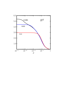
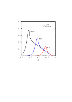
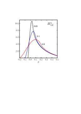
Figure 4: The GPDs $H^{g}$ (left), $H^{s}_{\rm sea}$, multiplied by $\bar{x}$, (center), and $H_{\rm val}^{u}$ (right) at selected values of skewness. The GPDs are shown at $t^{\prime}=0$ and at a scale of $4\,\,{\rm GeV}^{2}$.

For the valence trajectory we adopt standard soft physics parameters, $\alpha_{\rm val}(0)=0.48$ and $\alpha_{\rm val}^{\prime}=0.9\,\,{\rm GeV}^{-2}$. This is in fair agreement with the low-$x$ behavior of the valence quark PDFs at low factorization scale (up to at least $40\,\,{\rm GeV}^{2}$) within errors. Only a very mild, negligible effect of evolution is to be observed for these parameters. Keeping again the intercept fixed we fit the expansion (26) to the $u$ and $d$ valence quark distributions of the CTEQ6M solution and evaluate the correponding GPDs from Eqs. (27) and (29). The obtained parameters are quoted in Tab. 1 and $H^{u}_{\rm val}$ at $t^{\prime}=0$ is displayed in Fig. 4. In contrast to the sea quark GPDs where the $n=1$ model is to be rejected because of its very strong skewing effect (and because of the Pomeron-type interpretation), the skewing effect for the valence quarks is much weaker.

Now having specified the parameterization of the Regge trajectories we turn to their determination of the residues, i.e. of the slope parameters $b_{i}$. As we repeatedly mentioned vector meson electroproduction behaves diffractively, i.e. its differential cross section decrease exponentially with $t^{\prime}$. In the handbag approach this behavior is to be incorporated in the gluon GPD. Although its $t^{\prime}$ dependence appears to be more complicated than an exponential as is for instance seen from Eq. (28) or (33), this is not the case in reality. They actually behave as exponentials as can be seen from Fig. 5 where we display $H^{g}(\xi,\xi,t^{\prime})$ versus $t^{\prime}$ for selected values of $W$ and $Q^{2}$. As a consequence of the smallness of $\alpha^{\prime}_{g}$ the effective slope of the gluon GPD falls together with the Regge exponential to a very high degree of accuracy, for the sea quark GPD the situation is similar. Hence, because of the repeatedly mentioned dominance of the imaginary part of the gluon contribution at HERA kinematics the slope of the differential cross section is given by

$$B_{V}\simeq 2b_{g}+2\alpha^{\prime}_{g}\ln{\frac{1+\xi}{2\xi}}\,,$$ (37)

in our model GPDs. Insertion of Eqs. (1) and (2) translates this relation into

$$B_{V}\,=\,2b_{g}+2\alpha^{\prime}_{g}\ln{\frac{W^{2}+Q^{2}}{Q^{2}+m_{V}^{2}}}\,.$$ (38)

High-energy data for the $t^{\prime}$ dependence only exist for the unseparated cross section $d\sigma=d\sigma_{T}+\varepsilon\,d\sigma_{L}$ where $\varepsilon$ is the ratio of longitudinal to transversal polarization of the virtual photon. Ignoring possible differences between the slopes of the transverse and longitudinal cross sections (which can only emerge from the subprocess amplitudes) we fit $b_{g}$ against the HERA data for $\rho$ [11] and $\phi$ production [13]. We find that the experimental slope parameters are well described by

$$b_{g}\,=\,b_{\rm sea}\,=\,2.58\,\,{\rm GeV}^{-2}+0.25\,\,{\rm GeV}^{-2}\,\ln{\frac{m^{2}}{Q^{2}+m^{2}}}\,,$$ (39)

see Fig. 5. It is to be stressed that the term $\propto\alpha_{g}^{\prime}$ in Eq. (38) is a consequence of the Regge behavior while the log term in Eq. (39) is an ansatz. The $\rho$ and $\phi$ slopes practically fall together at HERA energies; there are only minor differences at low $Q^{2}$ which are not shown in Fig. 5.

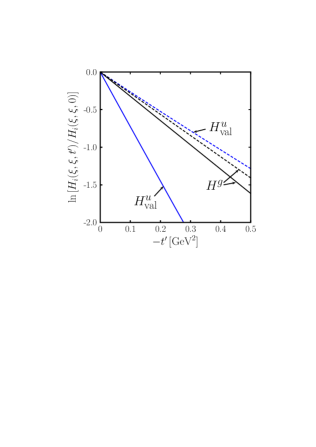
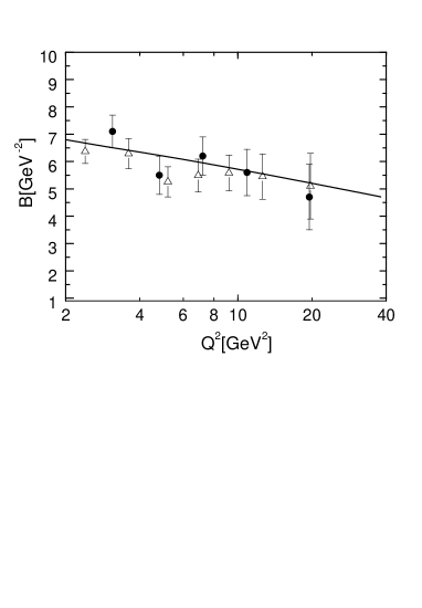
Figure 5: Left: The $t^{\prime}$ dependence of the gluon and the $u$-valence GPDs at $W=75\,\,{\rm GeV},\;Q^{2}=4\,\,{\rm GeV}^{2}$ (solid lines) and $W=5\,\,{\rm GeV}\,\;Q^{2}=3\,\,{\rm GeV}^{2}$ (dashed lines). Right: The slope $B_{V}$ of the differential cross section for $\rho$ and $\phi$ electroproduction versus $Q^{2}$ at $W=75\,\,{\rm GeV}$. Data are taken from Ref. [11] (solid circles) and [13] (open triangles). The solid line represents the fit (38), (39) for the case of the $\phi$.

The zero-skewness limit of the valence quark GPDs reads

$$H^{q}_{\rm val}(\bar{x},\xi=0,t^{\prime})\,=\,{\rm e}^{(b_{\rm val}+\alpha^{\prime}_{\rm val}\,\ln(1/\bar{x}))\,t^{\prime}}\,q_{\rm val}(\bar{x})\,,$$ (40)

as readily follows from (22) and (25). This is very close to an ansatz advocated for in Ref. [35] in order to extract the zero-skewness GPDs from the nucleon form factor data (see also Ref. [36]). Our Regge exponential appears as the small $\bar{x}$ approximation of the exponential exploited in Ref. [35]. In the range $0\raisebox{-4.0pt}{$\,\stackrel{{\scriptstyle\textstyle<}}{{\sim}}\,$}\bar{x}\raisebox{-4.0pt}{$\,\stackrel{{\scriptstyle\textstyle<}}{{\sim}}\,$}0.15$ the difference between both the exponentials is less than $10\%$. The comparison with the zero-skewness analysis further reveals that the slope of the Regge trajectory suffices to specify the $t^{\prime}$ dependence of the valence quark GPDs. Consequently we set $b_{\rm val}$ equal to zero. It is also checked by us that the valence quark GPDs (27), (29) respect the sum rule for the Dirac form factor at any value of skewness; small deviations between the form factor data and the sum rules evaluated from our GPDs occur at larger $t^{\prime}$ and amount to about $3\%$ at $t=-0.6\,\,{\rm GeV}^{2}$.

Effectively the valence quarks GPDs behave as exponentials in $t^{\prime}$ too, see Fig. 5. The decisive difference is however that the valence quark GPDs show strong shrinkage due to the large value of $\alpha^{\prime}_{\rm val}$. While at HERMES kinematics the effective slopes of the gluon and the valence quark GPDs are similar, is the latter much larger at HERA kinematics.

Last not least we have to specify the meson wavefunction occurring in Eq. (10). As in our previous work [1] and in other applications of the modified perturbative approach, e.g. [14, 16], we use a Gaussian wavefunction

$$\Psi_{V}(\tau,{\bf k}_{\perp})\,=\,8\pi^{2}\sqrt{2N_{c}}f_{V}a_{V}^{2}{\rm exp}{[-a_{V}^{2}{\bf k}_{\perp}^{2}/(\tau\bar{\tau})]}\,.$$ (41)

Transverse momentum integration of it leads to the associated distribution amplitude which represents the soft hadronic matrix element entering calculations in the collinear factorization approach. Actually, the wavefunction (41) leads to the so-called asymptotic form of the meson distribution amplitude

$$\Phi_{\rm AS}\,=\,6\tau\bar{\tau}\,.$$ (42)

Its $1/\tau$ moment occurs in the leading-twist result (20) and acquires the value 3. The transverse size parameter $a_{V}$ is considered as a free parameter fitted to the data on the integrated cross sections $\sigma_{L}$ for $\rho$ and $\phi$ production, see next section. It can be varied within a certain range of values determined by the requirement that the corresponding r.m.s. ${\bf k}_{\perp}$ being related to the transverse size parameter by

$$\langle k_{\perp}^{2}\rangle^{1/2}\,=\,\big{[}\sqrt{10}\,a_{V}\big{]}^{-1}\,,$$ (43)

acquires a plausible value consistent with our assumption of taking into account only the transverse momenta of the quarks forming the meson. A possible evolution of the transverse size parameter is ignored.

5 Results for the longitudinal cross sections

The full amplitudes for vector meson electroproduction (5), (6) are a coherent superposition of contributions from the various quark flavors and from the gluon. In order to shed light on the relative importance of the various terms we quote the leading-twist result

$${\cal M}_{\phi} = e\frac{8\pi\alpha_{s}}{N_{c}Q}\,f_{\phi}\langle 1/\tau\rangle_{\phi}\,\frac{-1}{3}\,\left\{\frac{1}{2\xi}I_{g}+C_{F}\,I_{\rm sea}\right\}\,,$$

$${\cal M}_{\rho} = e\frac{8\pi\alpha_{s}}{N_{c}Q}\,f_{\rho}\langle 1/\tau\rangle_{\rho}\,\frac{1}{\sqrt{2}}\,\left\{\frac{1}{2\xi}I_{g}+\kappa_{s}\,C_{F}\,I_{\rm sea}+\frac{1}{3}\,C_{F}\,I^{u}_{\rm val}+\frac{1}{6}\,C_{F}\,I^{d}_{\rm val}\right\}\,,$$

$${\cal M}_{\omega} = e\frac{8\pi\alpha_{s}}{N_{c}Q}\,f_{\omega}\langle 1/\tau\rangle_{\omega}\,\frac{1}{3\sqrt{2}}\,\left\{\frac{1}{2\xi}I_{g}+\kappa_{s}\,C_{F}\,I_{\rm sea}+C_{F}\,I^{u}_{\rm val}-\frac{1}{2}\,C_{F}\,I^{d}_{\rm val}\right\}\,.$$ (44)

The integrals in Eq. (44) read

$$I_{g} = 2\int_{0}^{1}d\bar{x}\frac{\xi H^{g}(\bar{x},\xi,t^{\prime})}{(\bar{x}+\xi)(\bar{x}-\xi+i\epsilon)}\,,$$

$$I_{\rm sea} = 2\int_{0}^{1}d\bar{x}\frac{\bar{x}H^{s}_{\rm sea}(\bar{x},\xi,t^{\prime})}{(\bar{x}+\xi)(\bar{x}-\xi+i\epsilon)}\,,$$

$$I^{a}_{\rm val} = 2\int_{-\xi}^{1}d\bar{x}\frac{\bar{x}H^{a}_{\rm val}(\bar{x},\xi,t^{\prime})}{(\bar{x}+\xi)(\bar{x}-\xi+i\epsilon)}\,.$$ (45)

The imaginary parts of these integrals are just $-\pi H_{i}(\xi,\xi,t^{\prime})$ and for $\xi\to 0$ they exhibit typical Regge phases as a consequence of the analytic structure of the integrals and the symmetries of the GPDs (31).

Within the modified perturbative approach the amplitudes have the same structure as in Eq. (44). Only the integrals (45) are much more complex, they do not factorize into products of integrals over the wave functions and such over the product of GPDs and propagators. Despite this the suppressions induced by the modified perturbative approach do not change much the relative strengths of the various contributions. One may therefore get an quick insight into the relative strength of the various terms from Eq. (44).

Figure 6: Real over imaginary part of the full amplitude for $\rho$ production versus $W$ at $Q^{2}=4\,\,{\rm GeV}^{2}$ and $t^{\prime}=0$.

Numerical evaluation of the amplitudes (5) and (6) reveals that, for skewness less than about 0.01, the gluon and sea contributions are dominantly imaginary while, for $\xi\simeq 0.1$, their real parts are nearly as large as their imaginary part. The valence quark contribution behaves oppositely. The energy dependence of ratio of the real and imaginary parts of the full $\rho$ production amplitude is shown in Fig. 6 at $Q^{2}=4\,\,{\rm GeV}^{2}$. A remark concerning the values of $\alpha_{s}$ is in order. As an inspection of our handbag amplitude reveals almost the entire contribution is accumulated in a comparatively narrow region of $\alpha_{s}$. For instance, at $Q^{2}=4\,\,{\rm GeV}^{2}$ and $W=5\,\,{\rm GeV}$ $90\%$ of the amplitude comes from the range $0.3\raisebox{-4.0pt}{$\,\stackrel{{\scriptstyle\textstyle<}}{{\sim}}\,$}\alpha_{s}\raisebox{-4.0pt}{$\,\stackrel{{\scriptstyle\textstyle<}}{{\sim}}\,$}0.5$ with a mean value of about 0.4. Hence, our handbag approach is theoretically self-consistent in so far as contributions from soft regions where $\alpha_{s}$ is larger than, say, 0.6 and where perturbation theory breaks down, are strongly suppressed.

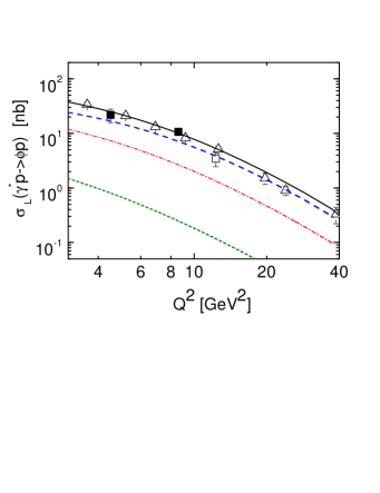
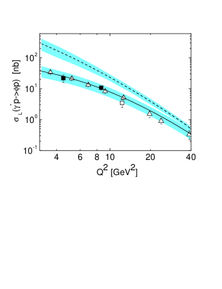
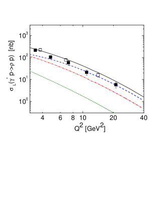
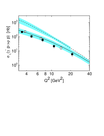
Figure 7: The longitudinal cross section for $\phi$ production at $W=75\,\,{\rm GeV}$. Data are taken from [13] (open triangles), [37] (solid squares) and [38] (open squares). Left: Full (dashed, dash-dotted, dotted) line represents the handbag predictions for the cross section (gluon, gluon-sea interference, sea contribution). Right: Predictions for the cross section with error bands resulting from the Hessian errors of the CTEQ parton distributions (full line) and compared to the leading-twist result (dashed line).

Figure 8: The longitudinal cross section for $\rho$ production at $W=75\,\,{\rm GeV}$. Data are taken from [11, 39] (solid squares) and [12] (open squares). For other notations cf. Fig. 8.

We are now ready to present our results for vector meson electroproduction. They are obtained by adjusting the transverse size parameters $a_{V}$ appropriately. The best fits provide the values

$$a_{\phi}\,=\,0.70\,\,{\rm GeV}^{-1}\,,\qquad\qquad a_{\rho}\,=\,0.75\,\,{\rm GeV}^{-1}\,.$$ (46)

The corresponding r.m.s. ${\bf k}_{\perp}$ is about $500\,\,{\rm MeV}$. This value is more than a factor of 2 larger than the corresponding value for the quarks inside the proton and is in so far consistent with our assumption of taking into account only the transverse momenta of the quarks forming the meson. In Figs. 8 and 8 we compare our results for $\phi$ and $\rho$ production to the HERA data  [11, 12, 13, 37, 38, 39]. In the left panels of these figures we show the decomposition of the cross sections into the various contributions from the gluon and the quarks. The gluon contribution is dominant but the corrections from the gluon-sea interference amount to about $25\,(50)\%$ for $\phi$ ($\rho$) production; the valence quark contribution (including its interference with the gluon and the sea) to the $\rho$ production cross section is tiny and can be neglected. The larger sea quark contribution for $\rho$ production follows from the flavor symmetry breaking factor $\kappa_{s}$. In the right panels of Figs. 8 and 8 we display in addition to our full results their uncertainties due to the Hessian errors of the CTEQ6 PDFs and for comparison the leading-twist result evaluated from the asymptotic distribution amplitude (42). Results for the cross sections evaluated from sets of PDFs other than CTEQ6 also fall into the error bands in most cases (an exception is set for instance by the PDFs determined in Ref. [29]) provided these PDFs are treated in analogy to the CTEQ6M set, i.e. they are fitted to the expansion (26) by forcing them to behave Regge-like with powers $\delta_{i}$ as described above, and if necessary readjusting the transverse size parameters. Straight-forward evaluation of the GPDs from the various sets of PDFs and fixed transverse-size parameters lead to cross sections which differ markedly stronger than the error bands indicate. For examples see Ref. [6]. The results obtained with the modified perturbative approach are in remarkable agreement with the HERA data while the leading-twist results are clearly in excess to experiment with a tendency however of approaching the data and the predictions from the modified perturbative approach at $Q^{2}\simeq 40\,\,{\rm GeV}^{2}$. This in turn tells us that the effect of the transverse quark degrees of freedom in combination with the Sudakov suppressions become small for such values of $Q^{2}$ while being very important at lower $Q^{2}$. Pertinent observations have also been made by Ivanov et al. [40]. In their next-to-leading order leading-twist calculation of vector meson electroproduction large perturbative logs occur which partly cancel the leading-order term bringing the leading-twist result closer to experiment. These logs are included in the Sudakov factor (14).

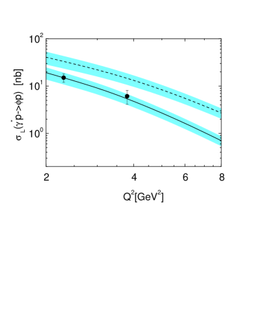
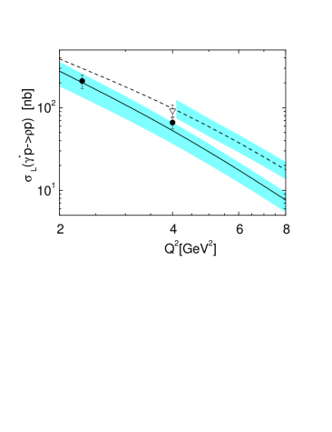
Figure 9: The longitudinal cross section for $\phi$ (left) and $\rho$ (right) production versus $Q^{2}$ at $W=5$ (solid line) and $10\,\,{\rm GeV}$ (dashed line). Data at $W=5\,\,{\rm GeV}$, shown as solid circles, are taken from HERMES [41] (for $\phi$, preliminary) and [42] (for $\rho$). The open triangle presents the E665 [43] data point at $W=10\,\,{\rm GeV}$. For other notations cf.  Fig. 8.

In Fig. 9 we show the results for $\sigma_{L}$ at $W=5$ and $10\,\,{\rm GeV}$ and compare them to the data from HERMES [41, 42] and the FERMILAB experiment E665 [43]. Again we observe good agreement with experiment. The slopes of the differential cross section are somewhat smaller at lower energies than those at the HERA energy shown in Fig. 5. For instance at $W=5\,\,{\rm GeV}$ and $Q^{2}=4\,\,{\rm GeV}^{2}$ we obtain $5.0\,\,{\rm GeV}^{-2}$ for $\rho$ production and $4.8\,\,{\rm GeV}^{-2}$ for the case of the $\phi$. As yet the HERMES collaboration has only provided preliminary results for these slopes: $6.32\pm 0.72\,\,{\rm GeV}^{-2}$ at $Q^{2}=3.7\,\,{\rm GeV}^{2}$ for $\rho$ [44] and $4.6\pm 1.2\,\,{\rm GeV}^{-2}$ averaged over the range $0.7\leq Q^{2}\leq 5\,\,{\rm GeV}^{2}$ for $\phi$ production [45]. A slope for $\rho$ production that is considerably larger than that for $\phi$ production is difficult to get in the handbag approach. Although it seems tempting to assign such an effect to the valence quark contribution by choosing a non-zero value for $b_{\rm val}$ this is likely not the solution since it would lead to a Dirac form factor that drops too fast with $t$. An alternative possibility seems to change the $t^{\prime}$ dependence of the sea quark GPD by choosing a value for $b_{\rm sea}$ larger than that for $b_{g}$ which is theoretically not forbidden. On account of the different weights of the sea contribution in both the processes of interest this may generate a somewhat larger slope in the case of the $\rho$. In regard to the present experimental situation we leave this question unanswered for the time being. Pertinent future data may settle this issue. In order to demonstrate how close the $t^{\prime}$ dependence of the differential cross section to an exponential behavior is we show in Fig. 10 the cross section for $\rho$ production at $W=5\,\,{\rm GeV}$ and $Q^{2}=4\,\,{\rm GeV}^{2}$ as an example.

Figure 10: The differential cross section for $\rho$ production versus $t^{\prime}$ at $W=5\,\,{\rm GeV}$ and $Q^{2}=4\,\,{\rm GeV}^{2}$.

Consulting Fig. 12 one sees that also the $W$ dependence of the longitudinal cross section is correctly described within the handbag approach. Note that $\sigma_{L}$ in Figs. 8, 8, 9 and 12 (left) is obtained by integrating the differential cross section over the range of $t^{\prime}$ that is used in the various experiments. Thus, we integrate from 0 to $-0.6,-0.5,-0.4\,\,{\rm GeV}^{2}$ for HERA, COMPASS (and E665), and HERMES kinematics, respectively. For $\sigma_{L}$ in Figs. 12 and 12 (right) on the other hand we integrate up to $-0.5\,\,{\rm GeV}^{2}$ throughout but compare with actual data. The cross sections exhibit kinks at about $W=10\,\,{\rm GeV}$, rather markedly for $\phi$ production, milder in the case of the $\rho$. These kinks are related to the sharp fall off of the gluon and sea quark GPDs with increasing $\xi$ (note that $\xi\propto 1/W^{2}$ at fixed $Q^{2}$), see the gluon PDF shown in Fig. 3. The additional valence quark contribution in $\rho$ production

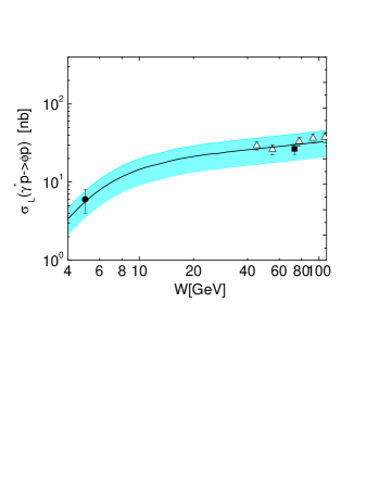
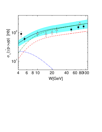
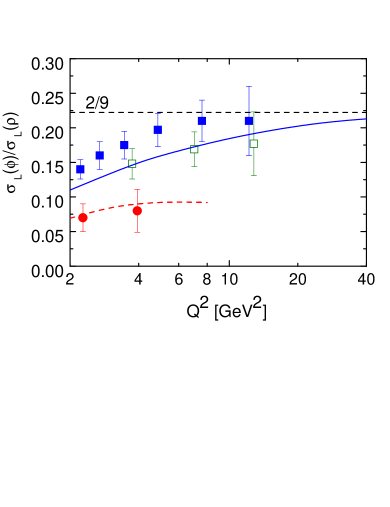
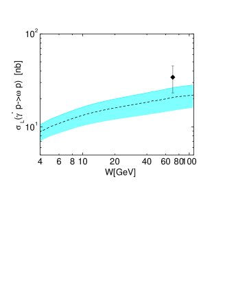
Figure 11: The longitudinal cross section for $\phi$ (left) and $\rho$ (right) electroproduction versus $W$ at $Q^{2}=3.8\,\,{\rm GeV}^{2}$ and $4\,\,{\rm GeV}^{2}$, respectively. The handbag predictions are evaluated from the interval $-t^{\prime}\leq 0.5\,\,{\rm GeV}^{2}$. Data for $\phi$ production are taken from HERMES [41] (solid circle), ZEUS [13] (open triangles) and H1 [37] (solid square). The data for $\rho$ production are taken from HERMES [42] (solid circles), E665 [43] (open triangles), ZEUS [12] (open square) and H1 [11] (solid square). The dashed (dash-dotted, dash-dot-dotted) line represents the gluon (gluon + sea, (gluon + sea)-valence interference plus valence quark) contribution. For other notations cf.  Fig. 8.

Figure 12: Left: The ratio of the longitudinal cross sections for $\phi$ and $\rho$ production. Data are taken from H1 [11, 37] (solid squares), ZEUS [12, 13] (open squares) and HERMES [41, 42] (solid circles). The solid (dashed) line represents the handbag predictions at $W=75(5)\,\,{\rm GeV}$. Right: Predictions for $\omega$ electroproduction versus $W$ at $Q^{2}=3.5\,\,{\rm GeV}^{2}$. For comparison the full cross section for $\omega$ production, measured by ZEUS [49], is also shown (solid diamond).

mitigates the kink. For $\rho$ production we also show in Fig. 12 the individual contributions from the gluons, sea and valence quarks. At $W\simeq 5\,\,{\rm GeV}$ the latter contribution (including the interference with the gluon and sea quarks) amounts to about $50\%$ of the full result but decreases rapidly with increasing $W$. It only contributes about $10\%$ at $W=10\,\,{\rm GeV}$ and is negligible at the HERA energy.

All the results we presented so far are evaluated from the Gaussian wavefunction (41). One may wonder what the consequences of other choices of the wavefunction are. In order to provide a partial answer to this question we multiply the wavefunction (41) for the $\rho$ meson with the factor

$$1+B_{2}(\mu_{0})\,\left[\frac{\alpha_{s}(\mu_{F})}{\alpha_{s}(\mu_{0})}\right]^{50/81}\,C_{2}^{3/2}(2\tau-1)\,.$$ (47)

It corresponds to the first two terms of the expansion of the meson distribution amplitude upon the Gegenbauer polynomials $C_{n}^{3/2}$, the eigenfunctions of the evolution kernel for mesons [46]. For an estimate of the impact of that factor on the cross section for $\rho$ production we adopt the value

$$B_{2}(\mu_{0}=1\,\,{\rm GeV})\,=\,0.18\,,$$ (48)

obtained from QCD sum rules for the expansion coefficient [47]. From this value of $B_{2}$ we find that the cross section for $\rho$ production increases by approximately $14\,(24)\%$ at $Q^{2}=4\,(20)\,\,{\rm GeV}^{2}$ in the entire range of energy we examine. This is well within the uncertainties of our approach which are represented by the error bands shown in the various figures. The gradual decrease of the second Gegenbauer term with increasing scale is to a large extent compensated by the diminishing suppression through the quark transverse momenta and the Sudakov factor. In a calculation to leading-twist order the effect of the higher Gegenbauer terms is more pronounced at low $Q^{2}$. For instance, at $Q^{2}=4\,\,{\rm GeV}^{2}$ the $\rho$ cross section increases by $31\%$ to leading-twist order using (48) and $\mu_{F}=Q$.

In the limit of negligible valence quark contributions one has the following relative strength of the three cross sections: $\rho\,:\,\omega\,:\,\phi=1\,:\,9\,:\,2/9$ up to flavor symmetry breaking effects as the differences in the decay constants and in the wavefunction or distribution amplitudes or the flavor symmetry breaking factor (36) in the sea GPDs. While the latter two effects disappear for $Q^{2}\to\infty$ due to evolution, the differences in the decay constants are scale independent. Hence, for very large scales the handbag approach predicts

$$\sigma_{L}(\phi)/\sigma_{L}(\rho)\Longrightarrow\frac{2}{9}\,\left(\frac{f_{\phi}}{f_{\rho}}\right)^{2}\,=\,0.248\,.$$ (49)

An analogous result holds for the ratio of the $\omega$ and $\rho$ cross sections. The HERA data [11, 12, 13, 37] shown in Fig. 12, are not far from the symmetry limit $2/9$ especially at larger values of $Q^{2}$ but the face values are clearly below it. The evolution effect of a $\rho$ wave function broader in $\tau$ than the Gaussian given in Eq. (41) is too mild if one accepts the QCD sum rule estimate of the Gegenbauer coefficients, see above discussion. It does not explain the $Q^{2}$ dependence of the data. Thus, we are compelled to conclude that the bulk of the effect seen in the HERA data is due to flavor symmetry breaking in the sea. Indeed with $\kappa_{s}$ as given in Eq. (36) we obtain the results for the ratio of the $\phi$ and $\rho$ cross sections shown in Fig. 12 which agree fairly well with experiment. The cross section ratio at the HERMES energy is smaller as at the higher HERA energy which as a glance at Eq. (44) reveals, is to be assigned to the additional valence quark contribution to the $\rho$ cross section at $W=5\,\,{\rm GeV}$ (see also Ref. [48]). Indeed our results are in agreement with the HERMES data [41, 42], see Fig. 12.

Predictions for $\omega$ production are presented in Fig. 12 as well. They are obtained by assuming $a_{\omega}=a_{\rho}$. Only the unseparated cross section has been measured by the ZEUS collaboration [49] at $W=70\,\,{\rm GeV}$ and $Q^{2}=3.5$ and therefore we cannot directly compare with our results. However, assuming that the ratio of the longitudinal and transversal cross sections is about 2 at this kinematics, one expects a longitudinal cross section that amounts to about 2/3 of the full cross section and this would be in agreement with our result. The valence quark contribution is stronger for $\omega$ than for $\rho$ production as is expected from Eq. (44). For our kinematical point of reference, $W=5\,\,{\rm GeV}$ and $Q^{2}=4\,\,{\rm GeV}^{2}$, for instance, it amounts to about $65\%$ of the $\omega$ cross section. Data on the longitudinal cross section for $\omega$ production would be highly welcome. They would provide information on a second combination of the $u$ and $d$ quark GPDs $e_{u}\,H^{u}+e_{d}\,H^{d}$.

6 Summary

We have investigated light vector-meson electroproduction within the handbag approach. The partonic subprocesses are treated within the modified perturbative approach and the GPD $H$ for gluons, sea and valence quarks is constructed from the CTEQ6M PDFs through double distributions using a Regge-inspired $t$ dependence. The GPDs $H$ respect all theoretical constraints, i.e. the reduction formulas, positivity and polynomiality as well as the sum rule for the Dirac form factor of the proton. From our approach we have obtained a fair understanding of the longitudinal cross section over a large range of energy (from $W=5$ till $100\,\,{\rm GeV}$) and photon virtualities ( from 2.5 to $40\,\,{\rm GeV}^{2}$) provided $x_{\rm Bj}$ is small. A remarkable outcome of our investigation is that the gluon contribution play an important role over the entire range of energy we have explored. The sea quarks also contribute considerably at all energies although to a lesser extent than the gluons. The valence quarks on the other hand are only of importance for $\rho$ and $\omega$ production and for energies less than about $10\,\,{\rm GeV}$.

We have simplified the parameterization of the sea quark GPDs, not all details of the PDFs are transfered to them. Thus, we have reduced the sea quark GPDs to a single function allowing for differences only through a flavor symmetry factor. At the present stage of our knowledge on the GPDs a more refined model would provide a pseudo accuracy that does not meet the uncertainties of the GPD model and that would rather confuse than elucidate. With our sea quark GPDs it becomes evident that the $Q^{2}$ dependence of the $\phi$ - $\rho$ ratio of the longitudinal cross sections at HERA energies is generated by the flavor symmetry breaking in the sea. Data for $\omega$ production may perhaps force us to improve the parameterization of the sea quark GPDs. The data for $\rho$ production alone only probe the combination $e_{u}H^{u}_{\rm sea}-e_{d}H^{d}_{\rm sea}$.

In our previous work [1] we have also calculated the amplitudes for other transitions from the virtual photon to the vector meson within the handbag approach. With them we have achieved a fair description of the transverse cross section and the spin density matrix elements at HERA energies where the gluon contribution dominates. The application of this approach to the spin density matrix elements at lower energies necessitates the inclusion of the quark contribution into the analysis which is left to a forthcoming paper.

The handbag approach with the reggeized GPDs bears similarities to other theoretical models for vector-meson electroproduction which are mainly applied to the high energy and/or very low $x_{\rm Bj}$ regime. The gluonic subprocess, see Fig. 1, with the accompanied proton-gluon vertex function forms the basis of many models. The various approaches essentially differ in the treatment of that vertex function (Pomeron residue [31, 50] or the gluon PDF in the BFKL color dipole model [34] and in the leading-log approximation [15, 21]) and in the assumptions which of the partons in the Feynman graphs are considered as soft, i.e. as quasi on-shell, and which as hard. In the handbag approach with the QCD factorization theorems [2, 3] as foundation, the protons emit and reabsorb quasi on-shell partons and the associated vertex function, a soft proton matrix element, is regarded as a GPD. The quark and antiquark entering the final state meson are also considered as on-shell particles. The associated soft $q\bar{q}\to V$ transition is parameterized as a light-cone wavefunction or distribution amplitude. All other partons in the graphs shown in Fig. 1 are highly virtual. The advantage of the handbag approach is that once the GPDs are fixed other hard exclusive processes, as for instance deeply virtual Compton scattering, can be predicted.

References

- [1] S. V. Goloskokov and P. Kroll, Eur. Phys. J. C 42, 281 (2005) [hep-ph/0501242].
- [2] A.V. Radyushkin, Phys. Lett. B 385, 333 (1996) [hep-ph/9605431].
- [3] J.C. Collins, L. Frankfurt and M. Strikman, Phys. Rev. D 56, 2982 (1997) [hep-ph/9611433].
- [4] K. Goeke, M. V. Polyakov and M. Vanderhaeghen, Prog. Part. Nucl. Phys. 47, 401 (2001) [hep-ph/0106012]; M. Vanderhaeghen, P. A. Guichon and M. Guidal, Phys. Rev. D60, 094017 (1999) [hep-ph/9905372].
- [5] S. J. Brodsky, L. Frankfurt, J. F. Gunion, A. H. Mueller and M. Strikman, Phys. Rev. D 50, 3134 (1994) [hep-ph/9402283].
- [6] M. Diehl, W. Kugler, A. Schafer and C. Weiss, Phys. Rev. D 72, 034034 (2005) [Erratum-ibid. D 72, 059902 (2005)] [hep-ph/0506171].
- [7] J. Botts and G. Sterman, Nucl. Phys. B 325, 62 (1989);
- [8] A. V. Radyushkin, Phys. Lett. B 449, 81 (1999) [hep-ph/9810466].
- [9] M. Diehl, Phys. Rep. 388, 41 (2003) [hep-ph/0307382].
- [10] H. W. Huang and P. Kroll, Eur. Phys. J. C 17, 423 (2000), [hep-ph/0005318]; H. W. Huang, R. Jakob, P. Kroll and K. Passek-Kumericki, Eur. Phys. J. C 33, 91 (2004) [hep-ph/0309071].
- [11] C. Adloff et al. [H1 Collaboration], Eur. Phys. J. C13, 371 (2000) [hep-ex/9902019].
- [12] J. Breitweg et al. [ZEUS Collaboration], Eur. Phys. J. C 6, 603 (1999) [hep-ex/9808020].
- [13] S. Chekanov et al. [ZEUS Collaboration], Nucl. Phys. B 718, 3 (2005) [hep-ex/0504010].
- [14] R. Jakob and P. Kroll, Phys. Lett. B 315, 463 (1993) [hep-ph/9306259]; Erratum-ibid. B 319, 545 (1993).
- [15] L. Frankfurt, W. Koepf and M. Strikman, Phys. Rev. D 54, 3194 (1996) [hep-ph/9509311].
- [16] M. Dahm, R. Jakob and P. Kroll, Z. Phys. C 68, 595 (1995) [hep-ph/9503418].
- [17] M. Neubert and B. Stech, in Heavy Flavours II, edited by A.J. Buras and M. Lindner (World Scientific, Singapore, 1997). M. Beneke and M. Neubert, Nucl. Phys. B 675, 333 (2003) [hep-ph/0308039].
- [18] H.D.I. Arbarbanel, M.L. Goldberger and S.B. Treiman, Phys. Rev. Lett. 22, 500 (1969); P.V. Landshoff, J.C. Polkinghorne and R.D. Short, Nucl. Phys. B 28, 225 (1971); R. P. Feynman, “Photon-Hadron Interactions,” Reading 1972.
- [19] V. Guzey and T. Teckentrup, Phys. Rev. D 74, 054027 (2006) [hep-ph/0607099].
- [20] A.V. Belitsky, D. Müller and A. Kirchner, Nucl. Phys. B 629, 323 (2002) [hep-ph/0112108].
- [21] A. D. Martin, M. G. Ryskin and T. Teubner, Phys. Rev. D 62 (2000) 014022 [hep-ph/9912551].
- [22] L. Mankiewicz, G. Piller and T. Weigl, Eur. Phys. J. C 5, 119 (1998) [hep-ph/9711227].
- [23] M. V. Polyakov and C. Weiss, Phys. Rev. D 60, 114017 (1999) [hep-ph/9902451].
- [24] J. Pumplin, D. R. Stump, J. Huston, H. L. Lai, P. Nadolsky and W. K. Tung, JHEP 0207, 012 (2002) [hep-ph/0201195].
- [25] A. D. Martin, R. G. Roberts, W. J. Stirling and R. S. Thorne, Phys. Lett. B 604, 61 (2004) [hep-ph/0410230].
- [26] S. Alekhin, JETP Lett. 82, 628 (2005) [Pisma Zh. Eksp. Teor. Fiz. 82, 710 (2005)] [hep-ph/0508248].
- [27] C. Adloff et al. [H1 Collaboration], Eur. Phys. J. C 30, 1 (2003) [hep-ex/0304003].
- [28] S. Chekanov et al. [ZEUS Collaboration], Eur. Phys. J. C 42, 1 (2005) [hep-ph/0503274].
- [29] M. Gluck, C. Pisano and E. Reya, hep-ph/0610060; M. Gluck, E. Reya and A. Vogt, Eur. Phys. J. C 5, 461 (1998) [hep-ph/9806404].
- [30] J. Pumplin, private communication.
- [31] A. Donnachie and P. V. Landshoff, Phys. Lett. B 437, 408 (1998);
- [32] R. Oehme, Springer Tracts Mod. Phys. 61, 109 (1972).
- [33] S. Chekanov et al. [ZEUS Collaboration], Eur. Phys. J. C 24, 345 (2002) [hep-ex/0201043].
- [34] I. P. Ivanov, N. N. Nikolaev and A. A. Savin, hep-ph/0501034, and reference therein.
- [35] M. Diehl, T. Feldmann, R. Jakob and P. Kroll, Eur. Phys. J. C 39, 1 (2005) [hep-ph/0408173].
- [36] M. Guidal, M. V. Polyakov, A. V. Radyushkin and M. Vanderhaeghen, Phys. Rev. D 72, 054013 (2005) [hep-ph/0410251].
- [37] C. Adloff et al. [H1 Collaboration], Phys. Lett. B 483, 360 (2000) [hep-ex/0005010].
- [38] M. Derrick et al. [ZEUS Collaboration], Phys. Lett. B 380, 220 (1996) [hep-ex/9604008].
- [39] S. Aid et al. [H1 Collaboration], Nucl. Phys. B 468, 3 (1996) [hep-ex/9602007].
- [40] D. Y. Ivanov, L. Szymanowski and G. Krasnikov, JETP Lett. 80, 226 (2004) [Pisma Zh. Eksp. Teor. Fiz. 80, 255 (2004)] [hep-ph/0407207].
- [41] A. Borissov et al [HERMES Collaboration], proceedings of DIFFRACTION2000, Cosenza, Italy, September 2000; DESY-HERMES-00-055.
- [42] A. Airapetian et al [HERMES collaboration], Eur. Phys. J. C17, 389 (2000) [ hep-ex/0004023].
- [43] M. R. Adams et al [E665 collaboration], Z. Phys. C 74, 237 (1997).
- [44] M. Tytgat [HERMES Collaboration], DESY-HERMES-01-55, Prepared for 9th Blois Workshop on Elastic and Diffractive Scattering, Pruhonice, Prague, Czech Republic, 9-15 Jun 2001.
- [45] S. Rudnitsky, Ph.D. Thesis, University of Pennsylvania (1997), DESY-HERMES-97-035.
- [46] V. L. Chernyak and A. R. Zhitnitsky, Phys. Rept. 112, 173 (1984) and references therein.
- [47] P. Ball and V. M. Braun, Phys. Rev. D 54, 2182 (1996) [hep-ph/9602323].
- [48] M. Diehl and A.V. Vinnikov, Phys. Lett. B 609, 286 (2005) [hep-ph/0412162].
- [49] J. Breitweg et al. [ZEUS Collaboration], Phys. Lett. B 487, 273 (2000) [hep-ex/0006013].
- [50] A. Donnachie, J. Gravelis and G. Shaw, Phys. Rev. D 63, 114013 (2001) [hep-ph/0101221].