Recoil proton distribution in high energy photoproduction processes

Abstract

For high energy linearly polarized photon–proton scattering we have calculated the azimuthal and polar angle distributions in inclusive on recoil proton experimental setup. We have taken into account the production of lepton and pseudoscalar meson charged pairs. The typical values of cross sections are of order of hundreds of picobarn. The size of polarization effects are of order of several percents. The results are generalized for the case of electroproduction processes on the proton at rest and for high energy proton production process on resting proton.

We have considered below the experimental setup of processes of charged pair $a_{-}a_{+}$ production (pseudoscalars, leptons) by high energy photon scattering on proton at rest frame with following detection of recoil proton

$$\gamma(k,\varepsilon)+\mathrm{p}(p)\to a_{-}(q_{-})+a_{+}(q_{+})+\mathrm{p}(p^{\prime}),$$

$$s=2k.p,\;k^{2}=0,\;p^{2}=(p^{\prime})^{2}=M^{2},\;q_{-}^{2}=q_{+}^{2}=m^{2}.$$ (1)

Two different mechanisms of pair production must be considered. One corresponds to the pair creation by two photons Bethe–Heitler (BH). Another one is the bremsstrahlung (B), which corresponds to the case when pair is created by single virtual photon (we have implied the lowest in QED coupling constant $\alpha=1/137$ contributions). The contribution of B type is suppressed compared with one of BH type by factor $|q^{2}|/s$. As for interference of B and BH amplitudes it is exactly zero in the inclusive on recoil proton setup we have considered below.

The accuracy of formulae given below are determined by the terms we have omitted systematically compared with terms of order of unity

$$1+O(\frac{\alpha}{\pi},\frac{|Q^{2}|}{s},\frac{m^{2}}{s},\frac{M^{2}}{s}),\quad Q=p-p^{\prime}.$$ (2)

In the peripheric kinematical region $s\gg|q^{2}|\sim M^{2},$ effectively works the Infinite momentum Frame (IMF) or Sudakov BFKK parametrization of transferred momentum and the 4–momenta of final particles

$$Q=\alpha_{q}\tilde{p}+\beta_{q}k+q_{\bot},\quad q_{\pm}=\alpha_{\pm}\tilde{p}+x_{\pm}k+q_{\pm\bot},$$ (3)

$$c_{\bot}p=c_{\bot}k=0,\quad\tilde{p}=p-k\frac{M^{2}}{s},$$

$$\tilde{p}^{2}=0,\quad q_{\bot}^{2}=-\mbox{\boldmath$q$}^{2}<0.$$

From the on mass shell condition of recoil proton $(p-q)^{2}=M^{2}$, one infers

$$s\beta_{q}=-(\mbox{\boldmath$q$}^{2}+M^{2}\alpha_{q})/(1-\alpha_{q})\approx-\mbox{\boldmath$q$}^{2}.$$ (4)

We use here the smallness of $M^{2}\alpha_{q}=(M^{2}/s)(s_{1}+\mbox{\boldmath$q$}^{2})$ compared with $\mbox{\boldmath$q$}^{2}$. Here $s_{1}=(q_{+}+q_{-})^{2}$ – invariant mass square of pair, assumed to be of order $4m^{2}$.

For the case of large $Q$ one can put considered $Q^{2}=s\alpha_{q}\beta_{q}-\mbox{\boldmath$q$}^{2}$ to $Q^{2}=-\mbox{\boldmath$q$}^{2}=-q^{2}$.

The ratio of transversal and longitudinal component of momentum of recoil proton (laboratory frame implied) is

$$\tan\theta=\frac{\mbox{\boldmath$p$}^{\prime}_{\bot}}{\mbox{\boldmath$p$}^{\prime}_{||}}=\frac{|\mbox{\boldmath$q$}|}{(\mbox{\boldmath$q$}^{2}/2M)}=\frac{2M}{q}.$$ (5)

This relation, first mentioned in paper of Benaksas and Morrison BM , can be written in different form in terms of the value for 3–vector of momentum of recoil proton $P$

$$\frac{P}{2M}=\frac{\cos\theta}{\sin^{2}\theta},\quad q^{2}=4M^{2}\cot^{2}\theta,$$ (6)

with $\theta$ is the angle between the directions of initial photon and recoil proton in laboratory frame (see more exact formula in Appendix A).

Matrix element of charged lepton or pion pair production in lowest order of QED perturbation theory (keeping in mind BH mechanism) has the form

$$M^{i}=\frac{(4\pi\alpha)^{3/2}}{-q^{2}}J^{p}_{\nu}O^{i}_{\mu\lambda}\varepsilon^{\lambda}(k)g^{\mu\nu},\;i=l(\mathrm{lept}),\pi(\mathrm{Ps}),$$ (7)

with proton current defined as

$$J^{p}_{\nu}=\bar{u}(p^{\prime})[F_{1}(Q^{2})\gamma_{\nu}+\frac{[\hat{Q},\gamma_{\nu}]}{4M}F_{2}(Q^{2})]u(p),$$

and $F_{1,2}$ – proton form factors. Compton lepton tensor has the form

$$O^{l}_{\mu\lambda}=\bar{u}(q_{-})[\gamma_{\mu}\frac{\hat{q}_{-}-\hat{Q}+\!m}{D_{+}}\gamma_{\lambda}+\gamma_{\lambda}\frac{\hat{Q}-\hat{q}_{+}+\!m}{D_{-}}\gamma_{\mu}]v(q_{+}),$$

similarly Compton pion tensor

$$\begin{split}O^{\pi}_{\mu\lambda}&=-2g_{\mu\lambda}+\frac{(2q_{-}-k)_{\lambda}(Q-2q_{+})_{\mu}}{D_{-}}\\ &+\frac{(k-2q_{+})_{\lambda}(2q_{-}-k)_{\mu}}{D_{+}},\quad D_{\pm}=(k-q_{\pm})^{2}-m^{2}.\end{split}$$

These tensors obey the gauge invariance requirements $O^{i}_{\mu\lambda}Q^{\mu}=O^{i}_{\mu\lambda}k^{\lambda}=0$.

Using Gribov prescription for Green function of virtual photon in Feynman gauge and omitting small contributions in frames of declared accuracy

$$g^{\mu\nu}=g_{\bot}^{\mu\nu}=\frac{2}{s}\big{[}\tilde{p}^{\mu}k^{\nu}+\tilde{p}^{\nu}k^{\mu}\big{]}\approx\frac{2}{s}\tilde{p}^{\mu}k^{\nu},$$

one can put the matrix element, extracting explicitly the factor $s$ in form

$$M^{i}=s\frac{(4\pi\alpha)^{3/2}}{-{q}^{2}}N^{p}\frac{2}{s}\tilde{p}^{\mu}e^{\lambda}O^{i}_{\mu\lambda},\;\;N^{p}=\frac{1}{s}J^{p}_{\eta}k^{\eta},\;\;i=l,\pi.$$ (8)

Both light–cone projections of proton current and Compton tensors are finite in large $s$ limit. Summing on proton spin states one has for proton current projection square

$$\sum|N^{p}|^{2}=2F(q^{2})=2\big{[}F_{1}^{2}(-q^{2})+\frac{{q}^{2}}{4M^{2}}F_{2}^{2}(-q^{2})\big{]}.$$

Expressing the phase volume of the final particles in terms of Sudakov variables BFKK

$$\mathrm{d}\Gamma =(2\pi)^{-5}\frac{\mathrm{d}^{3}q_{-}}{2\epsilon_{-}}\frac{\mathrm{d}^{3}q_{+}}{2\epsilon_{+}}\frac{\mathrm{d}^{3}p^{\prime}}{2E^{\prime}}\delta^{4}(p+k-p^{\prime}-q_{-}-q_{+})$$ (9)

$$=(2\pi)^{-5}\frac{\mathrm{d}^{2}q\mathrm{d}^{2}q_{-}\mathrm{d}x_{-}}{4sx_{-}x_{+}},$$

where we introduce the unit factor $\mathrm{d}^{4}Q\delta^{4}(p-Q-p^{\prime})$ and besides we have used

$$\frac{\mathrm{d}^{3}q_{-}}{2\epsilon_{-}} =\mathrm{d}^{4}q_{-}\delta(q_{-}^{2}-m^{2})$$

$$=\frac{s}{2}\mathrm{d}^{2}q_{-}\mathrm{d}\alpha_{-}\mathrm{d}x_{-}\delta(s\alpha_{-}x_{-}-\mbox{\boldmath$q$}_{-}^{2}-m^{2}).$$

Further operations, summing over spin states of leptons of square of matrix element, performing the integration over pair energy fractions $x_{-}$, $x_{+}$, ($x_{-}+x_{+}=1$) and its transversal momentum $\mathrm{d}^{2}\mbox{\boldmath$q$}_{-}$, (conservation low provides $\mbox{\boldmath$q$}_{-}+\mbox{\boldmath$q$}_{+}=\mbox{\boldmath$q$}$), and using the photon polarization matrix $\varepsilon_{i}\varepsilon^{*}_{j}=(1/2)\big{[}I+\xi_{1}\sigma_{1}+\xi_{3}\sigma_{3}\big{]}_{ij}$, ($\xi_{1,3}$ – Stokes parameters, $I$ – unite matrix, $\sigma_{i}$ – Pauli matrices) is straightforward but tedious. The result can be written in the form

$$\frac{\mathrm{d}\sigma_{0}^{\gamma\mathrm{p}\to a^{i}\bar{a}^{i}\mathrm{p}}}{\mathrm{d}\varphi\mathrm{d}\theta}=\frac{1}{2\pi}\frac{\mathrm{d}\sigma^{\gamma\mathrm{p}\to a^{i}\bar{a}^{i}\mathrm{p}}}{\mathrm{d}\theta}\bigl{(}1+\Lambda^{i}P_{l}\cos 2(\varphi-\varphi_{1})\bigr{)},$$ (10)

where $P_{l}=\sqrt{\xi_{1}^{2}+\xi_{3}^{2}}$. The azimuthal angle $\varphi$ is the angle between two transversal to photon direction vectors: photon linear polarization $\varepsilon$ and $q$; $\varphi_{1}$ is angle between $\varepsilon$ and axes $x$; $P_{l}$ is degree of photon linear polarization and

$$\frac{\mathrm{d}\sigma^{\gamma\mathrm{p}\to a^{i}\bar{a}^{i}\mathrm{p}}_{0}}{\mathrm{d}\theta} =\frac{\alpha^{3}}{3\pi M^{2}}F(q^{2})\frac{\sin\theta}{\cos^{3}\theta}\,a^{i},$$ (11)

$$a^{l} =\frac{4L_{l}}{R_{l}}+1-\frac{m_{l}^{2}L_{l}}{M^{2}R_{l}}\tan^{2}\theta,$$

$$a^{\pi} =\frac{1}{2}\bigl{(}\frac{2L_{\pi}}{R_{\pi}}-1+\frac{m_{\pi}^{2}L_{\pi}}{M^{2}R_{\pi}}\tan^{2}\theta\bigr{)},$$

$\Lambda^{i}$ is azimuthal asymmetry

$$\Lambda^{i}=\frac{b^{i}}{a^{i}},\quad b^{l}=-(1-\frac{m_{l}^{2}L_{l}}{M^{2}R_{l}}\tan^{2}\theta),$$ (12)

$$b^{\pi}=\frac{1}{2}(1-\frac{m_{\pi}^{2}L_{\pi}}{M^{2}R_{\pi}}\tan^{2}\theta).$$

In the equations (11, 12) quantities $L_{i}$, $R_{i}$ are

$$R_{i}=\sqrt{1+\frac{m_{i}^{2}}{M^{2}}\tan^{2}\theta},$$

$$L_{i}=\ln(\frac{M}{m_{i}})+\ln\cot\theta+\ln(1+R_{i}).$$

It is interesting to consider distribution $\mathrm{d}\sigma^{\gamma\mathrm{p}\to a^{i}\bar{a}^{i}\mathrm{p}}/\mathrm{d}q$ of recoil proton on the value $q$. Calculations of this distribution were carried out on the base of formula, which is obtained from (10, 11) after substitution $\theta=\arctan(2M/q)$ (see (6))

$$\frac{\mathrm{d}\sigma^{\gamma\mathrm{p}\to a^{i}\bar{a}^{i}\mathrm{p}}}{\mathrm{d}q}=\frac{8\alpha}{3q^{3}}F({q}^{2})\tilde{a}^{i},$$ (13)

$$\tilde{a}^{l}=\frac{4q}{\sqrt{4m_{l}^{2}+q^{2}}}\tilde{L}_{l}+1-\frac{4m_{l}^{2}}{q\sqrt{4m_{l}^{2}+q^{2}}}\tilde{L}_{l},$$

$$\tilde{a}^{\pi}=\frac{1}{2}\biggl{(}\frac{2q}{\sqrt{4m_{\pi}^{2}+q^{2}}}\tilde{L}_{\pi}-1+\frac{4m_{\pi}^{2}}{q\sqrt{4m_{\pi}^{2}+q^{2}}}\tilde{L}_{\pi}\biggr{)},$$

$$\tilde{L}_{i}=\ln\bigl{(}\frac{q+\sqrt{4m_{i}^{2}+q^{2}}}{2m_{i}}\bigr{)},\quad i=l,\pi.$$

At the Fig. 1 the distributions $\mathrm{d}\sigma^{i}/\mathrm{d}q$ for each of considered processes are depicted. For numerical calculation we used the dipole approximation AR

$$F_{E}=\frac{F_{M}}{\mu}=\frac{1}{\big{(}1+\frac{{q}^{2}[\mathrm{GeV}^{2}]}{0.71^{2}}\big{)}^{2}},$$

$$F_{E}=F_{1}-F_{2}\frac{q^{2}}{4M^{2}},\quad F_{M}=F_{1}+F_{2}.$$

with $\mu=2,79$ - anomalous magnetic moment of proton. Function $F(q^{2})$ in dipole approximation has the form

$$F({q}^{2})=\frac{4M^{2}+q^{2}\mu^{2}}{(4M^{2}+q^{2})(\frac{q^{2}[\mathrm{GeV}^{2}]}{(0,71)^{2}}+1)^{4}}.$$

At the Fig. 2 the asymmetries $\Lambda^{i}$ as function of momentum $q$ for each of considered processes are shown.

At the Fig. 3 mentioned asymmetries as function of the scattering angle $\theta$ are shown. The ratio

$$\Lambda_{tot}=\frac{b^{\mathrm{e}}+b^{\mu}+b^{\pi}}{a^{\mathrm{e}}+a^{\mu}+a^{\pi}}$$

can be considered as averaged over all processes asymmetry which estimate the total influence of initial photon linear polarization on the value of recoil proton azimuthal asymmetry. This value is also presented at the Fig. 3.

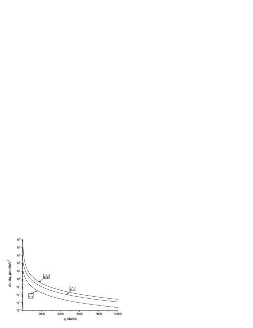
Fig. 1: The distributions $\mathrm{d}\sigma^{i}/\mathrm{d}q$ in units of pbn MeV^-1 for the cases of $\mathrm{e}^{+}\mathrm{e}^{-}$ pair, $\mu^{+}\mu^{-}$ pair and $\pi^{+}\pi^{-}$ pair production as function of $q$.

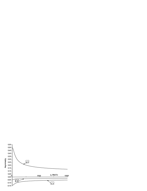
Fig. 2: Asymmetry $\Lambda^{i}$ for the cases of $\mathrm{e}^{+}\mathrm{e}^{-}$ pair, $\mu^{+}\mu^{-}$ pair and $\pi^{+}\pi^{-}$ pair production as function of $q$.

I Discussion

From the figures (2, 3) one can see that in the inclusive setup of the process of charged pairs production by interaction of linearly polarized high energy photon with proton distribution of recoil proton has rather essential azimuthal asymmetry, from 0.02 at the relatively small polar angles $\theta$ up to $\Lambda_{tot}\sim 0.05$ at $\theta\sim\pi/2$.

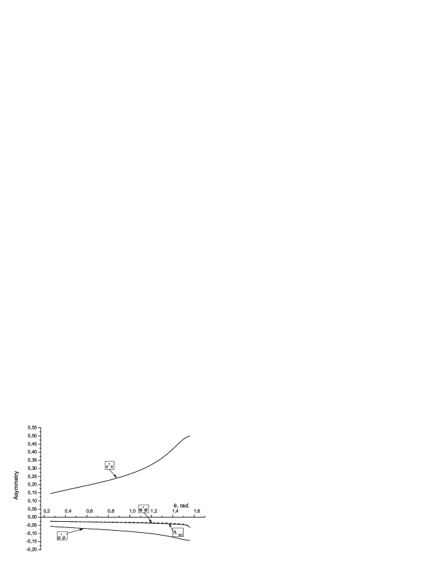
Fig. 3: Asymmetry $\Lambda^{i}$ for the cases of $\mathrm{e}^{+}\mathrm{e}^{-}$ pair, $\mu^{+}\mu^{-}$ pair and $\pi^{+}\pi^{-}$ pair production and also $\Lambda_{tot}$ as function of scattering angle $\theta$.

In exclusive setup for processes with more heavy particles than e⁺e^-, mentioned asymmetry increases. Particularly interesting is the process of $\pi^{+}\pi^{-}$ pair photoproduction. One can see that azimuthal asymmetry of recoil proton in this process reaches the value $\Lambda^{\pi}\sim 0.5$ at the region of small transferred momentum or for polar angles close to the value $\theta\sim\pi/2$. This features of $\pi^{+}\pi^{-}$ pair photoproduction process allows one to hope that this process can be considered as the polarimetric process. We shall discuss this process from this point of view in the more details in the next work.

The inclusive on recoil proton distribution is the sum on all possible channels including fermion ($\mathrm{e}^{+}\mathrm{e}^{-}$, $\mu^{+}\mu^{-}$, $\tau^{+},\tau^{-}$) and pseudoscalar meson ($\pi^{+}\pi^{-}$, $\mathrm{K}^{+}\mathrm{K}^{-}$) pairs. Production of heavy resonances such as $\rho^{\pm}$ meson can be excluded using experimental cuts.

The suggested method of measuring the recoil distributions can provide the independent way to control the luminosity and polarization properties of photon beam.

In paper VK the photoproduction of electron–positron pair on electron was considered in lowest order of PT. The radiative corrections to cross section were considered in paper VKM and in all orders of PT on parameter $Z\alpha$ in paper IM – both for unpolarized case. It turns that for $Z<6$ our results can be applied for photoproduction on nuclei with relevant modification of $F(q^{2})$. The radiative corrections can change the values $a^{i}$, $b^{i}/a^{i}$ in frames of 1–2$\%$.

The proton recoil momentum measurements can as well be arranged in $\mathrm{ep}\to X_{\mathrm{ep^{\prime}}}$ and $\mathrm{pp}\to X_{\mathrm{pp^{\prime}}}$ experiments with initial proton at rest. Using the Weizsäcker–Williams approximation the corresponding cross sections can be written as

$$\mathrm{d}\sigma^{\mathrm{ep}\to X_{\mathrm{ep^{\prime}}}}=\frac{2\alpha}{\pi}\int\limits_{2m}^{s/(2M)}\frac{\mathrm{d}\omega}{\omega}\big{[}\ln\frac{s}{2\omega m_{\mathrm{e}}}-\frac{1}{2}\big{]}\mathrm{d}\sigma^{\gamma\mathrm{p}\to a\bar{a}\mathrm{p^{\prime}}}$$ (14)

for electron–proton collisions and

$$\mathrm{d}\sigma^{\mathrm{pp}\to X_{\mathrm{pp^{\prime}}}}=\frac{2\alpha}{\pi}\int\limits_{2m}^{s/(2M)}\frac{\mathrm{d}\omega}{\omega}\big{[}\ln\frac{s}{2M\omega}-\frac{1}{2}\big{]}\mathrm{d}\sigma^{\gamma\mathrm{p}\to a\bar{a}\mathrm{p^{\prime}}},$$ (15)

for proton–proton collisions with $s=2EM$, $E$ is the energy of initial electron or proton and $\mathrm{d}\sigma^{\gamma\mathrm{p}\to a\bar{a}\mathrm{p^{\prime}}}$ are given above. Inferring these formulae we supposed that the transversal momentum of projectile (e or p) does not exceed $M$. The polarization vector of virtual photon interacting with proton at rest is directed along this projectile transverse momentum.

II Acknowledgements

One of us (EAK) is grateful to Institute of Physics, SAS. We are grateful to participants of seminar of theoretical physics SAS. One of us (Y.P) is grateful to Grant STSU-3239. The work was partly supported also by Slovak Grant Agency for Sciences VEGA, grant No. 2/4099/26.

Appendix A

More exact formula which takes into account power corrections for recoil proton momentum has a form BMPV

$$p=M\frac{(s-M^{2})(s-s_{1}-m^{2})\cos\theta\pm(s+M^{2})\sqrt{D_{1}}}{4M^{2}s+(s-M^{2})^{2}\sin^{2}\theta};$$ (16)

$$D_{1}=(s-s_{1}+m^{2})^{2}-4M^{2}s-(s-M^{2})^{2}\sin^{2}\theta.$$

Under condition $s\gg M^{2}$ upper branch of (16) passes to

$$p=M\biggl{(}\frac{2\cos\theta}{\sin^{2}\theta}-\frac{M^{2}}{s}\frac{(1+\cos^{2}\theta)(1+3\cos^{2}\theta)}{\cos\theta\sin^{4}\theta}$$ (17)

$$-\frac{(s_{1}-4m^{2})}{s}\frac{(1+\cos^{2}\theta)}{\cos\theta\sin^{2}\theta}+O\bigl{(}\frac{M^{4}}{s^{2}},\frac{s_{1}^{2}}{s^{2}}\bigr{)}\biggr{)},$$

with $s_{1}$ – invariant mass squared of pair produced.