Rome1-1442/06

IFIC/06-31

RM3-TH/06-24

IFUM-880-FT

hep-ph/0611266

Analytic Results for Virtual QCD Corrections
to Higgs Production and Decay
U. Aglietti, Dipartimento di Fisica, Università di Roma “La Sapienza” and INFN, Sezione di Roma, P.le Aldo Moro 2, I-00185 Rome, Italy R. Bonciani, Departament de Física Teòrica, IFIC, CSIC – Universitat de València,
E-46071 València, Spain G. Degrassi, Dipartimento di Fisica, Università di Roma Tre and INFN, Sezione di Roma Tre,
Via della Vasca Navale 84, I-00146 Rome, Italy A. Vicini Dipartimento di Fisica, Università di Milano and INFN, Sezione di Milano,
Via Celoria 16, I–20133 Milano, Italy

We consider the production of a Higgs boson via gluon-fusion and its decay into two photons. We compute the NLO virtual QCD corrections to these processes in a general framework in which the coupling of the Higgs boson to the external particles is mediated by a colored fermion and a colored scalar. We present compact analytic results for these two-loop corrections that are expressed in terms of Harmonic Polylogarithms. The expansion of these corrections in the low and high Higgs mass regimes, as well as the expression of the new Master Integrals which appear in the reduction of the two-loop amplitudes, are also provided. For the fermionic contribution, we provide an independent check of the results already present in the literature concerning the Higgs boson and the production and decay of a pseudoscalar particle.

Key words: Feynman diagrams, Multi-loop calculations, Higgs physics

PACS: 11.15.Bt; 12.38.Bx; 13.85.Lg; 14.80.Bn; 14.80.Cp.

1 Introduction

The Higgs searches program at the TEVATRON and at the LHC requires from the theoretical side the highest possible level of accuracy in the prediction of the production cross-sections and of all the decay channels. Over the years a lot of effort has been devoted to the study of the QCD, and also EW, corrections to the various production mechanisms and decays in the Standard Model and beyond (for a recent review see Ref.[1]).

The gluon-fusion process $gg\to H+X$ [2] is the dominant production mechanism. Its present knowledge includes the NLO [3, 4, 5] and NNLO QCD corrections [6] and the two-loop EW corrections [7, 8, 9]. The QCD corrections to Higgs production at finite transverse momentum have also been discussed [10]. While the NLO QCD corrections and the two-loop EW light fermion contribution are known completely, namely for arbitrary value of the Higgs mass and of the other relevant particles in the loops, the NNLO QCD corrections are only known in the heavy top limit while the result for the two-loop EW top contribution is valid only for intermediate Higgs mass, i.e. $m_{\scriptscriptstyle H}\leq 2m_{\scriptscriptstyle W}$.

The Higgs decay $H\to\gamma\gamma$ [11] is, for light values of the boson mass, a very promising channel. It has been studied in great detail including the NLO QCD [12, 13] and the two-loop EW corrections [14, 8, 15, 16]. The NLO QCD corrections are now known in a closed analytic form [13, 5], while for the EW corrections their knowledge is similar to that of the gluon fusion process.

Given the importance of the Higgs physics program, it is highly desirable to have the radiative corrections to the various reactions expressed in analytic form that can be easily implemented in computer codes. With respect to this, it should be recalled that the complete result concerning the NLO QCD corrections to the gluon fusion process has been reported in Ref.[4] via a rather lengthy formula expressed in terms of a one-dimensional integral representation. Actually the calculation of the two-loop light-fermion EW corrections to the Higgs production and decay [8] has shown that corrections of this kind can be calculated analytically, expressing the results in terms of Harmonic Polylogarithms (HPL) [17], a generalization of Nielsen’s polylogarithms, and an extension of the HPL, the so-called Generalized Harmonic Polylogarithms (GHPL) [18]. The idea lying behind the introduction of (G)HPLs is to express a given integral coming from the calculation of a Feynman diagram in a unique and non-redundant way as a linear combination of a minimal set of independent transcendental functions. These functions are expressed as repeated integrations over a starting set of basis functions and this set depends strongly on the problem one has to solve, being connected directly to the threshold structure of the diagrams under consideration.

An inspection of the threshold structure of the NLO QCD corrections to the gluon-fusion process and to $H\to\gamma\gamma$ decay shows that these corrections can be fully expressed in terms of the original set of HPLs introduced in [17]. A FORTRAN program [19] and a Mathematica package [20] that efficiently evaluate these functions are available.

The aim of this paper is to provide analytic expressions, in terms of HPLs, for the NLO QCD corrections to the Higgs production cross section via gluon fusion, i.e. $gg\to H$, in a general form that can be applied both to the SM and to models beyond it, and, moreover, to provide an independent check for the formulas already present in the literature. The production mechanism is assumed to be mediated by colored fermion and scalar particles. As a byproduct we also present the NLO QCD corrections to the Higgs decay into two photons, i.e. $H\to\gamma\gamma$. A similar project has been carried out in Ref.[5]. There, the authors started from the result of Ref.[4] expressed as a one-dimensional integral representation. Expanding this result in a power series, employing the theorem that two analytic functions are the same if their Taylor series are the same, they were able to rewrite it in terms of HPLs. In our case we explicitly compute all the relevant Feynman diagrams, expressing the result in term of HPLs. The calculational techniques we employed are the Laporta algorithm [21] for the reduction to Master Integrals (MIs) and the differential equation method [22] for their calculation (the calculation is implemented in FORM [23] codes). To complete an independent check of the results presented in Ref.[4] we also computed the NLO QCD corrections to the pseudoscalar production and decay, i.e. $gg\to A,\>A\to\gamma\gamma$.

The paper is organized as follows: in Section 2 we discuss the QCD corrections to the decay width $H\to\gamma\gamma$. Section 3 is devoted to the study of the Higgs production via the gluon fusion mechanism. The following section contains the analytic expressions for the virtual QCD corrections to the fermionic contribution in $gg\to A,\>A\to\gamma\gamma$. Finally we present our conclusions. We include also two Appendices. In the first one we collect the expansions of the relevant functions in the two regimes: for Higgs mass much lighter than the particles mediating the Higgs interaction with the vector bosons and in the opposite case. In the second Appendix we collect the MIs not already present in the literature, that enters the calculation of the NLO QCD corrections.

2 The $H\to\gamma\gamma$ Decay Width

We begin by considering the decay width $H\to\gamma\gamma$. Being the Higgs boson electrically neutral its coupling to the photon is mediated at the loop-level by charged particles. For the latters we assume a vector boson neutral under $SU(N_{c})$, a fermion and a scalar particle in a generic $R_{1/2},\,R_{0}$ $SU(N_{c})$ representation, respectively, whose coupling’s strengths to the Higgs are:

$$HVV=g\,\lambda_{1}\,m_{\scriptscriptstyle W},~{}~{}~{}~{}~{}~{}~{}~{}~{}~{}~{}HFF=g\,\lambda_{1/2}\,\frac{m_{1/2}}{2\,m_{\scriptscriptstyle W}},~{}~{}~{}~{}~{}~{}~{}~{}~{}~{}~{}HSS=g\,\lambda_{0}\,\frac{A^{2}}{m_{\scriptscriptstyle W}}~{},$$ (1)

where $g$ is the $SU(2)$ coupling, $m_{\scriptscriptstyle W}$ is the W mass, $m_{1/2}$ is the fermion mass, $A$ is a generic coupling with the dimension of mass and $\lambda_{i}$ are numerical coefficients.

The partial decay width for the reaction $H\to\gamma\gamma$ can be written as:

$$\Gamma(H\to\gamma\gamma)=\frac{G_{\mu}\alpha^{2}m_{H}^{3}}{128\sqrt{2}\pi^{3}}\left|{\mathcal{F}}\right|^{2}~{},$$ (2)

where the function ${\mathcal{F}}$ can be organized with respect to the lowest order term and its QCD corrections as:

$${\mathcal{F}}=\lambda_{1}\,Q_{1}^{2}\,N_{1}\,{\mathcal{F}}_{1}+\lambda_{1/2}\,Q_{1/2}^{2}\,N_{1/2}{\mathcal{F}}_{1/2}+\lambda_{0}\,Q_{0}^{2}\,N_{0}\frac{A^{2}}{m_{0}^{2}}\,{\mathcal{F}}_{0}\,,$$ (3)

where $m_{0}$ is the mass of the scalar particle, while $Q_{i}$ and $N_{i}$, $i=0,1/2,1$, are the electric charges and the representation numbers under $SU(N_{c})$ of the scalar, fermion and vector boson particles, respectively.

Writing:

$${\mathcal{F}}_{i}={\mathcal{F}}^{(1l)}_{i}+{\mathcal{F}}^{(2l)}_{i}+\dots$$ (4)

we have at the one-loop level

$${\mathcal{F}}^{(1l)}_{1} = 2(1+6y_{1})-12y_{1}(1-2y_{1})\,H(0,0,x_{1})\,,$$ (5)

$${\mathcal{F}}^{(1l)}_{1/2} = -4y_{1/2}\left[2-\left(1-4y_{1/2}\right)\,H(0,0,x_{1/2})\right]\,,$$ (6)

$${\mathcal{F}}^{(1l)}_{0} = 4y_{0}\left[1+2\,y_{0}\,H(0,0,x_{0})\right]~{}.$$ (7)

In Eqs.(5-7)

$$y_{i}\equiv\frac{m_{i}^{2}}{m_{\scriptscriptstyle H}^{2}},~{}~{}~{}~{}~{}~{}~{}~{}x_{i}\equiv\frac{\sqrt{1-4y_{i}}-1}{\sqrt{1-4y_{i}}+1}\,,$$ (8)

with $m_{1}$ the mass of the vector particle and, employing the standard notation for the HPLs, $H(0,0,z)$ labels a HPL of weight 2 that results to be

$$H(0,0,z)=\frac{1}{2}\log^{2}(z)~{}.$$ (9)

The QCD corrections to the lowest order result can be written as

$${\mathcal{F}}_{QCD}^{(2l)}=\frac{\alpha_{s}}{\pi}\sum_{i=(0,1/2)}C(R_{i})\,{\mathcal{F}}_{i}^{(2l)}\,,$$ (10)

where $C(R)$ is the Casimir factor of the $R_{i}$ representation (in particular, for the fundamental and the adjoint representations of $SU(N_{c})$ we have $C_{F}=(N_{c}^{2}-1)/(2N_{c})$ and $C_{A}=N_{c}$, respectively). We consider first the fermion contribution (the relevant Feynman diagrams are shown in Fig. 1 (a)–(d)).

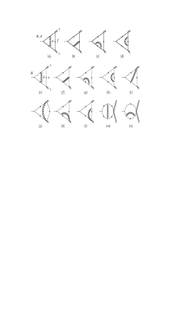
Figure 1: The Feynman diagrams for the decay process $H,A\to\gamma\gamma$. Diagrams (a)–(d) have a fermion, labeled by “f”, running in the loop, while diagrams (e)–(n) have a scalar, labeled by “s”.

The expression for ${\mathcal{F}}_{1/2}^{(2l)}$ depends upon the renormalized mass parameter employed. In the case of $\overline{\mbox{MS}}$ quark masses we have

$${\mathcal{F}}_{1/2}^{(2l)}={\mathcal{F}}_{1/2}^{(2l,a)}(x_{1/2})+{\mathcal{F}}_{1/2}^{(2l,b)}(x_{1/2})\ln\left({m_{1/2}^{2}\over\mu^{2}}\right)\,,$$ (11)

where $\mu$ is the ’t Hooft mass and

$${\mathcal{F}}_{1/2}^{(2l,a)}(x) = \frac{36x}{(x-1)^{2}}-\frac{4x\left(1-14x+x^{2}\right)}{(x-1)^{4}}\,\zeta_{3}-\frac{4x(1+x)}{(x-1)^{3}}\,H(0,x)$$ (12)

$$-\frac{8x\left(1+9x+x^{2}\right)}{(x-1)^{4}}\,H(0,0,x)+\frac{2x\left(3+25x-7x^{2}+3x^{3}\right)}{(x-1)^{5}}\,H(0,0,0,x)$$

$$+\frac{4x\left(1+2x+x^{2}\right)}{(x-1)^{4}}\,\bigl{[}\zeta_{2}H(0,x)+4\,H(0,-1,0,x)-H(0,1,0,x)\bigr{]}$$

$$+\frac{4x\left(5-6x+5x^{2}\right)}{(x-1)^{4}}\,H(1,0,0,x)-\frac{8x\left(1+x+x^{2}+x^{3}\right)}{(x-1)^{5}}\,{\mathcal{H}}_{1}(x)\,,$$

$${\mathcal{F}}_{1/2}^{(2l,b)}(x) = -\frac{12x}{(x-1)^{2}}-\frac{6x(1+x)}{(x-1)^{3}}\,H(0,x)+\frac{6x\left(1+6x+x^{2}\right)}{(x-1)^{4}}\,H(0,0,x)\,,$$ (13)

with

$${\mathcal{H}}_{1}(x) = \frac{9}{10}{\zeta_{2}}^{2}+2\zeta_{3}H(0,x)+\zeta_{2}H(0,0,x)+\frac{1}{4}\,H(0,0,0,0,x)+\frac{7}{2}\,H(0,1,0,0,x)$$ (14)

$$-2\,H(0,-1,0,0,x)+4\,H(0,0,-1,0,x)-H(0,0,1,0,x)\,.$$

In Eqs.(12,14) $\zeta_{n}\equiv\zeta(n)$ are the Riemann’s zeta functions.

The expression for ${\mathcal{F}}_{1/2}^{(2l)}$ in case the one-loop result is given in terms of on-shell fermion masses is given instead by:

$${\mathcal{F}}_{1/2}^{(2l)}={\mathcal{F}}_{1/2}^{(2l,a)}(x_{1/2})+\frac{4}{3}{\mathcal{F}}_{1/2}^{(2l,b)}(x_{1/2})~{}.$$ (15)

Eq.(15) is in agreement with the results presented in [13, 5].

We now present the scalar contribution, ${\mathcal{F}}_{0}^{(2l)}$, assuming that both the mass of the scalar, $m_{0}$, and the coupling $A$ are renormalized in the $\overline{\mbox{MS}}$ scheme (the relevant Feynman diagrams are shown in Fig. 1 (e)–(n)). We find

$${\mathcal{F}}_{0}^{(2l)}={\mathcal{F}}_{0}^{(2l,a)}(x_{0})+\left({\mathcal{F}}_{0}^{(2l,b)}(x_{0})+{\mathcal{F}}_{0}^{(2l,c)}(x_{0})\right)\ln\left({m_{0}^{2}\over\mu^{2}}\right)\,,$$ (16)

where

$${\mathcal{F}}_{0}^{(2l,a)}(x) = -\frac{14x}{(x-1)^{2}}-\frac{24x^{2}}{(x-1)^{4}}\,\zeta_{3}+\frac{x\left(3-8x+3x^{2}\right)}{(x-1)^{3}(x+1)}\,H(0,x)+\frac{34x^{2}}{{\left(x-1\right)}^{4}}\,H(0,0,x)$$ (17)

$$-\frac{8x^{2}}{(x-1)^{4}}\,\bigl{[}\zeta_{2}H(0,x)+4H(0,-1,0,x)-H(0,1,0,x)+H(1,0,0,x)\bigr{]}$$

$$-\frac{2x^{2}(5-11x)}{(x-1)^{5}}\,H(0,0,0,x)+\frac{16x^{2}\left(1+x^{2}\right)}{(x-1)^{5}(x+1)}\,{\mathcal{H}}_{1}(x)\,,$$

$${\mathcal{F}}_{0}^{(2l,b)}(x) = \frac{6x^{2}}{(x-1)^{3}(x+1)}\,H(0,x)-\frac{6x^{2}}{(x-1)^{4}}\,H(0,0,x)\,,$$ (18)

$${\mathcal{F}}_{0}^{(2l,c)}(x) = -\frac{3}{4}\,{\mathcal{F}}_{0}^{(1l)}\,.$$ (19)

We provide also ${\mathcal{F}}_{0}^{(2l)}$ assuming that the mass of the scalar is renormalized on-shell while the $A$ coupling is still given as an $\overline{\mbox{MS}}$ one. It reads

$${\mathcal{F}}_{0}^{(2l)}={\mathcal{F}}_{0}^{(2l,a)}(x_{0})+\frac{7}{3}\,{\mathcal{F}}_{0}^{(2l,b)}(x_{0})+{\mathcal{F}}_{0}^{(2l,c)}(x_{0})\ln\left({m_{0}^{2}\over\mu^{2}}\right)~{}.$$ (20)

3 Virtual Corrections to $gg\to H$ Production Mechanism

In this section we present the analytic expressions for the virtual two-loop QCD corrections for Higgs boson production via the gluon fusion mechanism. Being the Higgs boson neutral under $SU(N_{c})$, its coupling to the gluons is mediated by a loop of colored particles. As in Section 2, we consider a fermion and a scalar particle, that run in the loops. The Feynman diagrams relevant for the NLO corrections to the production cross section are shown in Fig. 2.

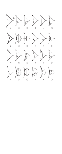
Figure 2: The Feynman diagrams for the production mechanism $gg\to H,A$. Diagrams (a)–(h) have a fermion, labeled by “f”, running in the loop, while diagrams (i)–(x) have a scalar, labeled by “s”.

The hadronic cross section can be written as:

$$\sigma(h_{1}+h_{2}\to H+X) = \sum_{a,b}\int_{0}^{1}dx_{1}dx_{2}\,\,f_{a,h_{1}}(x_{1},\mu_{F}^{2})\,f_{b,h_{2}}(x_{2},\mu_{F}^{2})\times$$ (21)

$$\times\int_{0}^{1}dz~{}\delta\left(z-\frac{\tau_{H}}{x_{1}x_{2}}\right)\hat{\sigma}_{ab}(z)\,,$$

where $\tau_{H}=m_{\scriptscriptstyle H}^{2}/s$, $\mu_{F}$ is the factorization scale, $f_{a,h_{i}}(x,\mu_{F}^{2})$, the parton density of the colliding hadron $h_{i}$ for the parton of type $a,\,(a=g,q,\bar{q})$ and $\hat{\sigma}_{ab}$ the cross section for the partonic subprocess $ab\to H+X$ at the center-of-mass energy $\hat{s}=x_{1}x_{2}s=m_{\scriptscriptstyle H}^{2}/z$. The latter can be written as:

$$\hat{\sigma}_{ab}(z)=\sigma^{(0)}\,z\,G_{ab}(z)\,,$$ (22)

where

$$\sigma^{(0)}=\frac{G_{\mu}\alpha_{s}^{2}(\mu_{R}^{2})}{128\,\sqrt{2}\,\pi}\left|\sum_{i=0,1/2}\lambda_{i}\left(\frac{A^{2}}{m_{0}^{2}}\right)^{1-2i}\,T(R_{i})\,{\mathcal{G}}^{(1l)}_{i}\right|^{2}$$ (23)

is the Born-level contribution with ${\mathcal{G}}^{(1l)}_{i}={\mathcal{F}}^{(1l)}_{i}$ and $T(R_{i})$ are the matrix normalization factors of the $R_{i}$ representation ($T(R)=1/2$ for the fundamental representation of $SU(N_{c})$, $T(R)=N_{c}$ for the adjoint one).

Up to NLO contributions we can write

$$G_{ab}(z)=G_{ab}^{(0)}(z)+\frac{\alpha_{s}(\mu^{2}_{R})}{\pi}\,G_{a,b}^{(1)}(z)\,,$$ (24)

with

$$G_{ab}^{(0)}(z) = \delta(1-z)\,\delta_{ag}\,\delta_{bg}\,,$$ (25)

$$G_{gg}^{(1)}(z) = \delta(1-z)\left[C_{A}\,\frac{\pi^{2}}{3}+\beta_{0}\ln\left(\frac{\mu_{R}^{2}}{\mu_{F}^{2}}\right)+\sum_{i=0,1/2}{\mathcal{G}}^{(2l)}_{i}\right]+\dots$$ (26)

The dots in Eq.(26) represent the contribution from the real emission that we have not written as well as the other NLO factors $G_{gq}^{(1)}(z),\,G_{qq}^{(1)}(z),\,G_{q\bar{q}}^{(1)}(z)$. In Eq.(26) $\beta_{0}=(11\,C_{A}-4\,n_{f}\,T(R_{f})-n_{s}\,T(R_{s})/6$ with $n_{f}\>(n_{s})$ the number of active fermion (scalar) flavor in the representation $R_{f}\>(R_{s})$.

The function ${\mathcal{G}}^{(2l)}_{i}$ can be cast in the following form:

$${\mathcal{G}}^{(2l)}_{i} = \lambda_{i}\left(\frac{A^{2}}{m_{0}^{2}}\right)^{1-2i}\,T(R_{i})\Biggl{(}C(R_{i})\,{\mathcal{G}}^{(2l,C_{R})}_{i}(x_{i})+C_{A}\,{\mathcal{G}}^{(2l,C_{A})}_{i}(x_{i})\Biggr{)}$$ (27)

$$\times\left(\sum_{j=0,1/2}\lambda_{j}\left(\frac{A^{2}}{m_{0}^{2}}\right)^{1-2j}\,T(R_{j})\,{\mathcal{G}}^{(1l)}_{j}\right)^{-1}+h.c.$$

with ${\mathcal{G}}^{(2l,C_{R})}_{i}={\mathcal{F}}^{(2l)}_{i}$. The infrared regularized functions ${\mathcal{G}}^{(2l,C_{A})}_{i}$, after subtraction of the infrared poles, are found to be:

$${\mathcal{G}}^{(2l,C_{A})}_{1/2}(x) = \frac{4x}{(x-1)^{2}}\Biggl{[}\,3+\frac{x(1+8x+3x^{2})}{(x-1)^{3}}\,H(0,0,0,x)-\frac{2(1+x)^{2}}{(x-1)^{2}}\,{\mathcal{H}}_{2}(x)$$ (28)

$$\hskip 61.17342pt+\,\zeta_{3}-H(1,0,0,x)\Biggr{]},$$

$${\mathcal{G}}^{(2l,C_{A})}_{0}(x) = \frac{4x}{(x-1)^{2}}\Biggl{[}-\frac{3}{2}+\frac{x(1-7x)}{(x-1)^{3}}H(0,0,0,x)+\frac{4x}{(x-1)^{2}}{\cal H}_{2}(x)\Biggr{]}\,,$$ (29)

with

$${\cal H}_{2}(x) = \frac{4}{5}{\zeta_{2}}^{2}+2\zeta_{3}+\frac{3\zeta_{3}}{2}\,H(0,x)+3\zeta_{3}H(1,x)+\zeta_{2}H(1,0,x)+\frac{1}{4}\left(1+2\zeta_{2}\right)\,H(0,0,x)$$ (30)

$$-2\,H(1,0,0,x)+H(0,0,-1,0,x)+\frac{1}{4}H(0,0,0,0,x)+2\,H(1,0,-1,0,x)$$

$$-H(1,0,0,0,x)\,.$$

The analytic expression of ${\mathcal{G}}^{(2l)}_{1/2}$ is in agreement with that reported in Ref.[5] based on the results presented in Ref.[4].

4 Pseudoscalar Higgs: $A\to\gamma\gamma$ and $gg\to A$

To complete an independent check of the results of Ref.[4] in this section we consider the virtual NLO QCD corrections to the decay width of a pseudo-scalar particle $A$ in two photons, $\Gamma(A\to\gamma\gamma)$, and to its production cross section via gluon fusion, $\hat{\sigma}(gg\to A)$.

As in Ref.[4] we assume the interaction of the $A$ particle with gluons mediated only by the top quark. Because the NLO QCD corrections to these two processes are calculated in Dimensional Regularization, a prescription for the $\gamma_{5}$ matrix is needed. We use the same prescription of Ref.[4], i.e. ’t Hooft–Veltman one [24], that, as it is well known, breaks manifestly Ward Identities. The latters need to be restored explicitly, with a finite renormalization. If $Z_{Hf\bar{f}}$ and $Z_{Af\bar{f}}$ are the renormalization constants of the vertex $Hf\bar{f}$, scalar Higgs-fermion-antifermion, and $Af\bar{f}$, pseudo-scalar Higgs-fermion-antifermion, respectively, the contribution of the finite renormalization can be found using [4, 25]:

$$Z_{Af\bar{f}}=Z_{Hf\bar{f}}+2C_{F}\frac{\alpha_{S}}{\pi}\,.$$ (31)

4.1 Decay Width $A\to\gamma\gamma$

In analogy with Eq.(2), we write:

$$\Gamma(A\to\gamma\gamma)=\frac{G_{\mu}\alpha^{2}m_{A}^{3}}{128\sqrt{2}\pi^{3}}\left|{\mathcal{E}}\right|^{2}~{}.$$ (32)

Assuming the strength of the coupling of the pseudoscalar to the top quark equal to $Att=g\,\eta_{t}\,m_{t}/(2\,m_{\scriptscriptstyle W})$, with $m_{t}$ the top mass and $\eta_{t}$ a numerical coefficient, the function ${\mathcal{E}}$ can be written as ($Q_{t}=2/3$):

$${\mathcal{E}}=\eta_{t}\,Q_{t}^{2}\,N_{c}\Bigl{[}{\mathcal{E}}^{(1l)}_{t}+\frac{\alpha_{S}}{\pi}C_{F}{\mathcal{E}}^{(2l)}_{t}+\dots\Bigr{]}\,.$$ (33)

The leading order term is

$${\mathcal{E}}^{(1l)}_{t}=4\,y_{t}H(0,0,x_{t})\,,$$ (34)

where $y_{t}$, $x_{t}$ are given by Eq.(8) with $i=t$. At the NLO, assuming an $\overline{\mbox{MS}}$ top mass we have:

$${\mathcal{E}}^{(2l)}_{t}={\mathcal{E}}_{t}^{(2l,a)}(x_{t})+{\mathcal{E}}_{t}^{(2l,b)}(x_{t})\ln\left({m_{t}^{2}\over\mu^{2}}\right)\,,$$ (35)

where:

$${\mathcal{E}}_{t}^{(2l,a)}(x) = -\frac{4x}{(x-1)^{2}}\bigl{[}\zeta_{3}-4H(0,-1,0,x)+H(0,1,0,x)-5H(1,0,0,x)\bigr{]}$$ (36)

$$+\frac{4x\left[2(1-x)^{2}-\zeta_{2}(1-x^{2})\right]}{(x-1)^{3}(1+x)}H(0,x)+\frac{8x(1-x^{2})}{(x-1)^{3}(1+x)}H(0,0,x)$$

$$+\frac{6x(1+x)}{(x-1)^{3}}H(0,0,0,x)-\frac{8x(1+x^{2})}{(x-1)^{3}(1+x)}{\mathcal{H}}_{1}\,,$$

$${\mathcal{E}}_{t}^{(2l,b)}(x) = -\frac{6x}{(x-1)(1+x)}H(0,x)+\frac{6x}{(x-1)^{2}}H(0,0,x)\,.$$ (37)

The corresponding expression for an OS top mass is given by:

$${\mathcal{E}}_{t}^{(2l)}={\mathcal{E}}_{t}^{(2l,a)}(x_{t})+\frac{4}{3}{\mathcal{E}}_{t}^{(2l,b)}(x_{t})~{}.$$ (38)

4.2 Production Cross Section $gg\to A$

The expressions for the relevant quantities in the $gg\to A$ production cross section can be easily obtained from those in Section 3, with the substitutions: $T(R_{i})\to 1/2,\>C(R_{i})\to C_{F},\>{\mathcal{F}}\to{\mathcal{E}},\>{\mathcal{G}}\to{\mathcal{K}}$. In particular, the Born-level partonic cross section (Eq.(23)) is:

$$\sigma^{(0)}=\frac{G_{\mu}\alpha_{s}^{2}(\mu_{R}^{2})}{128\,\sqrt{2}\,\pi}\left|\frac{1}{2}\eta_{t}\,{\mathcal{K}}^{(1l)}_{t}\right|^{2}\,,$$ (39)

with ${\mathcal{K}}^{(1l)}_{t}={\mathcal{E}}^{(1l)}_{t}$. The NLO virtual contribution to the gluon fusion subprocess (Eq.(26)) is:

$$G_{gg}^{(1)}(z)=\delta(1-z)\left[C_{A}\,\frac{\pi^{2}}{3}+\beta_{0}\ln\left(\frac{\mu_{R}^{2}}{\mu_{F}^{2}}\right)+{\mathcal{K}}^{(2l)}_{t}\right]\,,$$ (40)

where $\beta_{0}=(11\,C_{A}-2\,n_{f})/6$, with $n_{f}$ the number of active flavor, and

$${\mathcal{K}}^{(2l)}_{t}=\left({\mathcal{K}}^{(1l)}_{t}\right)^{-1}\Biggl{(}C_{F}\,{\mathcal{K}}^{(2l,C_{F})}_{t}(x_{t})+C_{A}\,{\mathcal{K}}^{(2l,C_{A})}_{t}(x_{t})\Biggr{)}+h.c.$$ (41)

with ${\mathcal{K}}^{(2l,C_{F})}_{t}={\mathcal{E}}^{(2l)}_{t}$ and

$${\mathcal{K}}^{(2l,C_{A})}_{t}(x)=\frac{4x}{(x-1)^{2}}\bigl{[}\zeta_{3}-H(1,0,0,x)-2{\mathcal{H}}_{2}(x)\bigr{]}+\frac{12x^{2}}{(x-1)^{3}}H(0,0,0,x)\,.$$ (42)

Eqs.(38,41) are in agreement with the corresponding expressions presented in Ref.[5].

5 Conclusions

In this paper, we considered the virtual NLO QCD corrections to the processes $H\to\gamma\gamma$ and $gg\to H$. We assumed the coupling of the Higgs boson to the photons and gluons to be mediated by fermionic and scalar loops. We provided analytic formulas for these corrections that are valid for arbitrary mass of the fermion or scalar particle running in the loops and of the Higgs boson. They are given in a very compact form as a combination of HPLs.

The calculation here presented was done using the Laporta algorithm for the reduction of the scalar integrals to the MIs and the differential equations method for the evaluation of the latters. A part of the MIs needed for the calculation was already known in the literature. We explicitly give the analytic results for the MIs that were not known.

We checked our results for the decay width of the Higgs boson in two photons and for the partonic cross section of the gluon fusion by performing an independent calculation in the region of small Higgs mass via an asymptotic expansion in the variable $r\equiv m_{\scriptscriptstyle H}^{2}/m^{2}\ll 1$, with $m$ the mass of the fermion or scalar particle, up to the first 4-5 orders.

We considered also the NLO virtual QCD corrections to $A\to\gamma\gamma$ and $gg\to A$ assuming the coupling of the pseudoscalar boson to the external particles mediated by a fermion.

We find complete agreement with the results previously known in the literature concerning the production and decay of a (pseudo)scalar Higgs boson mediated by fermionic loops. This provides an independent check of the formulas given in Refs.[4, 5] and extends them to the case of a scalar particle running in the loops.

Acknowledgments

The authors want to thank M. Spira and A. Djouadi for useful communications regarding Ref.[4]. R. B. wishes to thank the Department of Physics of the University of Florence and INFN Section of Florence for kind hospitality, and in particular S. Catani for useful discussions during a large part of this work. Discussions with G. Rodrigo are gratefully acknowledged. The work of R. B. was partially supported by Ministerio de Educación y Ciencia (MEC) under grant FPA2004-00996, Generalitat Valenciana under grant GV05-015, and MEC-INFN agreement.

Note added

After our work was completed a paper on a similar subject has appeared on the Web [27]. We did not check yet our formulas against theirs.

Appendix A: Results in the Low and High Higgs Mass Regimes

In this Appendix we present approximate results that are valid in regions in which the mass of the Higgs boson is either much smaller or much larger than that of the particle running in the loop.

A.1 $H\to\gamma\gamma$

The expansions of Eqs.(5-7) with respect to $r_{i}=m_{\scriptscriptstyle H}^{2}/m_{i}^{2}$, when $r_{i}\ll 1$ read:

$${\cal F}_{1}^{(1l)}(r) = 7+\frac{11}{30}r+\frac{19}{420}r^{2}+\frac{29}{4200}r^{3}+\frac{41}{34650}r^{4}+{\mathcal{O}}\left(r^{5}\right)\,,$$ (A1)

$${\cal F}_{1/2}^{(1l)}(r) = -\frac{4}{3}-\frac{7}{90}r-\frac{1}{126}r^{2}-\frac{13}{12600}r^{3}-\frac{8}{51975}r^{4}+{\mathcal{O}}\left(r^{5}\right)\,,$$ (A2)

$${\cal F}_{0}^{(1l)}(r) = -\frac{1}{3}-\frac{2}{45}r-\frac{1}{140}r^{2}-\frac{2}{1575}r^{3}-\frac{1}{4158}r^{4}+{\mathcal{O}}\left(r^{5}\right)\,,$$ (A3)

while in the opposite case, $r_{i}\gg 1$ we find:

$${\cal F}_{1}^{(1l)}(r) = 2+\left(12-6\ln^{2}(-r)\right)\frac{1}{r}+\left(24\ln(-r)+12\ln^{2}(-r)\right)\frac{1}{r^{2}}+{\mathcal{O}}\left(\frac{1}{r^{3}}\right)\,,$$ (A4)

$${\cal F}_{1/2}^{(1l)}(r) = -\left(8-2\ln^{2}(-r)\right)\frac{1}{r}-\left(8\ln(-r)+8\ln^{2}(-r)\right)\frac{1}{r^{2}}+{\mathcal{O}}\left(\frac{1}{r^{3}}\right)\,,$$ (A5)

$${\cal F}_{0}^{(1l)}(r) = \frac{4}{r}+4\ln^{2}(-r)\frac{1}{r^{2}}+{\mathcal{O}}\left(\frac{1}{r^{3}}\right)\,.$$ (A6)

The expansions of Eqs.(15,20) when $r_{i}\ll 1$ are

$${\cal F}_{1/2}^{(2l,a)}(r) = 1-\frac{19}{270}r-\frac{104}{14175}r^{2}-\frac{6313}{15876000}r^{3}+\frac{5083}{74844000}r^{4}+{\mathcal{O}}\left(r^{5}\right),$$ (A7)

$${\cal F}_{1/2}^{(2l,b)}(r) = -\frac{7}{60}r-\frac{1}{42}r^{2}-\frac{13}{2800}r^{3}-\frac{16}{17325}r^{4}+{\mathcal{O}}\left(r^{5}\right),$$ (A8)

$${\cal F}_{0}^{(2l,a)}(r) = -\frac{3}{4}-\frac{29}{216}r-\frac{4973}{226800}r^{2}-\frac{3137}{882000}r^{3}-\frac{1180367}{2095632000}r^{4}+{\mathcal{O}}\left(r^{5}\right),$$ (A9)

$${\cal F}_{0}^{(2l,b)}(r) = -\frac{1}{4}-\frac{1}{15}r-\frac{9}{560}r^{2}-\frac{2}{525}r^{3}-\frac{5}{5544}r^{4}+{\mathcal{O}}\left(r^{5}\right),$$ (A10)

while in the opposite regime we have:

$${\cal F}_{1/2}^{(2l,a)}(r) = -\Bigl{[}36+\frac{36}{5}\zeta^{2}(2)-4\zeta(3)-4(1+\zeta(2)+4\zeta(3))\,\ln(-r)-4(1-\zeta(2))\,\ln^{2}(-r)$$ (A12)

$$+\ln^{3}(-r)+\frac{1}{12}\,\ln^{4}(-r)\Bigr{]}\frac{1}{r}-\Bigl{[}48+8\zeta(2)-\frac{144}{5}\zeta^{2}(2)-16\zeta(3)$$

$$+16(1+4\zeta(3))\,\ln(-r)+2(11-8\zeta(2))\,\ln^{2}(-r)-12\,\ln^{3}(-r)$$

$$-\frac{1}{3}\,\ln^{4}(-r)\Bigr{]}\frac{1}{r^{2}}+{\mathcal{O}}\left(\frac{1}{r^{3}}\right)\,,$$

$${\cal F}_{1/2}^{(2l,b)}(r) = \left[12+6\,\ln(-r)-3\,\ln^{2}(-r)\right]\frac{1}{r}-\left[12-24\,\ln^{2}(-r)\right]\frac{1}{r^{2}}+{\mathcal{O}}\left(\frac{1}{r^{3}}\right)\,,$$ (A13)

$${\cal F}_{0}^{(2l,a)}(r) = \left[14-3\,\ln(-r)\right]\frac{1}{r}+\Bigl{[}6-\frac{72}{5}\zeta^{2}(2)-24\zeta(3)-8(1-\zeta(2)-4\zeta(3))\,\ln(-r)$$ (A14)

$$+(17-8\zeta(2))\,\ln^{2}(-r)-\frac{5}{3}\,\ln^{3}(-r)-\frac{1}{6}\,\ln^{4}(-r)\Bigr{]}\frac{1}{r^{2}}+{\mathcal{O}}\left(\frac{1}{r^{3}}\right)\,,$$

$${\cal F}_{0}^{(2l,b)}(r) = \left[6\,\ln(-r)-3\,\ln^{2}(-r)\right]\frac{1}{r^{2}}+{\mathcal{O}}\left(\frac{1}{r^{3}}\right)\,.$$ (A15)

The imaginary part of the expressions in Eqs.(A4–A6) and (A12–A15) can be easily recovered via the substitution

$$\ln{(-r-i\epsilon)}\rightarrow\ln{r}-i\pi\,.$$ (A16)

A.2 $gg\to H$

The expansions of Eqs.(28,29) when $r_{i}\ll 1$ are

$${\cal G}^{(2l,C_{A})}_{1/2}(r) = -\frac{5}{3}-\frac{29}{1080}r-\frac{1}{7560}r^{2}+\frac{29}{168000}r^{3}+\frac{3329}{74844000}r^{4}+{\mathcal{O}}\left(r^{5}\right)\,,$$ (A17)

$${\cal G}^{(2l,C_{A})}_{0}(r) = -\frac{1}{6}-\frac{1}{135}r+\frac{1}{15120}r^{2}+\frac{29}{189000}r^{3}+\frac{1433}{29937600}r^{4}+{\mathcal{O}}\left(r^{5}\right)\,,$$ (A18)

while in the opposite regime we have:

$${\cal G}^{(2l,C_{A})}_{1/2}(r) = -\Bigl{[}12-\frac{32}{5}\zeta^{2}(2)-12\zeta(3)+12\zeta(3)\ln(-r)-(1+2\zeta(2))\ln^{2}(-r)$$ (A19)

$$-\frac{1}{12}\ln^{4}(-r)\Bigr{]}\frac{1}{r}+\Bigl{[}28+8\zeta(2)-\frac{128}{5}\zeta^{2}(2)-64\zeta(3)+8(1+6\zeta(3))\ln(-r)$$

$$-2(1+4\zeta(2))\ln^{2}(-r)-\frac{4}{3}\ln^{3}(-r)-\frac{1}{3}\ln^{4}(-r)\Bigr{]}\frac{1}{r^{2}}+{\mathcal{O}}\left(\frac{1}{r^{3}}\right)\,,$$

$${\cal G}^{(2l,C_{A})}_{0}(r) = \frac{6}{r}+\Bigl{[}\frac{64}{5}\zeta^{2}(2)+32\zeta(3)-24\zeta(3)\ln(-r)+2(1+2\zeta(2))\ln^{2}(-r)$$ (A20)

$$+\frac{2}{3}\ln^{3}(-r)+\frac{1}{6}\ln^{4}(-r)\Bigr{]}\frac{1}{r^{2}}+{\mathcal{O}}\left(\frac{1}{r^{3}}\right)\,,$$

The imaginary part of the expressions in Eqs.(A19,A20) can be easily recovered via the substitution of Eq.(A16).

A.3 $A\to\gamma\gamma$ and $gg\to A$

The expansion of the one-loop result (Eq.(34)) when $r\equiv m_{A}^{2}/m_{t}^{2}\ll 1$ is

$${\mathcal{E}}_{t}^{(1l)}(r)=-2-\frac{1}{6}r-\frac{1}{45}r^{2}-\frac{1}{280}r^{3}-\frac{1}{1575}r^{4}+{\mathcal{O}}\left(r^{5}\right)\,,$$ (A21)

while for $r\gg 1$: we have:

$${\mathcal{E}}_{t}^{(1l)}(r) = 2\ln^{2}(-r)\frac{1}{r}-8\ln(-r)\frac{1}{r^{2}}+{\mathcal{O}}\left(\frac{1}{r^{3}}\right)\,.$$ (A22)

The expansions of Eqs.(36,37) when $r\ll 1$ read

$${\mathcal{E}}_{t}^{(2l,a)}(r) = -\frac{1}{3}r-\frac{19}{360}r^{2}-\frac{3533}{453600}r^{3}-\frac{151}{141120}r^{4}+{\mathcal{O}}\left(r^{5}\right)\,,$$ (A23)

$${\mathcal{E}}_{t}^{(2l,b)}(r) = -\frac{1}{4}r-\frac{1}{15}r^{2}-\frac{9}{560}r^{3}-\frac{2}{525}r^{4}+{\mathcal{O}}\left(r^{5}\right)\,,$$ (A24)

while in the opposite regime we have:

$${\mathcal{E}}_{t}^{(2l,a)}(r) = -\Bigl{[}\frac{36}{5}\zeta_{2}^{2}-4\zeta_{3}+4(2-\zeta_{2}-4\zeta_{3})\ln(-r)-4(1-\zeta_{2})\ln^{2}(-r)+\ln^{3}(-r)$$ (A25)

$$+\frac{1}{12}\ln^{4}(-r)\Bigr{]}\frac{1}{r}-\Bigl{[}24+8\zeta_{2}+32\zeta_{3}+8(3-2\zeta_{2})\ln(-r)-22\ln^{2}(-r)$$

$$-\frac{8}{3}\ln^{3}(-r)\Bigr{]}\frac{1}{r^{2}}+{\mathcal{O}}\left(\frac{1}{r^{3}}\right)\,,$$

$${\mathcal{E}}_{t}^{(2l,b)}(r) = \Bigl{[}6\ln(-r)-3\ln^{2}(-r)\Bigr{]}\frac{1}{r}-\Bigl{[}12-24\ln(-r)\Bigr{]}\frac{1}{r^{2}}+{\mathcal{O}}\left(\frac{1}{r^{3}}\right)\,.$$ (A26)

For Eq.(42) in the limit $r\ll 1$, finally, we have:

$${\mathcal{K}}^{(2l,C_{A})}_{t}(r)=-2-\frac{1}{24}r+\frac{29}{60480}r^{3}+\frac{53}{378000}r^{4}+{\mathcal{O}}\left(r^{5}\right)\,,$$ (A27)

and for $r\gg 1$:

$${\mathcal{K}}^{(2l,C_{A})}_{t}(r) = \Bigl{[}\frac{32}{5}\zeta_{2}^{2}+12\zeta_{3}-12\zeta_{3}\ln(-r)+(1+2\zeta_{2})\ln^{2}(-r)+\frac{1}{12}\ln^{4}(-r)\Bigr{]}\frac{1}{r}$$ (A28)

$$+\Bigl{[}28+8\zeta_{2}+8\ln(-r)+2\ln^{2}(-r)\Bigr{]}\frac{1}{r^{2}}+{\mathcal{O}}\left(\frac{1}{r^{3}}\right)\,.$$

The imaginary part of the expressions in Eqs.(A25,A26,A28) can be easily recovered via the substitution of Eq.(A16).

Appendix B: Master Integrals for the Two-Loop QCD Corrections

This Appendix is devoted to the analytic expressions of the MIs involved in the calculation. They are 11, as it is shown in Fig. 3.

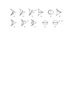
Figure 3: The Master Integrals necessary for the computation of the two-loop QCD corrections to $gg\to H$ and $H\to\gamma\gamma$.

The diagrams (e) and (g)–(k) can be found in [26]. Diagrams (a)–(d) and (f) are listed below. The integrals are performed in Euclidean $D$-dimensional space and expanded in Laurent series of $\epsilon=(2-D/2)$. The mass of the particles running in the loops is denoted by $m$, while $\mu$ is the unit of mass of the Dimensional Regularization. The variable $x$ is defined in Eq. (8).

A common prefactor of

$$\left(\frac{\mu^{2}}{m^{2}}\right)^{2\epsilon}\pi^{2(2-\epsilon)}\,\Gamma^{2}(1+\epsilon)$$ (B1)

is understood and not explicitly shown in the formulas below.

All the results of this section can be obtained in an electronic form by downloading the source files of this manuscript from http://www.arxiv.org.

B.1 Topology $t=4$

$$\hbox{ \begin{picture}(0.0,0.0)(0.0,0.0)\SetScale{.35} \SetWidth{1.5} \Photon(-60,60)(-48,50){4}{2} \Photon(-60,-60)(-48,-50){4}{2} \DashLine(20,0)(40,0){2} \Line(-48,50)(20,0) \Line(-48,-50)(20,0) \Line(-48,-50)(-48,50) \PhotonArc(12,60)(60,189,278){4}{11} \end{picture}}\hskip 17.07164pt=\sum_{i=-2}^{1}\epsilon^{i}F^{(1)}_{i}+{\mathcal{O}}\left(\epsilon^{2}\right),$$ (B2)

where:

$$F^{(1)}_{-2} = \frac{1}{2}\,,$$ (B3)

$$F^{(1)}_{-1} = \frac{1}{2}\,,$$ (B4)

$$F^{(1)}_{0} = -\frac{5}{2}-H(0,0,x)-\frac{x}{(x-1)^{2}}\bigl{[}4\zeta(3)-2H(0,0,0,x)-4H(1,0,0,x)\bigr{]}$$ (B5)

$$+\frac{2(1+x)}{(x-1)}H(0,x),$$

$$F^{(1)}_{1} = -\frac{35}{2}\!-2H(0,1,0,x)+\!\frac{1}{(x-1)^{2}}\Bigl{\{}\frac{8}{5}\zeta^{2}(2)x+\!(3x^{2}\!-\!10x\!+\!3)\zeta(3)-2(x^{2}-1)\zeta(2)$$ (B6)

$$+\!\bigl{[}12(x^{2}-1)\!+\!(x-1)^{2}\zeta(2)-\!6x\zeta(3)\bigr{]}H(0,x)-[7-2x-9x^{2}\!+\!2x\zeta(2)]H(0,0,x)$$

$$+\bigl{[}4(x^{2}-1)-4x\zeta(2)\bigr{]}H(1,0,x)-12(x^{2}-1)H(-1,0,x)-[3x^{2}-8x+3]\times$$

$$\times H(0,0,0,x)\!+\!6(x-1)^{2}H(0,-1,0,x)\!+\!2(1\!+\!x^{2})H(1,0,0,x)-x\Bigl{[}12\zeta(3)H(1,x)$$

$$+12H(0,0,-1,0,x)-6H(0,0,0,0,x)-4H(0,0,1,0,x)+4H(0,1,0,0,x)$$

$$+24H(1,0,-1,0,x)\!-\!12H(1,0,0,0,x)\!-\!8H(1,0,1,0,x)\!+\!8H(1,1,0,0,x)\Bigr{]}\Bigr{\}}.$$

B.2 Topology $t=5$

$$\hbox{ \begin{picture}(0.0,0.0)(0.0,0.0)\SetScale{.35} \SetWidth{1.5} \Photon(-60,60)(-48,50){4}{2} \Photon(-60,-60)(-48,-50){4}{2} \DashLine(20,0)(40,0){2} \Line(-48,50)(20,0) \Line(-48,-50)(20,0) \Line(-48,-50)(-48,50) \Photon(-48,0)(20,0){4}{8} \end{picture}}\hskip 17.07164pt=F^{(2)}_{0}+{\mathcal{O}}\left(\epsilon\right),$$ (B7)

where:

$$m^{2}F^{(2)}_{0} = \frac{x}{(x-1)^{2}}\Bigl{\{}-\frac{12}{5}\zeta^{2}(2)-4\zeta(3)[H(0,x)+2H(1,x)]+2H(0,0,0,0,x)$$ (B8)

$$+4H(0,1,0,0,x)+4H(1,0,0,0,x)+8H(1,1,0,0,x)\Bigr{\}}\,.$$

$$\hbox{ \begin{picture}(0.0,0.0)(0.0,0.0)\SetScale{.35} \SetWidth{1.5} \Photon(-60,60)(-48,50){4}{2} \Photon(-60,-60)(-48,-50){4}{2} \DashLine(20,0)(40,0){2} \Line(-48,50)(20,0) \Line(-48,-50)(20,0) \Line(-48,-50)(-48,50) \Photon(-48,-50)(-10,22){4}{10} \end{picture}}\hskip 17.07164pt=F^{(3)}_{0}+{\mathcal{O}}\left(\epsilon^{2}\right),$$ (B9)

where:

$$\!\!\!\!\!\!\!\!\!\!\!m^{2}F^{(3)}_{0} = \frac{x}{(x-1)^{2}}\Bigl{[}\zeta^{2}(2)+\zeta(2)H(0,0,x)+2\zeta(2)H(1,0,x)+H(0,0,1,0,x)$$ (B10)

$$+2H(0,1,0,0,x)\!+\!3H(1,0,0,0,x)\!+\!2H(1,0,1,0,x)\!+\!4H(1,1,0,0,x)\Bigr{]}.$$

For the following MI we have chosen the scalar integral with a scalar product $k_{1}\cdot k_{2}$ on the numerator, $k_{1}$ and $k_{2}$ being the two momenta of integration. While the results of the other MIs here given do not depend on the routing, $F^{(4)}_{i}$ do. The five denominators of the MI under consideration are: $D_{1}=[k_{1}^{2}+m^{2}]$, $D_{2}=k_{2}^{2}$, $D_{3}=[(p_{1}-k_{1})^{2}+m^{2}]$, $D_{4}=[(p_{1}-k_{1}+k_{2})^{2}+m^{2}]$, $D_{5}=[(p_{2}+k_{1}-k_{2})^{2}+m^{2}]$.

$$\hbox{ \begin{picture}(0.0,0.0)(0.0,0.0)\SetScale{.35} \SetWidth{1} \Photon(-60,60)(-48,50){4}{2} \Photon(-60,-60)(-48,-50){4}{2} \DashLine(20,0)(40,0){2} \Line(-48,50)(20,0) \Line(-48,-50)(20,0) \Line(-48,-50)(-48,50) \Photon(-48,-50)(-10,22){4}{10} \Text(5,4)[cb]{{\footnotesize$(k_{1}\cdot k_{2})$}} \end{picture}}\hskip 28.45274pt=\sum_{i=-2}^{1}\epsilon^{i}F^{(4)}_{i}+{\mathcal{O}}\left(\epsilon^{2}\right),$$ (B11)

where:

$$F^{(4)}_{-2} = \frac{1}{2}\,,$$ (B12)

$$F^{(4)}_{-1} = 2\,,$$ (B13)

$$F^{(4)}_{0} = 8+\frac{1}{2(x-1)^{2}}\Bigl{\{}3(x^{2}-1)\zeta(2)-[9(x^{2}-1)+\zeta(2)(1+x^{2})]H(0,x)$$ (B14)

$$+(4-x+x^{2})H(0,0,x)-3x^{2}H(0,0,0,x)\Bigr{\}}+\frac{1+x}{2(x-1)}\bigl{[}4H(-1,0,x)$$

$$+H(1,0,x)\bigr{]}-\frac{1+x^{2}}{2(x-1)^{2}}\bigl{[}2H(1,0,0,x)+H(0,1,0,x)\bigr{]}\,,$$

$$F^{(4)}_{1} = 29+\frac{1}{2(x-1)^{2}}\Bigl{\{}\frac{2}{5}(8x^{2}-1)\zeta^{2}(2)+14(x^{2}-1)\zeta(2)-(11-x+2x^{2})\zeta(3)$$ (B15)

$$-\bigl{[}35(x^{2}-1)+(8-3x+x^{2})\zeta(2)+(1-10x^{2})\zeta(3)\bigr{]}H(0,x)+\bigl{[}(x^{2}-1)\zeta(2)$$

$$+10(1+x^{2})\zeta(3)\bigr{]}H(1,x)+\bigl{[}19+7x-18x^{2}+(4x^{2}-3)\zeta(2)\bigr{]}H(0,0,x)$$

$$-\bigl{[}3(x^{2}\!-\!1)-4(1\!+\!x^{2})\zeta(2)\bigr{]}H(1,0,x)+\!(1\!+\!x^{2})\Bigl{[}\zeta(2)(2H(0,-1,x)\!-\!H(0,1,x))$$

$$+H(0,-1,0,0,x)+2H(0,-1,1,0,x)+2H(0,1,-1,0,x)-2H(0,1,1,0,x)$$

$$+12H(1,0,-1,0,x)-5H(1,0,0,0,x)-2H(1,0,1,0,x)+4H(1,1,0,0,x)\Bigr{]}$$

$$+\!(2x^{2}\!-\!x\!+\!8)H(0,0,0,x)-2(10\!-\!5x+7x^{2})H(0,-1,0,x)+2(1\!-\!x+3x^{2})\times$$

$$\times H(0,1,0,x)-(13-10x+9x^{2})H(1,0,0,x)+2(9x^{2}-2)H(0,0,-1,0,x)$$

$$-9x^{2}H(0,0,0,0,x)-(1+5x^{2})H(0,0,1,0,x)\Bigr{\}}-\frac{1+x}{2(x-1)}\bigl{[}6\zeta(2)H(-1,x)$$

$$-34H(-1,0,x)+8H(-1,-1,0,x)-3H(-1,0,0,x)+2H(-1,1,0,x)$$

$$+2H(1,-1,0,x)-2H(1,1,0,x)-3H(-1,0,0,0,x)-7H(0,1,0,0,x)\bigr{]}\,.$$

B.3 Topology $t=6$

$$\hbox{ \begin{picture}(0.0,0.0)(0.0,0.0)\SetScale{.35} \SetWidth{1} \Photon(-60,60)(-48,50){4}{2} \Photon(-60,-60)(-48,-50){4}{2} \Line(-48,50)(20,0) \Line(-10,-22)(-48,50) \Line(20,0)(-10,-22) \DashLine(20,0)(40,0){2} \Photon(-48,-50)(-10,-22){4}{6} \Photon(-48,-50)(-10,22){4}{10} \end{picture}}\hskip 28.45274pt=\sum_{i=-1}^{0}\epsilon^{i}F^{(5)}_{i}+{\mathcal{O}}\left(\epsilon^{2}\right),$$ (B16)

where:

$$F^{(5)}_{-1} = \frac{4x^{2}}{m^{4}(x-1)^{4}}\bigl{[}-3\zeta(3)-\zeta(2)H(0,x)-2H(0,-1,0,x)+H(0,0,0,x)\bigr{]}\,,$$ (B17)

$$F^{(5)}_{0} = \frac{4x^{2}}{m^{4}(x-1)^{4}}\Bigl{[}-\frac{16}{5}\zeta^{2}(2)-11\zeta(3)H(0,x)-12\zeta(3)H(1,x)-5\zeta(2)H(0,0,x)$$ (B18)

$$+4\zeta(2)H(0,-1,x)-2\zeta(2)H(0,1,x)-4\zeta(2)H(1,0,x)+3H(0,0,0,0,x)$$

$$+2H(0,0,1,0,x)+2H(0,1,0,0,x)+4H(1,0,0,0,x)+16H(0,-1,-1,0,x)$$

$$-10H(0,-1,0,0,x)-4H(0,-1,1,0,x)-4H(0,1,-1,0,x)-8H(1,0,-1,0,x)$$

$$-14H(0,0,-1,0,x)\Bigr{]}\,.$$

References

- [1] A. Djouadi, arXiv:hep-ph/0503172, arXiv:hep-ph/0503173.
- [2] H. M. Georgi, S. L. Glashow, M. E. Machacek and D. V. Nanopoulos, Phys. Rev. Lett. 40 (1978) 692.
-
[3]
S. Dawson,
Nucl. Phys. B 359 (1991) 283;
A. Djouadi, M. Spira and P. M. Zerwas, Phys. Lett. B 264 (1991) 440. - [4] M. Spira, A. Djouadi, D. Graudenz and P. M. Zerwas, Nucl. Phys. B 453 (1995) 17 [arXiv:hep-ph/9504378].
- [5] R. Harlander and P. Kant, JHEP 0512 (2005) 015 [arXiv:hep-ph/0509189].
-
[6]
R. V. Harlander,
Phys. Lett. B 492 (2000) 74;
[arXiv:hep-ph/0007289];
S. Catani, D. de Florian and M. Grazzini, JHEP 0105 (2001) 025 [arXiv:hep-ph/0102227];
R. V. Harlander and W. B. Kilgore, Phys. Rev. D 64 (2001) 013015 [arXiv:hep-ph/0102241];
R. V. Harlander and W. B. Kilgore, Phys. Rev. Lett. 88 (2002) 201801 [arXiv:hep-ph/0201206];
C. Anastasiou and K. Melnikov, Nucl. Phys. B 646 (2002) 220 [arXiv:hep-ph/0207004];
V. Ravindran, J. Smith and W. L. van Neerven, Nucl. Phys. B 665 (2003) 325 [arXiv:hep-ph/0302135];
S. Catani, D. de Florian, M. Grazzini and P. Nason, JHEP 0307 (2003) 028 [arXiv:hep-ph/0306211];
D. de Florian and M. Grazzini, Phys. Rev. Lett. 85, 4678 (2000) [arXiv:hep-ph/0008152]; Nucl. Phys. B 616, 247 (2001) [arXiv:hep-ph/0108273];
C. Anastasiou, L. J. Dixon and K. Melnikov, Nucl. Phys. Proc. Suppl. 116, 193 (2003) [arXiv:hep-ph/0211141];
C. Anastasiou, K. Melnikov and F. Petriello, Phys. Rev. Lett. 93 (2004) 262002 [arXiv:hep-ph/0409088]; Nucl. Phys. B 724 (2005) 197 [arXiv:hep-ph/0501130];
A. V. Lipatov and N. P. Zotov, Eur. Phys. J. C 44, 559 (2005) [arXiv:hep-ph/0501172];
G. Bozzi, S. Catani, D. de Florian and M. Grazzini, Phys. Lett. B 564 (2003) 65 [arXiv:hep-ph/0302104]; Nucl. Phys. B 737 (2006) 73 [arXiv:hep-ph/0508068]. -
[7]
A. Djouadi and P. Gambino,
Phys. Rev. Lett. 73 (1994) 2528
[arXiv:hep-ph/9406432];
A. Djouadi, P. Gambino and B. A. Kniehl, Nucl. Phys. B 523 (1998) 17 [arXiv:hep-ph/9712330]. - [8] U. Aglietti, R. Bonciani, G. Degrassi and A. Vicini, Phys. Lett. B 595 (2004) 432 [arXiv:hep-ph/0404071]; Phys. Lett. B 600 (2004) 57 [arXiv:hep-ph/0407162]; arXiv:hep-ph/0610033.
- [9] G. Degrassi and F. Maltoni, Phys. Lett. B 600 (2004) 255 [arXiv:hep-ph/0407249].
-
[10]
R. K. Ellis, I. Hinchliffe, M. Soldate and J. J. van der Bij,
Nucl. Phys. B 297 (1988) 221;
S. Catani, E. D’Emilio and L. Trentadue, Phys. Lett. B 211, 335 (1988);
I. Hinchliffe and S. F. Novaes, Phys. Rev. D 38, 3475 (1988);
U. Baur and E. W. N. Glover, Nucl. Phys. B 339 (1990) 38;
R. P. Kauffman, Phys. Rev. D 44, 1415 (1991); Phys. Rev. D 45, 1512 (1992);
D. de Florian, M. Grazzini and Z. Kunszt, Phys. Rev. Lett. 82 (1999) 5209 [arXiv:hep-ph/9902483];
V. Ravindran, J. Smith and W. L. Van Neerven, Nucl. Phys. B 634 (2002) 247 [arXiv:hep-ph/0201114];
C. J. Glosser and C. R. Schmidt, JHEP 0212 (2002) 016 [arXiv:hep-ph/0209248];
J. Smith and W. L. van Neerven, Nucl. Phys. B 720, 182 (2005) [arXiv:hep-ph/0501098]. -
[11]
J. R. Ellis, M. K. Gaillard and D. V. Nanopoulos,
Nucl. Phys. B 106 (1976) 292;
M. A. Shifman, A. I. Vainshtein, M. B. Voloshin and V. I. Zakharov, Sov. J. Nucl. Phys. 30 (1979) 711 [Yad. Fiz. 30 (1979) 1368]. -
[12]
T. Inami, T. Kubota and Y. Okada,
Z. Phys. C 18 (1983) 69.
H. . Zheng and D. . Wu,
Phys. Rev. D 42 (1990) 3760;
A. Djouadi, M. Spira, J. J. van der Bij and P. M. Zerwas, Phys. Lett. B 257, 187 (1991);
S. Dawson and R. P. Kauffman, Phys. Rev. D 47 (1993) 1264;
A. Djouadi, M. Spira and P. M. Zerwas, Phys. Lett. B 311 (1993) 255 [arXiv:hep-ph/9305335];
K. Melnikov and O. I. Yakovlev, Phys. Lett. B 312 (1993) 179 [arXiv:hep-ph/9302281];
M. Inoue, R. Najima, T. Oka and J. Saito, Mod. Phys. Lett. A 9 (1994) 1189;
M. Steinhauser, arXiv:hep-ph/9612395. - [13] J. Fleischer, O. V. Tarasov and V. O. Tarasov, Phys. Lett. B 584 (2004) 294 [arXiv:hep-ph/0401090].
-
[14]
Y. Liao and X. y. Li,
Phys. Lett. B 396 (1997) 225
[arXiv:hep-ph/9605310];
J. G. Korner, K. Melnikov and O. I. Yakovlev, Phys. Rev. D 53 (1996) 3737 [arXiv:hep-ph/9508334]. - [15] G. Degrassi and F. Maltoni, Nucl. Phys. B 724 (2005) 183 [arXiv:hep-ph/0504137].
- [16] F. Fugel, B. A. Kniehl and M. Steinhauser, Nucl. Phys. B 702 (2004) 333 [arXiv:hep-ph/0405232].
-
[17]
A.B.Goncharov,
Math. Res. Lett. 5 (1998), 497-516;
D. J. Broadhurst, Eur. Phys. J. C 8 (1999) 311. [arXiv:hep-th/9803091];
E. Remiddi and J. A. M. Vermaseren, Int. J. Mod. Phys. A 15 (2000) 725. [arXiv:hep-ph/9905237]. - [18] U. Aglietti and R. Bonciani, Nucl. Phys. B 698 (2004) 277 [arXiv:hep-ph/0401193].
- [19] T. Gehrmann and E. Remiddi, Comput. Phys. Commun. 141 (2001) 296 [arXiv:hep-ph/0107173].
- [20] D. Maître, Comput. Phys. Commun. 174 (2006) 222 [arXiv:hep-ph/0507152].
-
[21]
S. Laporta and E. Remiddi,
Phys. Lett. B 379 (1996) 283.
[arXiv:hep-ph/9602417];
S. Laporta, Int. J. Mod. Phys. A 15 (2000) 5087. [arXiv:hep-ph/0102033];
C. Anastasiou and A. Lazopoulos, JHEP 0407 (2004) 046 [arXiv:hep-ph/0404258];
F. V. Tkachov, Phys. Lett. B 100 (1981) 65;
G. Chetyrkin and F. V. Tkachov, Nucl. Phys. B 192 (1981) 159;
T. Gehrmann and E. Remiddi, Nucl. Phys. B 580 (2000) 485. [arXiv:hep-ph/9912329]. -
[22]
A. V. Kotikov,
Phys. Lett. B 254 (1991) 158;
Phys. Lett. B 259 (1991) 314;
Phys. Lett. B 267 (1991) 123;
E. Remiddi, Nuovo Cim. A 110 (1997) 1435 [arXiv:hep-th/9711188];
M. Caffo, H. Czyz, S. Laporta and E. Remiddi, Acta Phys. Polon. B 29 (1998) 2627; [arXiv:hep-th/9807119]; Nuovo Cim. A 111 (1998) 365. [arXiv:hep-th/9805118]. - [23] J.A.M. Vermaseren, Symbolic Manipulation with FORM, Version 2, CAN, Amsterdam, 1991; “New features of FORM” [arXiv:math-ph/0010025].
- [24] G. ’t Hooft and M. J. G. Veltman, Nucl. Phys. B 44 (1972) 189.
-
[25]
S. A. Larin,
Phys. Lett. B 303 (1993) 113
[arXiv:hep-ph/9302240];
W. Bernreuther, R. Bonciani, T. Gehrmann, R. Heinesch, T. Leineweber and E. Remiddi, Nucl. Phys. B 723 (2005) 91 [arXiv:hep-ph/0504190]. -
[26]
D. J. Broadhurst,
Z. Phys. C 47 (1990) 115;
D. J. Broadhurst, J. Fleischer and O. V. Tarasov, Z. Phys. C 60 (1993) 287 [arXiv:hep-ph/9304303];
J. Fleischer, A. V. Kotikov and O. L. Veretin, Nucl. Phys. B 547 (1999) 343 [arXiv:hep-ph/9808242];
M. Y. Kalmykov and O. Veretin, Phys. Lett. B 483 (2000) 315 [arXiv:hep-th/0004010];
A. I. Davydychev and M. Y. Kalmykov, Nucl. Phys. B 605 (2001) 266 [arXiv:hep-th/0012189]; Nucl. Phys. B 699 (2004) 3 [arXiv:hep-th/0303162];
R. Bonciani, P. Mastrolia and E. Remiddi, Nucl. Phys. B 661 (2003) 289 [Erratum-ibid. B 702 (2004) 359]; [arXiv:hep-ph/0301170]; Nucl. Phys. B 690 (2004) 138 [arXiv:hep-ph/0311145]. - [27] C. Anastasiou, S. Beerli, S. Bucherer, A. Daleo and Z. Kunszt, arXiv:hep-ph/0611236.