Roper resonance in a quark-diquark model

Abstract

We discuss a new description for the Roper resonance, the first nucleon excited state of $J^{P}=1/2^{+}$, in a model of strong diquark correlations. Treating the scalar-isoscalar and axial-vector–isovector diquarks as independent degrees of freedom, two states having nucleon quantum numbers are constructed. Due to the scalar and axial-vector nature of the diquarks, the two nucleon states have different internal structure of spin and isospin. This yields the mass splitting of order several hundreds MeV, and hence the two states are identified with the nucleon and Roper. We demonstrate this scenario in a simple two channel problem.

1 Introduction

The first excited states of baryons having the same spin and parity as the ground states, $J^{P}=1/2^{+}$, are known experimentally in various $uds$ flavor sectors. In particular the nucleon resonance $N(1440)$ which is called the Roper resonance has been investigated extensively. In the naive quark model of harmonic oscillator potential, it is assigned as the nodal excitation of $2\hbar\omega$, whose excitation energy is twice as large as that of the $l=1$ negative parity state of $1\hbar\omega$ [1, 2]. In experiments, however, these two states of $1/2^{\pm}$ are almost degenerate, or more precisely, the Roper appears slightly lower than the $1/2^{-}$ state. This feature is not only in the nucleon channel but also in almost all light flavor channels [3].

Because of its low mass, the Roper resonance has been considered as a collective excitation of the nucleon. Majority of such description resorted to the monopole excitation of the ground state [4, 5, 6, 7, 8, 9, 10]. Another interesting collective picture was proposed by one of us and others, where the baryon resonances were described as collective rotational states of a deformed intrinsic state [3]. This scheme may explain masses of not only the Roper but also almost all baryon resonances with a few parameters.

Yet another interesting idea was proposed by Weinberg [11] and later considered by Beane and collaborators [12, 13], where the Roper was regarded as a chiral partner together with the nucleon and delta resonance. Such a view is interesting since their properties are directly related to chiral symmetry of QCD with its spontaneous breaking. The model we consider here has some relevance to this approach, although its precise relation is not yet fully explored. However, the use of explicit diquark structure of two quarks is convenient when discussing chiral symmetry transformation properties of baryons [14].

With the above considerations, we study the nucleon and Roper resonance in a quark-diquark model with scalar and axial-vector diquarks treated explicitly. Our model set up is simple in which the nucleons are regarded as bound states of a quark and a diquark through a contact interaction with suitable regularization. The bound state problem is then treated in a path integral formalism. The gap equations for the nucleon states are then obtained, which are equivalent to the non-relativistic Schrödinger equations. We consider a coupled channel problem for the two states of the scalar diquark and axial-vector diquark nucleons. Then their linear combinations are regarded as the physical nucleon and Roper after the diagonalization of the Hamiltonian. We discuss the masses and possible spatial structure of the nucleon and Roper resonance.

2 Model

2.1 Diquarks

The basic assumption is the diquark correlation in the nucleon. The relevance of diquarks in recent hadron spectroscopy has been discussed by Jaffe [15, 16]. Due to its maximal attractive interaction as shown in Table 1, the scalar diquark is expected to play major role for nucleon structure. In practice, another axial-vector diquark is also important. If the two diquarks are regarded as independent degrees of freedom in a three-quark baryon system, the two nucleon states can emerge as independent states having the ground state spatial configuration. Such a possibility is not allowed in the SU(6) quark model, where one of the two states is forbidden due to the Pauli principle.

Table 1: Matrix elements of color-spin $V_{CS}$ and spin-flavor $V_{SF}$ interaction in various diquark channels. The interactions are $V_{CS,SF}\sim-\sum_{ij}\frac{\lambda^{a}(i)}{2}\frac{\lambda^{a}(j)}{2}\;\frac{\vec{\sigma}(i)}{2}\cdot\frac{\vec{\sigma}(j)}{2}$, where the $\lambda$ matrices are for either color or flavor space.

$qq(C,S,F)$	$(\bar{3}_{C},0_{S},\bar{3}_{F})$	$(\bar{3}_{C},1_{S},\bar{6}_{F})$	$(\bar{6}_{C},0_{S},\bar{6}_{F})$	$(\bar{6}_{C},1_{S},\bar{3}_{F})$
	$D_{S}$	$D_{A}$
$V_{CS}$	$-1/2$	$1/6$	$1/4$	$-1/12$
$V_{SF}$	$-1/2$	$-1/12$	$1/4$	$1/6$

In the quark model language, the scalar and axial-vector diquarks have spin-isospin structures as

$$D_{S} \sim \frac{1}{\sqrt{2}}(\uparrow\downarrow-\downarrow\uparrow)\;\frac{1}{\sqrt{2}}(ud-du)\,,$$

$$D_{A} \sim \frac{1}{\sqrt{2}}(\uparrow\downarrow+\downarrow\uparrow)\;\frac{1}{\sqrt{2}}(ud+du)\,,$$ (1)

where arrows express spin up and down states and $u,d$ the flavor $u,d$ quarks. The two diquarks are combined with another quark to make two basis states for the nucleon and Roper:

$$N_{S}=D_{S}q\,\;\;N_{A}=D_{A}q\,,$$ (2)

where in $N_{A}$, the proper combination should be made for spin and isospin to take $J=I=1/2$. In the SU(6) quark model, only the sum of equal weight is allowed for the nucleon:

$$N_{\rm QM}=\frac{1}{\sqrt{2}}(N_{S}+N_{A})\,.$$ (3)

If the two diquarks are active degrees of freedom, then we will have in addition to the two nucleon states of $N_{S}$ and $N_{A}$, the delta $\Delta(1232)$ as described by the combination of the axial-diquark and a quark. Therefore, we would be lead to the idea that the three states ($N_{A}$, $N_{A}$ and $\Delta$) may be described on the same footing as a family of quark-diquark states. This reminds us of the chiral model for the these particles [11, 12, 13]. At present, the relation of the two descriptions is not clear, but it would be interesting to investigate the properties of the quark-diquark baryons with chiral symmetry.

2.2 Lagrangian

Having the quark and diquark fields, we write down an SU(2)${}_{L}\times$ SU(2)_R chiral quark-diquark model [17, 18, 19],

$${\cal L} = \bar{\chi}_{c}(i\hbox to0.0pt{/\hss}\partial-m_{q})\chi_{c}+D^{\dagger}_{c}(\partial^{2}+M_{S}^{2})D_{c}$$ (4)

$$+ {\vec{D}^{{\dagger}\;\mu}}_{c}\left[(\partial^{2}+M_{A}^{2})g_{\mu\nu}-\partial_{\mu}\partial_{\nu}\right]\vec{D}^{\nu}_{c}+{\cal L}_{int},$$

where $\chi_{c}$, $D_{c}$ and $\vec{D}_{\mu c}$ are the constituent quark, scalar diquark and axial-vector diquark fields with color index $c$, and $m_{q}$, $M_{S}$ and $M_{A}$ are their masses. The axial-vector diquark carries the Dirac and isospin indices, since it is a spin one isovector particle. In Eq. (4), the quark $\chi$ is the constituent quark of non-linear representation. Therefore, chiral symmetry is preserved in the presence of the constituent quark mass $m_{q}$.

The interaction term ${\cal L}_{int}$ includes the diagonal and non-diagonal (mixing) parts as given by

$${\cal L}_{int} = G_{S}\bar{\chi}_{c}D^{\dagger}_{c}D_{c^{\prime}}\chi_{c^{\prime}}+G_{A}\bar{\chi}_{c}\gamma^{\mu}\gamma^{5}\vec{\tau}\cdot\vec{D}^{\dagger}_{\mu c}\vec{\tau}\cdot\vec{D}_{\nu c^{\prime}}\gamma^{\nu}\gamma^{5}\chi_{c^{\prime}}$$ (5)

$$+ v(\bar{\chi}_{c}D^{\dagger}_{c}\gamma^{\mu}\gamma^{5}\vec{\tau}\cdot\vec{D}_{\mu c^{\prime}}\chi_{c^{\prime}}+\bar{\chi}_{c}\gamma^{\mu}\gamma^{5}\vec{\tau}\cdot\vec{D}^{\dagger}_{\mu c}D_{c^{\prime}}\chi_{c^{\prime}})\,,$$

where $G_{S}$ and $G_{A}$ are the coupling constants for the quark and scalar diquark, and for the quark and axial-vector diquark, respectively. The coupling constant $v$ causes the mixing between the scalar and axial-vector channels (see Figure 1).

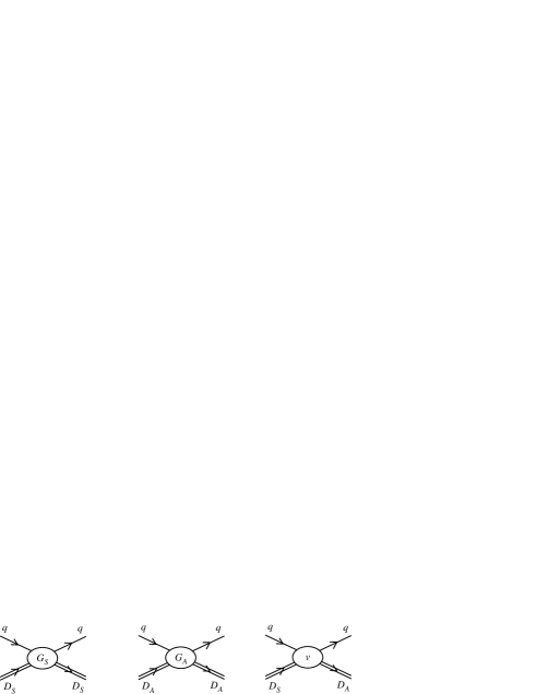
Figure 1: Quark-diquark interactions in various channels.

2.3 Hadronization

Introducing the auxiliary fields for baryons, we can rewrite the Lagrangian as (omit the color indices for brevity)

$${\cal L} = \bar{\chi}(i\hbox to0.0pt{/\hss}\partial-m_{q})\chi\;+\;D^{\dagger}(\partial^{2}+M_{S}^{2})D$$ (6)

$$+ {\vec{D}^{{\dagger}\;\mu}}\left[(\partial^{2}+M_{A}^{2})g_{\mu\nu}-\partial_{\mu}\partial_{\nu}\right]\vec{D}^{\nu}+\bar{\psi}\hat{G}\psi-\bar{B}\hat{G}^{-1}B\,,$$

where $B=(B_{1},B_{2})^{T}$ is a two component auxiliary baryon field, whose components correspond to scalar and axial-vector channels; $B_{1}\sim D\chi$ and $B_{2}\sim\vec{\tau}\cdot\vec{D}_{\mu}\gamma^{\mu}\gamma^{5}\chi$. In Eq. (6) we have introduced matrix notations of $2\times 2$ as

$$\psi = \left(\begin{array}[]{c}D\chi\\ \vec{D}_{\mu}\cdot\vec{\tau}\gamma^{\mu}\gamma^{5}\chi\end{array}\right),\quad\bar{\psi}=\left(\begin{array}[]{cc}\bar{\chi}D^{\dagger},&\bar{\chi}\vec{D}_{\mu}^{\dagger}\cdot\vec{\tau}\gamma^{\mu}\gamma^{5}\end{array}\right),$$ (10)

$$\hat{G} = \left(\begin{array}[]{cc}G_{S}&v\\ v&G_{A}\end{array}\right).$$ (13)

In the hadronization procedure[17, 20, 21], the quark and diquark fields are eliminated and an effective meson-baryon Lagrangian is obtained in the $\mbox{tr}\log$ form as

$${\cal L}=-\bar{B}\hat{G}^{-1}B+i\mbox{Tr}\ln(1-A).$$ (14)

Here the matrix $A$ is defined by

$$A = \left(\begin{array}[]{cc}a_{11}&a_{12}\\ a_{21}&a_{22}\end{array}\right),$$ (17)

$$a_{11} = \Delta^{T}\bar{B}_{1}SB_{1},$$ (18)

$$a_{12} = \Delta^{T}\bar{B}_{2}\tau^{i}\gamma^{\nu}\gamma^{5}SB_{1},$$ (19)

$$a_{21} = (\Delta_{\rho\nu}^{lj})^{T}\bar{B}_{1}S\gamma^{\mu}\gamma^{5}\tau^{j}B_{2},$$ (20)

$$a_{22} = (\Delta_{\rho\nu}^{lj})^{T}\bar{B}_{2}\gamma^{\nu}\gamma^{5}\tau^{i}S\gamma^{\mu}\gamma^{5}\tau^{j}B_{2}.$$ (21)

where $S$, $\Delta$ and $\Delta_{\mu\nu}$ are the propagators of the quark, scalar diquark and axial-vector diquark, respectively.

Expanding the tr log formula in powers of meson and baryon fields, we obtain the self-energies of the nucleons as

$${\cal L}=\bar{B}\left(\begin{array}[]{cc}\Sigma_{S}(p)&0\\ 0&\Sigma_{A}(p)\end{array}\right)B-\frac{1}{|\hat{G}|}\bar{B}\left(\begin{array}[]{cc}G_{A}&-v\\ -v&G_{S}\end{array}\right)B,$$ (26)

where $|\hat{G}|=\mbox{det}\hat{G}=G_{S}G_{A}-v^{2}$. The loop integrals of the self-energies are given by

$$\Sigma_{S}(p) = -iN_{c}\int\frac{d^{4}k}{(2\pi)^{4}}\frac{1}{k^{2}-M_{S}^{2}}\frac{/{p}-/{k}+m_{q}}{(p-k)^{2}-m_{q}^{2}},$$ (27)

$$\Sigma_{A}(p) = -iN_{c}\int\frac{d^{4}k}{(2\pi)^{4}}\frac{k^{\mu}k^{\nu}/M_{A}^{2}-g^{\mu\nu}}{k^{2}-M_{A}^{2}}$$ (28)

$$\;\;\;\times\;\delta_{ij}\gamma_{\nu}\gamma_{5}\tau_{j}\frac{/{p}-/{k}+m_{q}}{(p-k)^{2}-m_{q}^{2}}\tau_{i}\gamma_{\mu}\gamma_{5}.$$

Here $N_{c}$ is the number of colors. In our computation, the divergent integrals of (28) are regularized by the three momentum cutoff scheme[19].

2.4 Diagonalization

We consider nucleon properties in the center of mass system of the nucleon. The self-energies $\Sigma_{S}$ and $\Sigma_{A}$ are then expanded in powers of the four momentum in the rest frame $p_{\mu}=(p_{0},\ \vec{0})$,

$$\Sigma_{S}(p_{0})-\frac{1}{|\hat{G}|}G_{A} = Z_{S}^{-1}(p_{0}\gamma^{0}-a_{S}),$$ (29)

$$\Sigma_{A}(p_{0})-\frac{1}{|\hat{G}|}G_{S} = Z_{A}^{-1}(p_{0}\gamma^{0}-a_{A})\,.$$ (30)

The bare baryon fields $B_{1,2}$ are then renormalized as

$$\left(\begin{array}[]{c}B_{1}\\ B_{2}\end{array}\right)=\left(\begin{array}[]{c}\sqrt{Z_{S}}B_{1}^{\prime}\\ \sqrt{Z_{A}}B_{2}^{\prime}\end{array}\right),$$ (35)

with which the Lagrangian (26) can be written as

$${\cal L}=\bar{B}^{\prime}(p_{0}\gamma^{0}-\hat{M})B^{\prime}\,,$$ (36)

where the mass matrix $\hat{M}$ is given by

$$\hat{M}=\left(\begin{array}[]{cc}a_{S}&-\sqrt{Z_{S}Z_{A}}\frac{v}{|\hat{G}|}\\ -\sqrt{Z_{S}Z_{A}}\frac{v}{|\hat{G}|}&a_{A}\end{array}\right).$$ (39)

Now the mass matrix can be diagonalized through a unitary transformation:

$$B^{\prime} = U^{\dagger}N\,,\;\;\;U\hat{M}U^{\dagger}=\left(\begin{array}[]{cc}M_{1}&0\\ 0&M_{2}\end{array}\right).$$ (42)

One finds

$${\cal L}=\bar{N_{1}}(p_{0}\gamma^{0}-M_{1})N_{1}+\bar{N_{2}}(p_{0}\gamma^{0}-M_{2})N_{2},$$ (43)

where the physical eigenvalues $M_{1,2}$ and eigenvectors $N=(N_{1},\ N_{2})^{T}$ are obtained as

$$M_{1,2} = \frac{1}{2}\left[a_{S}+a_{A}\pm\sqrt{(a_{S}-a_{A})^{2}+4Z_{S}Z_{A}\left(\frac{v}{|\hat{G}|}\right)^{2}}\right]\,,$$ (44)

$$N_{1} = \cos\phi B_{1}^{\prime}+\sin\phi B_{2}^{\prime}\,,\;\;N_{2}=-\sin\phi B_{1}^{\prime}+\cos\phi B_{2}^{\prime}\,,$$ (45)

and the mixing angle $\phi$ is given by

$$\tan 2\phi=\frac{2\sqrt{Z_{S}Z_{A}}v}{(a_{A}-a_{S})|\hat{G}|}$$ (46)

Eq. (44) should be read as a self-consistent equation where the quantities on the right hand side are functions of $M_{1,2}$. The equations are then equivalent to the Schrodinger equation for the quark-diquark system interacting through the delta function type interaction with suitable cutoff.

3 Results and discussions

First let us fix model parameters. The constituent masses of $ud$ quarks $m_{q}$ and the three momentum cutoff $\Lambda$ are fixed in such a way that they reproduce meson properties in the NJL model[22, 23]. The masses of the diquarks may be calculated in the NJL model [22, 24], but here we treat them as parameters. In this way we employ $m_{q}$=390 MeV, $\Lambda$=600 MeV, $M_{S}$=650 MeV and $M_{A}$=1050 MeV. The mass difference $M_{A}-M_{S}$ may be related to that of the nucleon and delta. In the quark-diquark model, the delta is described as a bound state of an axial-vector diquark and a quark, while the nucleon is expected to be dominated by the scalar diquark component. Hence, we expect that the $N\Delta$ mass difference is roughly given by the mass difference of the axial and scalar diquarks. This qualitatively justifies the mass difference $M_{A}-M_{S}\sim 400$ MeV that we adopt.

The masses of the two nucleon states may be studied as functions of the coupling constants, $G_{S}$, $G_{A}$ and $v$. For instance, we can fix the diagonal strengths $G_{S}$, $G_{A}$, and vary the off-diagonal strength $v$ to see the effect of the mixing. In this procedure, however, the binding energy of the quark-diquark system also changes which significantly affects the sizes of the nucleon and Roper. For some coupling constants, the nucleon becomes unphysically too large. In order to overcome this difficulty, we fix the quark-diquark binding energies to be always 50 MeV for both scalar and axial-vector diquark nucleons as $v$ is varied. This can be realized by choosing $G_{S}$ and $G_{A}$ appropriately, and the resulting bound states produces nucleon size reasonably [17, 18]. The results for the masses of the nucleon and Roper are shown in Figure 2. We find that $M_{1}=$ 0.94 GeV, $M_{2}$=1.44 GeV and $\phi$ =18 degree at $v\sim$ 22 GeV^-1. Due to the fixed binding energy, we find that the plot looks very much the same as the one familiar in a two level problem of the quantum mechanics.

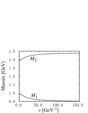
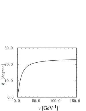
Figure 2: The masses $M_{1,2}$ as functions of the mixing strength $v$ (left) and the mixing angle $\phi$ (right). The coupling constants $G_{S}$ and $G_{A}$ are determined such that the binding energies of the quark-diquark system takes 50 MeV.

The present identification of the Roper resonance is very much different from the conventional picture; in the quark model, it is described as an excited state of $2\hbar\omega$ with $(n,l)=(1,0)$, where $(n,l)$ are the principle and angular momentum quantum numbers of the harmonic oscillator wave function. The excitation energy of such a state is as high as $2\hbar\omega\sim 1$ GeV for the oscillator parameter $\omega\sim 0.5$ GeV, and many mechanisms have been proposed to lower the energy [25]. In the present picture the two nucleons are described as quark-diquark bound states, but with different diquarks of scalar and axial-vector ones.

In the quark model, these diquarks correspond to the $\rho$ and $\lambda$ type two-quark states, which in the limit of SU(6) spin-flavor symmetry can not be independent degrees of freedom due to the Pauli principle when constructing the nucleon state of $J^{P}=1/2^{+}$. In the present case, if the strong correlation between the quarks is at work, the two quark states violate the SU(6) symmetry, and they can be independent. In the harmonic oscillator basis, the two quarks of the diquarks are in the ground state but with being correlated. The energy difference is therefore supplied not by the difference in the single particle energies of nodal excitation, but rather by the residual correlation between the quarks. This is the mechanism that makes the mass of the Roper significantly lower than the conventional radial exitation.

It is also interesting to look at the spatial structure of the nucleon and Roper when they are given as superpositions of the two diquark components (45). Intrinsically, the scalar diquark is a tightly bound state of two quarks while the axial-vector looser. Therefore, the wave function of the scalar diquark nucleon $B_{1}^{\prime}$ is more compact than the axial-vector diquark nucleon $B_{2}^{\prime}$. If the wave functions of $B_{1}^{\prime}$ and $B_{2}^{\prime}$ are coherently added with a constructive phase for the nucleon ($N_{1}$), then for the Roper ($N_{2}$) they are added destructively. Hence, we expect qualitatively different structure in the wave function for the nucleon and Roper as shown in Figure 3. It is interesting that the wave function of the Roper has a nodal structure as a consequence of the two components of $B_{1}^{\prime}$ and $B_{2}^{\prime}$ just as in the nodal excitation in the naive quark model.

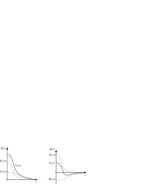
Figure 3: A qualitative sketch for quark distributions for the nucleon and Roper.

4 Summary

In this report, we have discussed the nucleon and Roper resonance in the chiral quark-diquark model. It was shown that the two states appear as the ground state in orbital configuration but with different spin and isospin structure. In the SU(6) quark model, one of these states is forbidden due to the Pauli exclusion principle, which, however, can survive as an independent degree due to diquark correlations.

In a sample calculation, we have reproduced the masses of the nucleon and Roper by employing suitable parameters. This encourages us to further investigate this picture for the nucleon and Roper. As a straightforward application, the present model should be tested for electromagnetic properties of the nucleon and the Roper. For the nucleon, we expect that the inclusion of the axial-vector diquark improves the small magnetic moments and the axial-vector coupling constants when only scalar diquark is considered.

The description of the nucleon and Roper as the ground state with different spin-isospin structure reminds us the Weinberg’s idea that they are regarded as chiral partners which belong to the same chiral multiplet. In this way we may be able to explain the masses and the coupling relations among the nucleons and the Roper. Relation with the chiral symmetry is particularly interesting and will be studied when written the diquark fields explicitly by the quark fields. Some consequences of such descriptions will be reported elsewhere [14].

References

- [1] N. Isgur and G. Karl, Phys. Rev. D 18, 4187 (1978).
- [2] N. Isgur and G. Karl, Phys. Rev. D 20, 1191 (1979).
- [3] M. Takayama, H. Toki and A. Hosaka, Prog. Theor. Phys. 101, 1271 (1999).
- [4] G. E. Brown, J. W. Durso and M. B. Johnson, Nucl. Phys. A 397 447 (1983).
- [5] T. Hatsuda, Nucl. Phys. A 458 583 (1986).
- [6] J. D. Breit and C. R. Nappi, Phys. Rev. Lett. 53 889 (1984).
- [7] A. Hayashi, G. Eckart, G. Holzwarth and H. Walliser, Phys. Lett. B 147 5 (1984).
- [8] I. Zahed, U. G. Meissner and U. B. Kaulfuss, Nucl. Phys. A 426, 525 (1984).
- [9] M. P. Mattis and M. E. Peskin, Phys. Rev. D 32 58 (1985).
- [10] A. Hosaka and H. Toki, Z. Phys. A 330, 111 (1988).
- [11] S. Weinberg, Phys. Rev. 177, 2604 (1969).
- [12] S. R. Beane and U. van Kolck, J. Phys. G 31, 921 (2005) [arXiv:nucl-th/0212039].
- [13] S. R. Beane and M. J. Savage, Phys. Lett. B 556, 142 (2003) [arXiv:hep-ph/0212106].
- [14] K. Nagata, A. Hosaka and V. Dmitrasinovic, In preparation.
- [15] R. Jaffe, Phys. Rev. D 72, 074508 (2005) [arXiv:hep-ph/0507149].
- [16] R. L. Jaffe, Phys. Rept. 409, 1 (2005) [Nucl. Phys. Proc. Suppl. 142, 343 (2005)] [arXiv:hep-ph/0409065].
- [17] L. J. Abu-Raddad, A. Hosaka, D. Ebert and H. Toki, Phys. Rev. C 66 025206 (2002).
- [18] K. Nagata and A. Hosaka, Prog. Theor. Phys. 111, 857 (2004).
- [19] K. Nagata, A. Hosaka and L. J. Abu-Raddad, [arXiv:hep-ph/0408312].
- [20] R. T. Cahill, Austral. J. Phys. 42, 171 (1989).
- [21] H. Reinhardt, Phys. Lett. B 244, 316 (1990).
- [22] U. Vogl and W. Weise, Prog. Part. Nucl. Phys. 27 195 (1991).
- [23] T. Hatsuda and T. Kunihiro Phys. Rept, 247, 221 (1994).
- [24] R. T. Cahill, C. D. Roberts and J. Praschifka, Phys. Rev. D36, 2804 (1987).
- [25] L. Y. Glozman and D. O. Riska, Phys. Rept. 268, 263 (1996).