A study on the radiative dileptonic decays $B^{0}(B_{s})\to\gamma\ell^{+}\ell^{-}$

Abstract

We study the rare radiative dileptonic decays $B^{0}(B_{s})\to\gamma\ell^{+}\ell^{-}$ ($\ell=e,\mu$) in the standard model. By using the $B$ meson wave function constrained by non-leptonic decays, the branching ratios turn out to be of the order of $10^{-9}$ for $B_{s}\to\gamma\mu^{+}\mu^{-}$, $\gamma e^{+}e^{-}$ and $10^{-10}$ for $B^{0}\to\gamma\mu^{+}\mu^{-}$, $\gamma e^{+}e^{-}$. Based on the study, these decays are accessible at the near future LHC-b experiment, which are useful to determine the $B(B_{s})$ wave function.

1 Introduction

The radiative and leptonic B decays have been the subject of many theoretical studies in the framework of the Standard Model (SM) and the search of new physics. These processes play an important role in determining the parameters of the SM and some hadronic parameters in QCD, such as the Cabibbo-Kobayashi-Maskawa (CKM) matrix elements, the meson decay constant $f_{B}$, and $f_{B_{s}}$. Especially, the radiative leptonic decays can provide information on heavy meson wave functions [1]. Being rare decays in SM, they are also very sensitive to any new physics contributions.

Due to the GIM mechanism [2], there is absence of flavor changing neutral current transition at the tree level, thus, the pure leptonic processes $B^{0}(B_{s})\to\ell^{+}\ell^{-}$ ($\ell=e,\mu$) can only occur via penguin and box diagrams. In addition, rare decays of heavy pseudoscalar meson into light lepton pairs are helicity suppressed. Some of the branching ratios are very small, for instance [3] $B_{r}(B_{s}\to\mu^{+}\mu^{-})=2\times 10^{-9}$ and $B_{r}(B_{s}\to e^{+}e^{-})=4\times 10^{-14}$, so it is difficult for us to extract the $B_{s}$ meson decay constant information from these processes. For $B^{0}$ meson, the situation is even worse due to the smaller CKM matrix elements. Although the process $B_{s}\to\tau^{+}\tau^{-}$ is free from this helicity suppression mechanism, the branching ratio turns out to be around $8\times 10^{-7}$ in the SM [4], which is much larger than the branching ratios of $B_{s}\to\mu^{+}\mu^{-}$, $B_{s}\to e^{+}e^{-}$, it is still hard to be detected at B-factory where the efficiency is not better than $10^{-2}$.

Because of massless neutrino, the decay $B^{0}(B_{s})\to\nu\bar{\nu}$ is helicity forbidden. While, if an additional real photon is emitted, the forbidden situation will change [5, 6]. Similarly the helicity suppression in the pure leptonic B decays $B^{0}(B_{s})\to\ell^{+}\ell^{-}$ will be cured in the radiative decay $B^{0}(B_{s})\to\gamma\ell^{+}\ell^{-}$. This is already shown in the simple constituent quark model calculation [7], light cone QCD [8]. In this paper, we employ the $B$ meson distribution amplitude derived from non-leptonic B decays to analyze these processes again.

We organize our paper as follows: In Sec.2, the relevant effective Hamiltonian will be given in the SM. In Sec.3, the wave function of $B$ meson will be used to calculate these processes, and later some comparison will be given. Finally, Sec.4 includes a brief conclusion.

2 Effective Hamiltonian

Let us start with the quark level processes $b\to q\ell^{+}\ell^{-}$, with $q=s$ or $d$ quark, $\ell=e$ or $\mu$. The leading order Feynman diagrams are shown in Fig.1. It is easy to see that the magnetic penguin, $Z$ penguin and box diagrams contribute to these processes. They are subject to QCD corrections which can be obtained by connecting the quark lines by gluon lines. The effective Hamiltonian in SM for them is [9]:

$${\cal H}_{eff}=\frac{\alpha{G_{F}}}{\sqrt{2}\pi}V_{tb}V^{*}_{tq}\left\{\left[\frac{2{C_{7}}{m_{b}}}{q^{2}}\bar{q}P_{R}(\not\!p\gamma^{\mu}-\gamma^{\mu}\not\!p)b+C^{eff}_{9}\bar{q}\gamma^{\mu}{P_{L}}b\right]\bar{l}\gamma_{\mu}{l}+C_{10}(\bar{q}\gamma^{\mu}{P_{L}}b)~{}\bar{l}\gamma_{\mu}\gamma_{5}{l}\right\},$$ (1)

where $P_{L}=(1-\gamma_{5})/{2}$, $P_{R}=(1+\gamma_{5})/{2}$, $q^{2}=(P_{+}+P_{-})^{2}$, with $P_{+}$ and $P_{-}$ are the momenta of lepton pair. $C_{7}$, $C^{eff}_{9}$, and $C_{10}$ are the $QCD$ corrected Wilson coefficients, whose specific forms are given in Ref.[10].

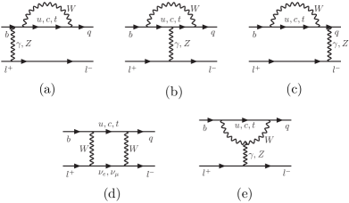
Figure 1: Leading-order diagrams for $b\to q\ell^{+}\ell^{-}$ transition in SM.

If an additional photon line is attached to any of the charged lines in Fig.1, we will have the radiative leptonic decays $b\to q\gamma\ell^{+}\ell^{-}$. In fact, there are two kinds of diagrams: photon connecting to the internal line of Fig.1, and photon connecting to the external line of Fig.1. For the first kind of diagrams, because of the effective operators are dimension-8 instead of dimension-6, there will be a suppression factor of $m_{b}^{2}/m_{W}^{2}$ in the Wilson coefficients compared with the ones for $b\to q\ell^{+}\ell^{-}$. Therefore we will only consider the second category of diagrams. In this case, we only have dimension 6 operators with an additional photon from any of the fermion lines, which are shown in Fig.2.

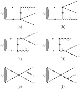
Figure 2: Feynman diagrams for $B_{q}\to\gamma{\ell^{+}}{\ell^{-}}$ in the SM (black dots are dimension 6 operators).

First, let us study the Fig.2(e) and (f) with photon attached to external lepton lines. Being a pseudoscalar meson, $B$ meson can only decay through axial current, so

$$<0|\bar{q}\sigma^{\mu\nu}{P_{R}}b|B>=0.$$ (2)

That is to say, in diagrams (e) and (f), the magnetic penguin operator $O_{7}$ ’s contribution vanishes. Our numerical calculation shows that: the contribution from other operators for these two diagrams are also very small, we can neglect their contribution safely. Similarly for Fig.2 (c) and (d), We find numerically they are also negligibly small comparing with Fig.2 (a) and (b). Thus the main contribution to $B^{0}(B_{s})\to\gamma{\ell^{+}\ell^{-}}$ comes from the Fig.2 (a) and (b), which agrees with the constituent quark model calculation [7].

Let us analyze the diagrams (a) and (b) in Fig.2, with photon emitted from the external quark lines $b$ or $q$. After calculation, we get the amplitude:

$${\cal A} = \frac{e}{2}\bar{q}\left[\not\!\varepsilon\frac{\not\!{k}-\not\!{p_{2}}+m_{q}}{p_{2}.k}\gamma^{\mu}{P_{L}}+\gamma^{\mu}{P_{L}}\frac{\not\!{p_{1}}-\not\!{k}+m_{b}}{p_{1}.k}\not\!\varepsilon\right]b.\left[C^{eff}_{9}\bar{l^{-}}\gamma_{\mu}{l^{+}}+C_{10}\bar{l^{-}}\gamma_{\mu}\gamma_{5}{l^{+}}\right]$$

$$+ \frac{e}{2}\frac{C_{7}m_{b}}{q^{2}}\bar{q}\left[{P_{R}}(\not\!{q}\gamma^{\mu}-\gamma^{\mu}\not\!{q})\not\!\frac{\not\!{p_{1}}-\not\!{k}+m_{b}}{p_{1}.k}\not\!\varepsilon+\not\!\varepsilon\frac{\not\!{k}-\not\!{p_{2}}+m_{q}}{p_{2}.k}(\not\!{q}\gamma^{\mu}-\gamma^{\mu}\not\!{q}){P_{R}}\right]b.[\bar{l^{-}}\gamma_{\mu}{l^{+}}],$$

where $p_{1}$, $p_{2}$ and $k$ are the momenta of $b$, $q$ quark and photon, respectively.

3 Model calculations

To simplify the decay amplitude in eq.(2), we have to utilize the B meson wave function, which is not known from the first principal. Fortunately, many studies on non-leptonic B [11, 12] and $B_{s}$ decays [13] have constrained the wave function strictly:

$$\Phi_{B}=\frac{1}{\sqrt{6}}(\not\!p_{B}+m_{B})\gamma_{5}~{}\phi_{B}({x}),$$ (4)

where the distribution amplitude $\phi_{B}$ can be expressed as [14]:

$$\phi_{B}(x)=N_{B}x^{2}(1-x)^{2}\exp\left[-\frac{M_{B}^{2}\ x^{2}}{2\omega_{b}^{2}}\right].$$ (5)

It satisfies the normalization relation:

$$\int_{0}^{1}\phi_{B}(x)dx=\frac{f_{B}}{2\sqrt{2N_{c}}}\;,$$ (6)

with $f_{B}$ is the $B$ meson decay constant.

From definition of the wave function, we have $p_{b}=(1-x)P_{B}$, $p_{q}=xP_{B}$, and the decay amplitude (2) is then:

$$A=C\left[iC_{1}\epsilon_{\alpha\beta\mu\nu}P^{\alpha}_{B}\varepsilon^{\beta}{k^{\nu}}+C_{2}(k_{\mu}\varepsilon_{\nu}-\varepsilon_{\mu}{k}_{\nu})P^{\nu}_{B_{q}}\right]\left[(C^{eff}_{9}-\frac{2C_{7}M_{B}^{2}}{q^{2}})\bar{l^{-}}\gamma^{\mu}{l^{+}}+C_{10}\bar{l^{-}}\gamma^{\mu}\gamma_{5}{l^{+}}\right]$$ (7)

with $C=\frac{e\alpha{G_{F}}}{\sqrt{12}\pi}|V_{tb}V^{*}_{tq}|,$ and

$$C_{1}=\left(\int_{0}^{1}\frac{\phi_{B}(x)}{1-x}dx+\int_{0}^{1}\frac{\phi_{B}(x)}{x}dx\right),$$

$$C_{2}=\left(\int_{0}^{1}\frac{\phi_{B}(x)}{1-x}dx-\int_{0}^{1}\frac{\phi_{B}(x)}{x}dx\right).$$ (8)

After squaring the amplitude, and then performing the phase space integration over one of the two Dalitz variables, we get the differential decay width versus the photon energy $E_{\gamma}$,

$$\frac{d\Gamma}{dE_{\gamma}}=\frac{2\alpha^{3}{G^{2}_{F}}}{12^{2}\pi^{4}}|V_{tb}V^{*}_{tq}|^{2}(C^{2}_{1}+C^{2}_{2})(M_{B_{q}}-2E_{\gamma})E_{\gamma}\left[\left(C^{eff}_{9}-\frac{2M_{B_{q}}C_{7}}{M_{B_{q}}-2E_{\gamma}}\right)^{2}+C^{2}_{10}\right].$$ (9)

Table 1: Comparison of branching ratios with other model calculations

	Our Results	Quark Model[7]	light cone [8]
$\mathbf{BR}(B_{s}\to\gamma\mu^{+}\mu^{-})$	$1.7^{-0.46}_{+0.98}\times 10^{-9}$	$4.6\times 10^{-9}$	$1.9\times 10^{-9}$
$\mathbf{BR}(B_{s}\to\gamma{e^{+}}{e^{-}})$	$1.9^{-0.52}_{+1.21}\times 10^{-9}$	$6.2\times 10^{-9}$	$2.35\times 10^{-9}$
$\mathbf{BR}(B^{0}\to\gamma\mu^{+}\mu^{-})$	$0.65^{-0.23}_{+0.36}\times 10^{-10}$	$6.2\times 10^{-10}$	$1.2\times 10^{-10}$
$\mathbf{BR}(B^{0}\to\gamma{e^{+}}{e^{-}})$	$0.83^{-0.21}_{+0.48}\times 10^{-10}$	$8.2\times 10^{-10}$	$1.5\times 10^{-10}$

In numerical calculations, we use the following parameters [15]:

$$\alpha=\frac{1}{137},~{}G_{F}=1.66\times 10^{-5}\mathrm{GeV}^{-2},\omega_{b}=0.4,~{}f_{B}=0.19~{}\mathrm{GeV},$$

$$\omega_{b_{s}}=0.5,~{}f_{Bs}=0.24~{}\mathrm{GeV},|V_{tb}|=0.999,~{}~{}|V_{td}|=0.007,~{}~{}|V_{ts}|=0.041,$$

$$M_{B^{0}}=5.28~{}\mathrm{GeV},~{}M_{B_{s}}=5.37~{}\mathrm{GeV},~{}\tau_{B}=1.54\times 10^{-12}s,~{}\tau_{B_{s}}=1.46\times 10^{-12}s.$$ (10)

After integration of phase space, we get the decay branching ratios shown in Table 1 together with numbers from other models. The input parameters $\alpha$, $f_{B}$ and CKM factors will only give an overall factor to the uncertainty of branching ratios, which can be obtained easily, thus we do not show them. The uncertainty shown in the Table 1 comes from the heavy meson wave function, by varying the parameter $\omega_{b}=0.4\pm 0.1$, and $\omega_{b_{s}}=0.5\pm 0.1$. From this strong sensitivity, we know that the radiative decays can provide information or constraints on the $B(B_{s})$ meson wave functions. Surely more uncertainty can come from the next-to-leading order contribution which is difficult to estimate. From the table, we can see that our results are similar to the results from the light cone sum rule [8], but smaller than the constituent quark model [7]. If we interpret the second term of eq.(8) as the inverse of the constituent quark mass, we will find that it corresponds to $m_{d}\simeq 473$MeV which is larger than that used in ref.[7]. The simple picture of constituent quark model gives a larger result due to the smaller constituent quark mass. But the much smaller result for $B^{0}$ decays, which is even smaller than the light come sum rule one [8], is due to the smaller CKM factor $|V_{td}|$ used here.

Figure 3: Differential decay rate for $B_{s}(B^{0})\to\gamma{\ell^{+}}{\ell^{-}}$ versus the photon energy ${E_{\gamma}}$.

The differential decay width as a function of $E_{\gamma}$ is displayed in Fig.3. Most of the contribution is with an energetic photon which is easier for the experiment. One may expect that through the mechanism of vector meson dominance [16], long distance effects also contribute to the process $B^{0}(B_{s})\to\gamma\ell^{+}\ell^{-}$ ($\ell=e,\mu$). Some detailed calculation [17] indicates that: the long distance contributions are significant in the resonance region. It is probably not easy to derive short distance information from the dominant long distance contributions by total decay width. Therefore, the photon energy spectrum shown in Fig.3 will be helpful to distinguish those contributions.

4 summary

We calculate the rare decays $B^{0}(B_{s})\to\gamma\ell^{+}\ell^{-}$ in SM. Utilizing the $B$ ($B_{s}$) meson wave functions constrained by non-leptonic decays, the branching ratio is predicted at the order of $10^{-9}$ for $B_{s}\to\gamma\ell^{+}\ell^{-}$ and $10^{-10}$ for $B^{0}\to\gamma\ell^{+}\ell^{-}$. There are possibilities to detect them in the LHC-b experiments, which could provide information on the $B$ ($B_{s}$) meson wave function or new physics signal [18].

References

• [1] G.Β Burdman, T.Β Goldman and D.Β Wyler, Phys. Rev. D51, 111 (1995);
Y.-Y. Charng, H.n. Li, Phys. Rev. D 72, 014003, (2005).
• [2] S.L. Glashow, J. Iliopoulos and L. Malani, Phys. Rev. D 2, 1285-1292, (1970).
• [3] B.A. Campbell and P.J. O’Donnell, Phys. Rev. D 25 (1982) 1989;
A. Ali, B decays, ed. S. Stone (World Scientific, Singapore) p.67.
• [4] G. Buchalla and A.J. Buras, Nucl. Phys. B 400 (1993) 225.
• [5] C.-D. LΓΌ, D.-X. zhang, Phys. lett. B 381 (1996) 348.
• [6] Jun-Xiao Chen, Zhao-Yu Hou and Cai-Dian-LΓΌ, High Energy Phys. $\&$ Nucl. Phys, Vol. 30-4, 289-293 (2006).
• [7] G. Eilam, C.-D. LΓΌ and D.-X. Zhang, Phys. Lett. B 391 (1997) 461.
• [8] T.M. Aliev, A. Ozpineci, M. Savci, Phys. Rev. D 55, 7059-7066, (1997).
• [9] R. Grigjanis et al., Phys. Lett. B 213 (1998) 247;
W.S. Hou and R.S. Willey, Phys. Lett. B 202 (1988) 591;
B. Grinstein, M.J. Savage and M.B. Wise, Nucl. Phys. B 319 (1989) 271;
G. Cella, G. Ricciardi and A. Vicere, Phys. Lett. B 258 (1991) 212;
A.J. Buras and M. MΓΌnz, Phys. Rev. D 52 (1995) 186.
• [10] N. Cabibbo and L. Maiani, Phys. Lett. B 79 (1979) 109;
M. Misiak, Nucl. Phys. B 393 (1993) 23-45; B 439 (1995) 461(E).
• [11] C.-D.Β LΓΌ, K.Β Ukai and M.-Z.Β Yang, Phys. Rev. D 63, 074009 (2001);
Y.-Y.Β Keum, H.-n.Β Li and A.I.Β Sanda, Phys. Lett. B 504, 6 (2001);
Phys. Rev. D 63, 054008 (2001);
H.-n. Li, Phys. Rev. D 64, 014019 (2001); S.Β Mishima, Phys. Lett. B 521, 252 (2001);
C.-H.Β Chen, Y.-Y.Β Keum, and H.-n.Β Li, Phys. Rev. D64, 112002 (2001); Phys. Rev. D 66, 054013 (2002).
• [12] C.D.Β LΓΌ, Eur. Phys. J. C 24, 121 (2002); Phys. Rev. D 68, 097502 (2003);
Y.-Y.Β Keum and A.I.Β Sanda, Phys. Rev. D 67, 054009(2003);
Y.-Y.Β Keum, et al., Phys. Rev. D 69, 094018 (2004);
J.Β Zhu, Y.L.Β Shen and C.D.Β LΓΌ, Phys. Rev. D 72, 054015 (2005); Eur. Phys. J. C41, 311 (2005);
Y.Β Li and C.D.Β LΓΌ, J. Phys. G 29, 2115 (2003); and Phys. Rev. D73, 014024 (2006);
Y.Β Li, C.D.Β LΓΌ, and Z.J.Β Xiao, J. Phys. G 31, 273 (2005);
C.D.Β LΓΌ, M.Β Matsumori, A.I.Β Sanda, and M.Z.Β Yang, Phys. Rev. D 72, 094005 (2005).
• [13] Y.Β Li, C.D.Β LΓΌ, Z.J.Β Xiao, and X.Q.Β Yu, Phys. Rev. D 70, 034009 (2004);
J.Β Zhu, Y.L.Β Shen and C.D.Β LΓΌ, J. Phys. G 32, 101 (2006);
Y.Β Li and C.D.Β LΓΌ, Commun. Theor. Phys. 44, 659 (2005);
X.QΒ Yu, Y.Β Li and C.D.Β LΓΌ, Phys. Rev. D 71, 074026 (2005); Phys. Rev. D 73, 017501, (2006).
• [14] C.-D.Β LΓΌ and M.-Z.Β Yang, Eur. Phys. J. C 28, 515-523 (2003).
• [15] Particle Data Group, S. Eidelman, et al., Phys. Lett. B 592,1 (2004);
LI H.-N, B. Melic, Eur. Phys. J. C 11 (1999) 695;
HUANG Tao, WU X.-G, Phys. Rev. D 71 (2005) 034018.
• [16] N.G. Deshpande, J. Trampetic and K. Panose, Phys. Rev. D 39 (1989) 1461;
N. Paver and Riazuddin, Phys. Rev. D 45 (1992) 978;
P.J. O’Donnell and H.K.K. Tung, Phys. Rev. D 43 (1991) 2067;
C.S. Lim, T. Morozumi and A.I. Sanda, Phys. Lett. B 218 (1989) 343.
• [17] C.-D. LΓΌ and D.-X. Zhang, Phys, Lett. B 397 (1997) 279-282.
• [18] T.M. Aliev, A. Ozpineci, M. Savci, Phys. Lett. B 520, 69-77, 2001; Eur. Phys. J. C 27, 405-410, (2003);
G. Erkol, G. Turan, Acta Phys. Polon. B 33, 1285-1311, (2002)
S. R. Choudhury, N. Gaur, N. Mahajan, Phys. Rev. D 66, 054003, 2002;
U.O. Yilmaz, B.B. Sirvanli, G. Turan, Eur. Phys. J. C 30, 197-205, (2003);
S. R. Choudhury, et al., hep-ph/0504193;
A.K. Alok, S.U. Sankar, hep-ph/0611215.