Limits on the Electromagnetic and Weak Dipole Moments of the Tau-Lepton in $E_{6}$ Superstring Models

Abstract

We obtain limits on the electromagnetic and weak dipole moments of the tau-lepton in the framework of a Left-Right symmetric model (LRSM) and a class of $E_{6}$ inspired models with an additional neutral vector boson $Z_{\theta}$. Using as an input the data obtained by the L3 and OPAL Collaborations for the reaction $e^{+}e^{-}\to\tau^{+}\tau^{-}\gamma$, we get a stringent limit on the LRSM mixing angle $\phi$, $-1.66\times 10^{-3}<\phi<1.22\times 10^{-3}$, which in turn induces bounds on the tau weak dipole moments which are consistent with the bounds obtained recently by the DELPHI and ALEPH Collaborations from the reaction $e^{+}e^{-}\to\tau^{+}\tau^{-}$. We also get similar bounds for the weak dipole moments of the tau lepton in the framework of $E_{6}$ superstring models.

I Introduction

The production of tau-lepton pairs in high energy $e^{+}e^{-}$ collisions has been used to set bounds on its electromagnetic and weak dipole moments Lohmann ; L3D ; DELPHI ; ALEPH . In the Standard Model (SM) S.L.Glashow ; S.Weinberg ; A.Salam , the $\tau$ anomalous magnetic moment (MM) $a_{\tau}=(g_{\tau}-2)/2$ is predicted to be $(a_{\tau})_{SM}=0.0011773(3)$ Samuel ; Hamzeh and the respective electric dipole moment (EDM) $d_{\tau}$ is generated by the GIM mechanism only at very high order in the coupling constant Barr . Similarly, the weak MM and EDM are induced in the SM at the loop level giving $a^{W}_{\tau}=-(2.10+0.61i)\times 10^{-6}$ Bernabeu ; Bernabeu1 and $d^{W}_{\tau}\leq 8\times 10^{-34}e$cm Bernreuther ; Booth . Since the current bounds on these dipole moments Lohmann ; L3D ; DELPHI ; ALEPH are well above the SM predictions, it has been pointed out that these quantities are excellent candidates to look for physics beyond the SM Bernabeu ; Bernabeu1 ; Bernreuther ; Booth ; Gonzalez-Garcia ; Poulose ; Huang ; Escribano ; Grifols ; Taylor ; G.Gonzalez ; G.Gonzalez1 ; G.Gonzalez2 . The couplings of the photon and $Z$ gauge boson to charged leptons may be parametrized in the following form

$$\Gamma^{\alpha}_{V}=eF_{1}(q^{2})\gamma^{\alpha}+\frac{ie}{2m_{l}}F_{2}(q^{2})\sigma^{\alpha\mu}q_{\mu}+eF_{3}(q^{2})\gamma_{5}\sigma^{\alpha\mu}q_{\mu},$$ (1)

where $V=\gamma,Z$, $m_{l}$ is the lepton mass and $q=p^{\prime}-p$ is the momentum transfer. The $q^{2}$-dependent form-factors $F_{i}(q^{2})$ have familiar interpretations for $q^{2}=0$: $F_{1}(0)\equiv Q_{l}$ is the electric charge; $F_{2}(0)\equiv a_{l}$; and $F_{3}\equiv d_{l}/Q_{l}$. The weak dipole moments are defined in a similar way: $F^{Z}_{2}(q^{2}=m^{2}_{Z})=a^{W}_{\tau}$ and $F^{Z}_{3}(q^{2}=m^{2}_{Z})=d^{W}_{\tau}/e$. The measurement of $a^{W}_{\tau}$ and $d^{W}_{\tau}$ has been done in the $Z_{1}\to\tau^{+}\tau^{-}$ decay mode at LEP. The latest bounds obtained for the electromagnetic and weak dipole moments from the DELPHI and ALEPH collaborations at the 95$\%$ C.L. are: $-0.052<a_{\tau}<0.013$, $-0.22<d_{\tau}(10^{-16}\hskip 2.84526pte\mbox{cm})<0.45$ and $a^{W}_{\tau}<1.1\times 10^{-3}$, $d^{W}_{\tau}<0.50\times 10^{-17}e\mbox{cm}$ DELPHI ; ALEPH .

The first limits on the MM and EDM of the $\tau$ lepton were obtained by Grifols and Méndez using L3 data Grifols : $a_{\gamma}\leq 0.11$ and $d_{\gamma}\leq 6\times 10^{-16}e$cm. Escribano and Massó Escribano later on used electroweak precision measurements to get $d_{\tau}\leq 1.1\times 10^{-17}e$cm and $-0.004\leq a_{\tau}\leq 0.006$ at the $2\sigma$ confidence level. There is an extensive theoretical work done in models beyond the SM that contribute to EDM of charged leptons. In Ref. Iltan the EDM of charged leptons are studied assuming that they have Gaussian profiles in extra dimensions. In Dutta the lepton EDM has been analyzed in the framework of the seesaw model. The electric dipole moments of the leptons in the version III of the 2HDM are considered in Iltan1 . The work Iltan2 was related to the lepton EDM in the framework of the SM with the inclusion of non-commutative geometry. Furthermore, the effects of non-universal extra dimensions on the EDM of fermions in the two Higgs doublet model have been estimated in Ref. Iltan3 .

The existence of a heavy neutral ($Z^{\prime}$) vector boson is a feature of many extensions of the standard model. In particular, one (or more) additional $U(1)^{\prime}$ gauge factor provides one of the simplest extensions of the SM. Additional $Z^{\prime}$ gauge bosons appear in Grand Unified Theories (GUT’s) Robinett ; Robinett1 ; Robinett2 ; Langacker2 , Superstring Theories Green ; Green1 ; Gross ; Witten ; Witten1 ; Candelas ; Dine ; Ellis ; Breit ; Candelas1 ; Cecotti , Left-Right Symmetric Models (LRSM) Mohapatra ; G.Senjanovic ; Shrock ; G.Senjanovic1 and in other models such as models of composite gauge bosons Schrempp ; Baur ; Kuroda . The largest set of extended gauge theories are those which are based on GUT’s. Popular examples are the groups $SO(10)$ and $E_{6}$. Generically, additional $Z$-bosons originating from $E_{6}$ grand unified theories are conveniently labeled in terms of the chain: $E_{6}\to SO(10)\times U(1)_{\psi}\to SU(5)\times U(1)_{\chi}\times U(1)_{\psi}\to SM\times U(1)_{\theta_{E_{6}}}$ where $U(1)_{\theta_{E_{6}}}$ remains unbroken at low energies. Detailed discussions on GUTS can be found in the literature Robinett ; Robinett1 ; Robinett2 ; Langacker2 ; Green ; Green1 ; Gross ; Witten ; Witten1 ; Candelas ; Dine ; Ellis ; Breit ; Candelas1 ; Cecotti .

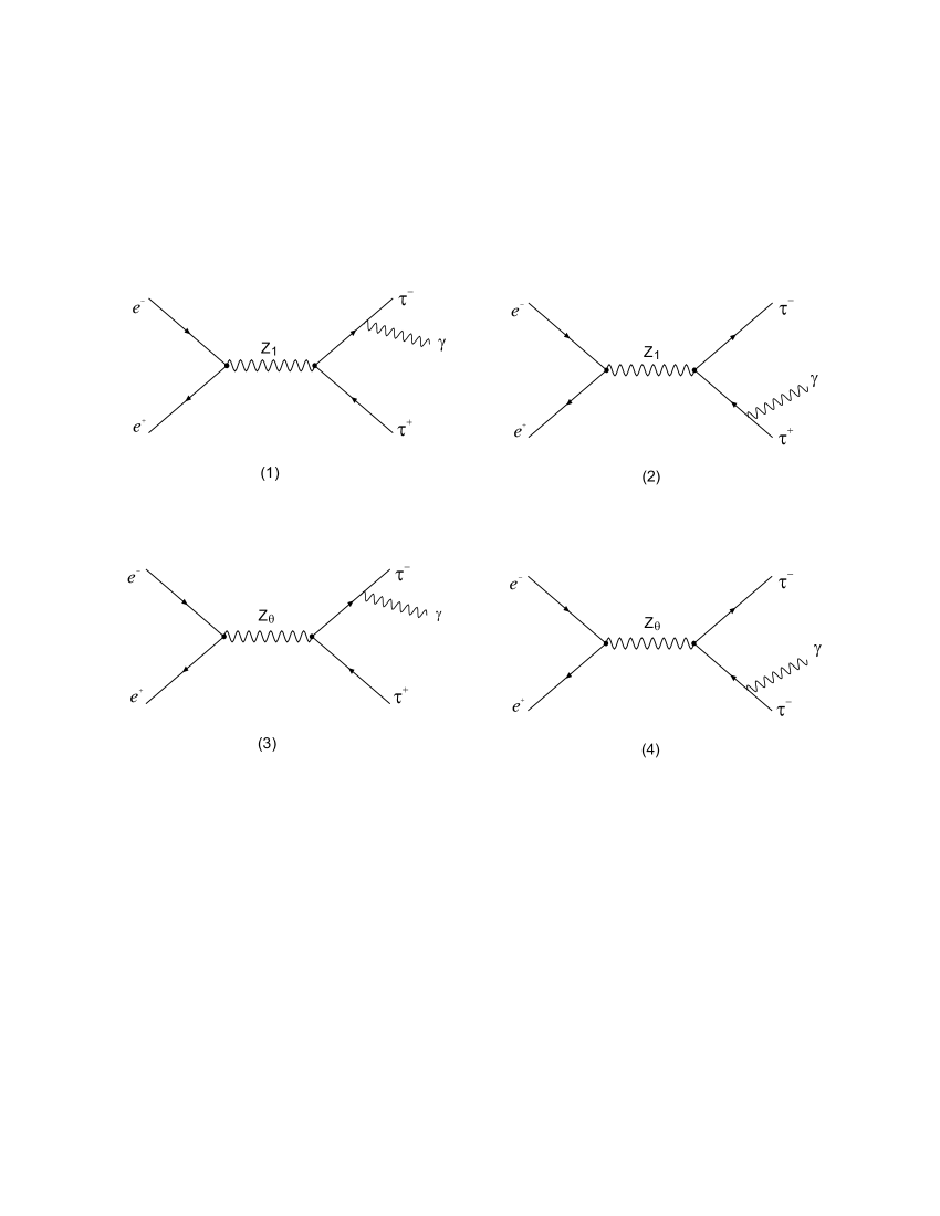
Figure 1: The Feynman diagrams contributing to the process $e^{+}e^{-}\rightarrow\tau^{+}\tau^{-}\gamma$ in a left-right symmetric model, and in the $E_{6}$ model.

On the $Z_{1}$ peak, where a large number of $Z_{1}$ events are collected at $e^{+}e^{-}$ colliders, one may hope to constrain or eventually measure the electromagnetic and weak dipole moments of the $\tau$ by selecting $\tau^{+}\tau^{-}$ events accompanied by a hard photon. The Feynman diagrams which give the most important contribution to the cross section from $e^{+}e^{-}\rightarrow\tau^{+}\tau^{-}\gamma$ are shown in Fig. 1. The total cross section of $e^{+}e^{-}\rightarrow\tau^{+}\tau^{-}\gamma$ will be evaluated at the $Z_{1}$-pole in the framework of a left-right symmetric model and a class of $E_{6}$ inspired models. The numerical computation for the anomalous magnetic and the electric dipole moments of the tau is done using the data collected by the L3 and OPAL Collaborations at LEP L3 ; OPAL . We are interested in studying the effects induced by the effective couplings associated to the weak and electromagnetic moments of the tau lepton given in Eq. (1). For this purpose we will take the respective anomalous vertices $\tau\tau\gamma$ and $\tau\tau Z$, one at the time, in diagrams (1) and (2) of Fig. 1. The numerical computation for the respective transition amplitudes will be done using the data collected by these collaborations.

Our aim in this paper is to analyze the reaction $e^{+}e^{-}\rightarrow\tau^{+}\tau^{-}\gamma$ in the $Z_{1}$ boson resonance. The analysis is carried out in the context of a left-right symmetric model A.Gutierrez ; A.Gutierrez3 and a class of $E_{6}$ inspired models with an additional neutral vector boson $Z_{\theta}$ Aytekin ; Aydin and we attribute a weak and electromagnetic dipole moments to the tau lepton. Processes measured in the resonance serve to set limits on the tau electromagnetic and weak dipole moments. First, using as an input the results obtained by the L3 and OPAL Collaborations L3 ; OPAL for the tau MM and EDP in the process $e^{+}e^{-}\to\tau^{+}\tau^{-}\gamma$, we will set a limit on the LRSM mixing angle $\phi$ which is similar to that obtained recently from the LEP data on the number of light neutrino species A.Gutierrez2 but it is stronger by about one order of magnitude than the previous limit for this angle obtained from old LEP data M.Maya . We then use this limit on $\phi$ to get bounds on the weak dipole moments of the tau from the same L3/OPAL data. We have found that these limits are consistent with the new bounds obtained by the DELPHI and ALEPH Collaborations from the process $e^{+}e^{-}\to\tau^{+}\tau^{-}$ L3E ; DELPHI ; ALEPH . We will get also similar bounds for these dipole moments using the known limits for the $E_{6}$ mixing angle $\phi_{(SM-E_{6})}$ between $Z_{1}$ and $Z_{\theta}$ London ; Capstick .

This paper is organized as follows: In Sect. II we describe the neutral current couplings in $E_{6}$. In Sect. III we present the calculation of the cross section for the process $e^{+}e^{-}\rightarrow\tau^{+}\tau^{-}\gamma$. In Sect. IV we present our results for the numerical computations and, finally, we present our conclusions in Sect. V.

II Neutral Current Couplings in $E_{6}$

In this section we describe the neutral current couplings involved in the class of $E_{6}$ inspired models we are interested in. Let us consider the following breakdown pattern in $E_{6}$:

$$E_{6}\to SO(10)\times U(1)_{\psi}\to SU(5)\times U(1)_{\chi}\times U(1)_{\psi}\to SM\times U(1)_{\theta_{E_{6}}},$$ (2)

where the $SU(3)_{C}\times SU(2)_{L}\times U(1)_{Y_{W}}$ groups of the standard model are embeded in the $SU(5)$ subgroup of $SO(10)$. The couplings of the fermions to the standard model $Z_{1}$ are given, as usual, by

$$Q=I_{3L}-Q_{em}\sin^{2}\theta_{W},$$ (3)

while the couplings to the $Z_{\theta}$ are given by linear combinations of the $U(1)_{\chi}$ and $U(1)_{\psi}$ charges London ; Capstick :

$$Q^{\prime} = Q_{\chi}\cos\theta_{E_{6}}+Q_{\psi}\sin\theta_{E_{6}},$$

$$Q^{\prime\prime} = -Q_{\chi}\sin\theta_{E_{6}}+Q_{\psi}\cos\theta_{E_{6}},$$ (4)

where the operators $Q_{\psi}$ and $Q_{\chi}$ are orthogonal to those of $Q_{em}$ and that of the standard model $Z_{1}$ and $\theta_{E_{6}}$ is the $Q_{\chi}-Q_{\psi}$ mixing angle in $E_{6}$.

With the extra $Z_{\theta}$ neutral vector boson the neutral current Lagrangian is Leike ; Alam

$${-\cal L}_{NC}=eA^{\mu}J_{em\mu}+g_{1}Z^{\mu}_{1}J_{Z_{1}\mu}+g_{2}Z^{\mu}_{\theta}J_{Z_{\theta}\mu},$$ (5)

where $J_{em\mu}$, $J_{Z_{1}\mu}$ and $J_{Z_{\theta}\mu}$ are the electromagnetic current, the $Z_{1}$ current of the standard model and the $J_{Z_{\theta}\mu}$ current of the new boson, respectively and are given by

$$J_{Z_{1}\mu} = \sum_{f}\bar{f}\gamma_{\mu}(C^{1}_{V}+C^{1}_{A}\gamma_{5})f,$$

$$J_{Z_{\theta}\mu} = \sum_{f}\bar{f}\gamma_{\mu}(C^{\prime}_{V}+C^{\prime}_{A}\gamma_{5})f,$$ (6)

where $f$ represents fermions, while

$$g_{1} = (g^{2}+g^{\prime 2})^{1/2}=\frac{e}{2\sin\theta_{W}\cos\theta_{W}},$$

$$g_{2} = g_{\theta},$$ (7)

$$C^{1e}_{V} = -\frac{1}{2}+2\sin^{2}{\theta_{W}},\hskip 28.45274ptC^{1e}_{A}=-\frac{1}{2},$$

$$C^{1\tau}_{V} = -\frac{1}{2}+2\sin^{2}{\theta_{W}},\hskip 28.45274ptC^{1\tau}_{A}=-\frac{1}{2},$$ (8)

$$C^{{}^{\prime}e}_{V} = z^{1/2}(\frac{\cos\theta_{E_{6}}}{\sqrt{6}}+\frac{\sin\theta_{E_{6}}}{\sqrt{10}}),\hskip 25.60747ptC^{{}^{\prime}e}_{A}=2z^{1/2}\frac{\sin\theta_{E_{6}}}{\sqrt{10}},$$

$$C^{{}^{\prime}\tau}_{V} = z^{1/2}(\frac{\cos\theta_{E_{6}}}{\sqrt{6}}+\frac{\sin\theta_{E_{6}}}{\sqrt{10}}),\hskip 25.60747ptC^{{}^{\prime}\tau}_{A}=2z^{1/2}\frac{\sin\theta_{E_{6}}}{\sqrt{10}},$$ (9)

with

$$z=(\frac{g^{2}_{\theta}}{g^{2}+g^{\prime 2}})(\frac{M_{Z_{1}}}{M_{Z_{\theta}}})^{2},$$ (10)

a parameter that depends on the coupling constant $g_{\theta}$ and $M_{Z_{\theta}}$.

The class of $E_{6}$ models we shall be interested in arise with the following specific values for the mixing angle $\theta_{E_{6}}$ London :

$$\theta_{E_{6}} = 0^{o},\hskip 17.07164ptZ_{\theta_{E_{6}}}\to Z_{\psi},$$

$$\theta_{E_{6}} = 37.8^{o},\hskip 17.07164ptZ_{\theta_{E_{6}}}\to Z^{\prime},$$

$$\theta_{E_{6}} = 90^{o},\hskip 17.07164ptZ_{\theta_{E_{6}}}\to Z_{\chi},$$ (11)

$$\theta_{E_{6}} = 127.8^{o},\hskip 17.07164ptZ_{\theta_{E_{6}}}\to Z_{I},$$

where $Z_{\psi}$ is the extra neutral gauge boson arising in $E_{6}\to SO(10)\times U(1)_{\psi}$, $Z^{\prime}$ corresponds to the respective neutral gauge boson obtained if $E_{6}$ is broken down to a rank-5 group, $Z_{\chi}$ is the neutral gauge boson involved in $SO(10)\to SU(5)\times U(1)_{\chi}$, and $Z_{I}$ is the neutral gauge boson associated to the breaking of $E_{6}$ via a non-Abelian discrete symmetry to a rank-5 group London .

The $Z_{\theta}$ can also mix with the standard model $Z_{1}$ so that the physical fields, $Z_{1p}$ and $Z_{\theta p}$ are linear combinations of the gauge fields $Z_{1n}$ and $Z_{\theta n}$ with mixing angle $\phi_{(SM-E_{6})}$. This mixing will alter the fermion couplings to the $Z_{1}$ as is indicated in Eqs. (3a) and (3b) of Ref. Capstick . Since $\phi_{(SM-E_{6})}$ comes from the diagonalization of the $Z_{1}-Z_{\theta}$ mass matrix, it can be expressed in terms of the standard model prediction for the $Z_{1}$ mass, $M_{SM}=M_{W}\cos^{2}\theta_{W}$ and the physical $Z_{1}$ and $Z_{\theta}$ masses Langacker :

$$\tan^{2}\phi_{(SM-{E_{6}})}=\frac{M^{2}_{SM}-M^{2}_{Z_{1}p}}{M^{2}_{Z_{\theta}p}-M^{2}_{Z_{1}p}}.$$ (12)

The bounds of the MM and EDM of the tau lepton, with the modification of the fermion couplings to the $Z_{1}$ to incorporate the mixing of $Z_{1}$ and $Z_{\theta}$ for different values of the mixing angle $\phi_{(SM-E_{6})}$ of the $E_{6}$ model are given in section IV.

III The Total Cross Section

We will take advantage of our previous work on the LRSM and we will calculate the total cross section for the reaction $e^{+}e^{-}\rightarrow\tau^{+}\tau^{-}\gamma$ using the transition amplitudes given in Eqs. (21) and (22) of Ref. A.Gutierrez for the LRSM for diagrams 1 and 2 of Fig. 1. For the contribution coming from diagrams 3 and 4 of Fig. 1, we use Eqs. (6) and (9) given in section II for the $E_{6}$ model. The respective transition amplitudes are thus given by

$${\cal M}_{1} = \frac{-g^{2}}{4\cos^{2}\theta_{W}(l^{2}-m^{2}_{\tau})}[\bar{u}(p_{3})\Gamma^{\alpha}(l\hbox to0.0pt{\hss/}+m_{\tau})\gamma^{\beta}(aC^{1\tau}_{V}-bC^{1\tau}_{A}\gamma_{5})v(p_{4})]$$ (13)

$$\frac{(g_{\alpha\beta}-p_{\alpha}p_{\beta}/M^{2}_{Z_{1}})}{[(p_{1}+p_{2})^{2}-M^{2}_{Z_{1}}-i\Gamma^{2}_{Z_{1}}]}[\bar{u}(p_{2})\gamma^{\alpha}(aC_{V}^{1e}-bC_{A}^{1e}\gamma_{5})v(p_{1})]\epsilon^{\lambda}_{\alpha},$$

$${\cal M}_{2} = \frac{-g^{2}}{4\cos^{2}\theta_{W}(k^{2}-m^{2}_{\tau})}[\bar{u}(p_{3})\gamma^{\beta}(aC^{1\tau}_{V}-bC^{1\tau}_{A}\gamma_{5})(k\hbox to0.0pt{\hss/}+m_{\tau})\Gamma^{\alpha}v(p_{4})]$$ (14)

$$\frac{(g_{\alpha\beta}-p_{\alpha}p_{\beta}/M^{2}_{Z_{1}})}{[(p_{1}+p_{2})^{2}-M^{2}_{Z_{1}}-i\Gamma^{2}_{Z_{1}}]}[\bar{u}(p_{2})\gamma^{\alpha}(aC_{V}^{1e}-bC_{A}^{1e}\gamma_{5})v(p_{1})]\epsilon^{\lambda}_{\alpha},$$

and for $M^{\prime}_{1}$ and $M^{\prime}_{2}$

$$M^{\prime}_{1} = M_{1}(aC^{1}_{V}\to C_{V}^{\prime},bC^{1}_{A}\to C_{A}^{\prime},M_{Z_{1}}\to M_{Z_{\theta}}),$$ (15)

$$M^{\prime}_{2} = M_{2}(aC^{1}_{V}\to C_{V}^{\prime},bC^{1}_{A}\to C_{A}^{\prime},M_{Z_{1}}\to M_{Z_{\theta}}),$$ (16)

where $\Gamma^{\alpha}$ is the tau-lepton electromagnetic vertex which is defined in the Eq. (1), while $\epsilon^{\lambda}_{\alpha}$ is the polarization vector of the photon. $l$ ($k$) stands for the momentum of the virtual tau (antitau), and the coupling constants $a$ and $b$ are given in the Eq. (16) of the Ref. A.Gutierrez , while $C^{\prime}_{V}$ and $C^{\prime}_{A}$ are given above in the Eq. (9).

The MM, EDM, the mixing angle $\phi$ of the LRSM as well as the mixing angle $\theta_{E_{6}}$ and the mass of the additional neutral vector boson $M_{Z_{\theta}}$ of the $E_{6}$ model give a contribution to the differential cross section for the process $e^{+}e^{-}\rightarrow\tau^{+}\tau^{-}\gamma$ of the form:

$$\frac{d\sigma}{E_{\gamma}dE_{\gamma}d\cos\theta_{\gamma}} = \frac{\alpha^{2}}{48\pi}\;\{[\frac{e^{2}a^{2}_{\tau}}{4m^{2}_{\tau}}+d^{2}_{\tau}]\;[{\cal C}[\phi,x_{W}]\;{\cal F}[\phi,s,E_{\gamma},\cos\theta_{\gamma}]$$ (17)

$$+ {\cal C}_{1}[\theta_{E_{6}},M_{Z_{\theta}},x_{W}]\;{\cal F}_{1}[M_{Z_{\theta}},s,E_{\gamma},\cos\theta_{\gamma}]+8f[M_{Z_{1}},\Gamma_{Z_{1}},M_{Z_{\theta}},\Gamma_{Z_{\theta}}]$$

$$\cdot \{{\cal C}_{2}[\phi,\theta_{E_{6}},M_{Z_{\theta}},x_{W}]\;{\cal F}_{2}[s]+{\cal C}_{3}[\phi,\theta_{E_{6}},M_{Z_{\theta}},x_{W}]\;{\cal F}_{3}[s,E_{\gamma}]+{\cal C}_{4}[\theta_{E_{6}},M_{Z_{\theta}}]\;{\cal F}_{4}[E_{\gamma}]$$

$$+ {\cal C}_{5}[\phi,\theta_{E_{6}},M_{Z_{\theta}},x_{W}]\;{\cal F}_{5}[s,E_{\gamma},\cos\theta_{\gamma}]+{\cal C}_{6}[\phi,\theta_{E_{6}},M_{Z_{\theta}},x_{W}]\;{\cal F}_{6}[s,E_{\gamma},\cos\theta_{\gamma}]\}]$$

$$+ \frac{3}{32}[\frac{ea_{\tau}}{2m_{\tau}}+d_{\tau}]\;f[M_{Z_{1}},\Gamma_{Z_{1}},M_{Z_{\theta}},\Gamma_{Z_{\theta}}]\cdot\{{\cal C}_{7}[\phi,M_{Z_{\theta}},x_{W}]\;{\cal F}_{7}[s,E_{\gamma},\cos\theta_{\gamma}]$$

$$- {\cal C}_{7}[\phi,M_{Z_{\theta}},x_{W}]\;{\cal F}_{8}[s,E_{\gamma},\cos\theta_{\gamma}]-{\cal C}_{8}[\phi,M_{Z_{\theta}},x_{W}]\;{\cal F}_{7}[s,E_{\gamma},\cos\theta_{\gamma}]$$

$$+ {\cal C}_{8}[\phi,M_{Z_{\theta}},x_{W}]\;{\cal F}_{8}[s,E_{\gamma},\cos\theta_{\gamma}]\}+\frac{1}{36}{\cal C}_{9}[x_{W}]\;{\cal F}_{9}[s,E_{\gamma},\cos\theta_{\gamma}]\},$$

where $E_{\gamma}$, $\cos\theta_{\gamma}$ are the energy and the opening angle of the emmited photon.

The kinematics is contained in the functions

$${\cal F}[\phi,s,E_{\gamma},\cos\theta_{\gamma}] \equiv \frac{[[\frac{1}{2}(a^{2}+b^{2})-4a^{2}x_{W}+8a^{2}x^{2}_{W}](s-2\sqrt{s}E_{\gamma})+\frac{1}{2}b^{2}E^{2}_{\gamma}\sin^{2}\theta_{\gamma}]}{[(s-M_{Z_{1}}^{2})^{2}+M^{2}_{Z_{1}}\Gamma^{2}_{Z_{1}}]},$$

$${\cal F}_{1}[M_{Z_{\theta}},s,E_{\gamma},\cos\theta_{\gamma}] \equiv \frac{[[(C^{{}^{\prime}\tau}_{V})^{2}+(C^{{}^{\prime}\tau}_{A})^{2}](s-2\sqrt{s}E_{\gamma})+(C^{{}^{\prime}\tau}_{A})^{2}E^{2}_{\gamma}\sin^{2}\theta_{\gamma}]}{[(s-M_{Z_{\theta}}^{2})^{2}+M^{2}_{Z_{\theta}}\Gamma^{2}_{Z_{\theta}}]},$$

$${\cal F}_{2}[s] \equiv 4\sqrt{s},$$

$${\cal F}_{3}[s,E_{\gamma}] \equiv 2\sqrt{s}E_{\gamma},$$

$${\cal F}_{4}[E_{\gamma}] \equiv \sqrt{15}E_{\gamma},$$

$${\cal F}_{5}[s,E_{\gamma},\cos\theta_{\gamma}] \equiv -(s+\frac{1}{2}E^{2}_{\gamma}\sin^{2}\theta_{\gamma}),$$

$${\cal F}_{6}[s,E_{\gamma},\cos\theta_{\gamma}] \equiv (s-E_{\gamma}^{2}+\frac{1}{2}E^{2}_{\gamma}\sin^{2}\theta_{\gamma}),$$ (18)

$${\cal F}_{7}[s,E_{\gamma},\cos\theta_{\gamma}] \equiv (12\sqrt{s}E_{\gamma}+9E^{2}_{\gamma}\sin^{2}\theta_{\gamma}),$$

$${\cal F}_{8}[s,E_{\gamma},\cos\theta_{\gamma}] \equiv (9s+4\sqrt{s}E_{\gamma}\sin^{2}\theta_{\gamma}),$$

$${\cal F}_{9}[s,E_{\gamma},\cos\theta_{\gamma}] \equiv \frac{[4\sqrt{s}-2E_{\gamma}\sin^{2}\theta_{\gamma}-\sqrt{s}\sin^{2}\theta_{\gamma}]}{[(s-M_{Z_{1}}^{2})^{2}+M^{2}_{Z_{1}}\Gamma^{2}_{Z_{1}}]},$$

$$f(s,M_{Z_{1}},\Gamma_{Z_{1}},M_{Z_{\theta}},\Gamma_{Z_{\theta}})$$

$$\equiv \frac{-2[(s-M^{2}_{Z_{1}})(s-M^{2}_{Z_{\theta}})+M_{Z_{1}}\Gamma_{Z_{1}}M_{Z_{\theta}}\Gamma_{Z_{\theta}}]}{[(s-M^{2}_{Z_{1}})(s-M^{2}_{Z_{\theta}})+M_{Z_{1}}\Gamma_{Z_{1}}M_{Z_{\theta}}\Gamma_{Z_{\theta}}]^{2}+[(s-M^{2}_{Z_{\theta}})M_{Z_{1}}\Gamma_{Z_{1}}-(s-M^{2}_{Z_{1}})M_{Z_{\theta}}\Gamma_{Z_{\theta}}]^{2}}.$$

The coefficients ${\cal C}$, ${\cal C}_{1}$,…, ${\cal C}_{9}$ are given by

$${\cal C}[\phi,x_{W}] \equiv \frac{[\frac{1}{2}(a^{2}+b^{2})-4a^{2}x_{W}+8a^{2}x^{2}_{W}]}{x^{2}_{W}(1-x_{W})^{2}},$$

$${\cal C}_{1}[\theta_{E_{6}},M_{Z_{\theta}},x_{W}] \equiv \frac{3[(C^{{}^{\prime}e}_{V})^{2}+(C^{{}^{\prime}e}_{A})^{2}]}{x^{2}_{W}(1-x_{W})^{2}},$$

$${\cal C}_{2}[\phi,\theta_{E_{6}},M_{Z_{\theta}},x_{W}] \equiv \frac{[2ax_{W}-\frac{1}{2}(a-b)][C_{V}^{{}^{\prime}e}C_{A}^{{}^{\prime}e}-(C_{A}^{{}^{\prime}e})^{2}]}{x^{2}_{W}(1-x_{W})^{2}},$$

$${\cal C}_{3}[\phi,\theta_{E_{6}},M_{Z_{\theta}},x_{W}] \equiv \frac{[4ax_{W}-a][3(C_{A}^{{}^{\prime}e})^{2}-(C_{V}^{{}^{\prime}e}-C_{A}^{{}^{\prime}e})^{2}]}{x^{2}_{W}(1-x_{W})^{2}}$$

$${\cal C}_{4}[\theta_{E_{6}},M_{Z_{\theta}},x_{W}] \equiv \frac{[3(C_{A}^{{}^{\prime}e})^{2}+(C_{V}^{{}^{\prime}e}-C_{A}^{{}^{\prime}e})^{2}]}{x^{2}_{W}(1-x_{W})^{2}},$$ (19)

$${\cal C}_{5}[\phi,\theta_{E_{6}},M_{Z_{\theta}},x_{W}] \equiv \frac{[3(C_{A}^{{}^{\prime}e})^{2}(4ax_{W}-a+\frac{1}{2})+[4ax_{W}-(a-b)][C_{V}^{{}^{\prime}e}C_{A}^{{}^{\prime}e}-(C_{A}^{{}^{\prime}e})^{2}]]}{x^{2}_{W}(1-x_{W})^{2}},$$

$${\cal C}_{6}[\phi,\theta_{E_{6}},M_{Z_{\theta}},x_{W}] \equiv \frac{[2ax_{W}-\frac{1}{2}a](C_{V}^{{}^{\prime}e}-C_{A}^{{}^{\prime}e})^{2}}{x^{2}_{W}(1-x_{W})^{2}},$$

$${\cal C}_{7}[\phi,M_{Z_{\theta}},x_{W}] \equiv \frac{[\frac{1}{2}(a^{2}+b^{2})-4a^{2}x_{W}+8a^{2}x^{2}_{W}][\frac{1}{2}(a+b)-4ax_{W}+8ax^{2}_{W}]}{x^{2}_{W}(1-x_{W})^{2}},$$

$${\cal C}_{8}[\phi,\theta_{E_{6}},M_{Z_{\theta}},x_{W}] \equiv \frac{[\frac{1}{2}(a^{2}+b^{2})-4a^{2}x_{W}+8a^{2}x^{2}_{W}][(1-4x_{W})C_{V}^{{}^{\prime}\tau}-C_{A}^{{}^{\prime}\tau}]}{x^{2}_{W}(1-x_{W})^{2}},$$

$${\cal C}_{9}[x_{W}] \equiv \frac{[1-4x_{W}+8x^{2}_{W}]^{2}}{x^{2}_{W}(1-x_{W})^{2}},$$

with $x_{W}\equiv\sin^{2}\theta_{W}$.

In the above expressions, the function ${\cal F}$ includes the contribution coming from the exchange of the SM/LRSM $Z_{1}$ gauge boson, ${\cal F}_{1}$ includes the contribution arising from the exchange of the heavy gauge boson $Z_{\theta}$, while the function $f$ contains the interference coming from both exchanges. Taking the limit when $M_{Z_{\theta}}\to\infty$ and the mixing angle $\phi=0$, the expressions for $C_{V}^{{}^{\prime}e,\tau}$ and $C_{A}^{{}^{\prime}e,\tau}$ reduce to $C_{V}^{{}^{\prime}e,\tau}=C_{A}^{{}^{\prime}e,\tau}=0$ and, Eq. (17) reduces to the expression (4) given in Ref. Grifols for the SM. On the other hand, taking the limit when $M_{Z_{\theta}}\to\infty$ the Eq. (17) reduces to the expressions (25) given in Ref. A.Gutierrez for the LRSM. Finally, if the mixing angle is taken as $\phi=0$, Eq. (17) reduces to the expression for the SM-$E_{6}$ models.

In the case of the weak dipole moments, to get the expression for the differential cross section, we have to substitute the $Z$ SM couplings given in Eq. (8) by the respective weak dipole moments included in Eq. (1), that is to say $a^{W}_{\tau}=F^{Z}_{2}(q^{2}=m^{2}_{Z})$ and $d^{W}_{\tau}=eF^{Z}_{3}(q^{2}=m^{2}_{Z})$. We do not reproduce the analytical expressions here because they are rather similar to the terms given in Eqs. (17-19). We applied a similar analysis recently A.Gutierrez1 in order to get bounds on the MM and EDM associated to the tau-neutrino using the L3 data obtained for the reaction $e^{+}e^{-}\rightarrow\nu\bar{\nu}\gamma$ L3E . In the following section we will present the bounds obtained for the tau dipole moments using the data published by the L3 and OPAL Collaborations for the reaction $e^{+}e^{-}\rightarrow\tau^{+}\tau^{-}\gamma$ L3 ; OPAL .

IV Results

In practice, detector geometry imposes a cut on the photon polar angle with respect to the electron direction, and further cuts must be applied on the photon energy and minimum opening angle between the photon and tau in order to suppress background from tau decay products. In order to evaluate the integral of the total cross section as a function of the parameters of the LRSM-$E_{6}$ models, that is to say, $\phi$, $M_{Z_{\theta}}$ and the mixing angle $\theta_{E_{6}}$, we require cuts on the photon angle and energy to avoid divergences when the integral is evaluated at the important intervals of each experiment. We integrate over $\cos\theta_{\gamma}$ from $-0.74$ to $0.74$ and $E_{\gamma}$ from 5 $GeV$ to 45.5 $GeV$ for various fixed values of the mixing angle $\phi=-0.00166,0,0.00122$ (as is illustrate in Fig. 2) and for $\theta_{E_{6}}=37.8^{o}$ (which corresponds to $Z_{\theta}\to Z^{\prime}$) and $M_{Z_{\theta}}=7M_{Z_{1}}$ according to Ref. Aytekin . Using the following numerical values: $\sin^{2}\theta_{W}=0.2314$, $M_{Z_{1}}=91.18$ $GeV$, $\Gamma_{Z_{\theta}}=\Gamma_{Z_{1}}=2.49$ $GeV$ and $z=(\frac{3}{5}\sin^{2}\theta_{W})(\frac{M_{Z_{1}}}{M_{Z_{\theta}}})^{2}$ we obtain the cross section $\sigma=\sigma(\phi,\theta_{E_{6}},M_{Z_{\theta}},a_{\tau},d_{\tau})$.

In Fig. 2, we show the dependence of the total cross section for the process $e^{+}e^{-}\to\tau^{+}\tau^{-}\gamma$ with respect to the LRSM mixing angle $\phi$. Using the limits obtained by the L3/OPAL Collaborations L3 ; OPAL for this process, we get the following limits for $\phi$

$$-1.66\times 10^{-3}\leq\phi\leq 1.22\times 10^{-3},$$ (20)

which are consistent with those obtained recently from the LEP data on the number of light neutrino species in the LRSM A.Gutierrez2 , and they are about one order of magnitude stronger than the previous limit obtained from old LEP data M.Maya . Since we have calculated the cross section at the $Z_{1}$ pole, i.e. at $s=M^{2}_{Z_{1}}$, the value of $\sin^{2}\theta_{W}$ is not affected by the $Z_{\theta}$ physics Langacker1 ; Demir . Variation of the $\Gamma_{Z_{\theta}}$ is taken in the range from 0.15 to 2.0 times $\Gamma_{Z_{1}}$ in the results of the CDF Collaboration CDF . So we take $\Gamma_{Z_{\theta}}=\Gamma_{Z_{1}}$ as a special case of this variation.

As was discussed in Ref. L3 , $N\approx\sigma(\phi,\theta_{E_{6}},M_{Z_{\theta}},a_{\tau},d_{\tau}){\cal L}$, using Poisson statistic L3 ; Barnett , we require that $N\approx\sigma(\phi,\theta_{E_{6}},M_{Z_{\theta}},\mu_{\nu_{\tau}},d_{\nu_{\tau}}){\cal L}$ be less than 1559, with ${\cal L}=100$ $pb^{-1}$, according to the data reported by the L3 Collaboration Ref. L3 and references therein. Taking this into consideration, we can get a bound for the tau magnetic moment as a function of $\phi$, $\theta_{E_{6}}$ and $M_{Z_{\theta}}$ with $d_{\tau}=0$. The values obtained for this bound for several values of $\phi$ with $\theta_{E_{6}}=37.8^{o}$ and $M_{Z_{\theta}}=7M_{Z_{1}}$ are included in Table 1. The previous analysis and comments can readily be translated to the EDM of the tau with $a_{\tau}=0$. The resulting bounds for the EDM as a function of $\phi$, $\theta_{E_{6}}$ and $M_{Z_{\theta}}$ are shown in Table 1. As expected, the limits obtained for the electromagnetic dipole moments of the tau lepton are consistent with those obtained by the these collaborations from the data obtained for the process $e^{+}e^{-}\to\tau^{+}\tau^{-}\gamma$ L3 ; OPAL .

$\phi$	${a_{\tau}}$	$d_{\tau}(10^{-16}e\mbox{cm})$
$-1.66\times 10^{-3}$	0.0521	2.891
0	0.052	2.885
$1.22\times 10^{-3}$	0.0519	2.881

Table 1. Limits on the $a_{\tau}$ MM and $d_{\tau}$ EDM of the $\tau$-lepton for different values of the mixing angle $\phi$ with $\theta_{E_{6}}=37.8^{o}$ and $M_{Z_{\theta}}=7M_{Z_{1}}$. We have applied the cuts used by L3 for the photon angle and energy.

The bounds for the weak dipole moments of the tau-lepton according to the data from the L3 and OPAL Collaboration L3 ; OPAL for the energy and the opening angle of the photon, as well as the luminosity and the events numbers are given in the Table 2. As we can appreciate, the use of the strong limit obtained for the $\phi$ mixing angle induces also stringet bounds for the tau weak dipole moments, which are already consistent with those bound recently by the DELPHI and ALEPH Collaborations in the process $e^{+}e^{-}\to\tau^{+}\tau^{-}$ DELPHI ; ALEPH .

$\phi$	${a^{W}_{\tau}(10^{-3})}$	$d^{W}_{\tau}(10^{-17}e\mbox{cm})$
$-1.66\times 10^{-3}$	2.143	1.19
0	2.138	1.187
$1.22\times 10^{-3}$	2.135	1.185

Table 2. Limits on the $a^{W}_{\tau}$ anomalous weak MM and $d^{W}_{\tau}$ weak EDM of the $\tau$-lepton for different values of the mixing angle $\phi$. We have applied the cuts used by L3 for the photon angle and energy.

As far as the respective analysis for the $E_{6}$ model is concerned, we will use the known limits for the mixing angle $\phi_{(SM-E_{6})}$ London ; Capstick ,

$$-0.054\leq\phi_{(SM-E_{6})}\leq 0.054,$$ (21)

in order to get the respective limits of the tau dipole moments. In Tables 3 and 4 we show these limits. Here we obtain also limits for the electromagnetic moments that are consistent with the old results published by the L3/OPAL Collaborations L3 ; OPAL , but our limits for the weal dipole moments are consistent with the data published recently by the DELPHI/ALEPH Collaborations.

$\phi_{(SM-E_{6})}$	${a_{\tau}}$	$d_{\tau}(10^{-16}e\mbox{cm})$
-0.054	0.047	2.64
0	0.052	2.88
0.054	0.054	2.92

Table 3. Limits on the $a_{\tau}$ MM and $d_{\tau}$ EDM of the $\tau$-lepton for different values of the mixing angle $\phi_{(SM-E_{6})}$ with $\theta_{E_{6}}=37.8^{o}$ and $M_{Z_{\theta}}=7M_{Z_{1}}$. We have applied the cuts used by L3 for the photon angle and energy.

$\phi_{(SM-E_{6})}$	${a^{W}_{\tau}(10^{-3})}$	$d^{W}_{\tau}(10^{-17}e\mbox{cm})$
-0.054	1.91	1.08
0	2.13	1.18
0.054	2.20	1.22

Table 4. Limits on the $a^{W}_{\tau}$ anomalous weak MM and $d^{W}_{\tau}$ weak EDM of the $\tau$-lepton for different values of the mixing angle $\phi_{(SM-E_{6})}$. We have applied the cuts used by L3 for the photon angle and energy.

We plot the total cross section in Fig. 3 as a function of the mixing angle $\phi$ for the bounds of the magnetic moment given in Table 1 with $\theta_{E_{6}}=37.8^{0}$ and $M_{Z_{\theta}}=7M_{Z_{1}}$. We reproduce the Fig. 2 of the Ref. A.Gutierrez . Our results for the dependence of the differential cross section on the photon energy versus the cosine of the opening angle between the photon and the beam direction ($\theta_{\gamma}$) are presented in Fig. 4, for $\phi=0.00122$ and $a_{\tau}=0.0519$. In this case also we reproduce the Fig. 3 of the Ref. A.Gutierrez . Finally we plot the differential cross section in Fig. 5 as a function of the photon energy for the bounds of the magnetic moments given in Table 1. We observed in this figure that the energy distributions are consistent with those reported in the literature.

In a previous paper A.Gutierrez we estimated bounds on the anomalous magnetic moment and the electric dipole moment of the tau through the process $e^{+}e^{-}\rightarrow\tau^{+}\tau^{-}\gamma$ in the context of a LRSM at the $Z_{1}$ pole. We found that these bound were almost independent of the mixing angle $\phi$ of the model. In the present paper we reproduce these bounds for $\theta_{E_{6}}=37.8^{o}$ and $M_{Z_{\theta}}=7M_{Z_{1}}$ Aytekin , corresponding to the $E_{6}$ superstring models. Our results in Table 2 for $\phi=-0.00166,0,0.00122$ and Table 4 for $\phi_{(SM-E_{6})}=-0.054,0,0.054$ with $\theta_{E_{6}}=37.8^{o}$ and $M_{Z_{\theta}}=7M_{Z_{1}}$ confirm the bounds obtained by the DELPHI and ALEPH collaborations for the weak tau dipole moments Lohmann ; DELPHI ; ALEPH ; however, our analysis is not sensitive to the real and imaginary parts of these parameters separately. On the other hand, it seems that in order to improve these limits it might be necessary to study direct CP-violating effects M.A.Perez ; Larios .

V Conclusions

We have determined limits on the electromagnetic and weak dipole moments of the tau lepton using the data published by the L3 and OPAL Collaborations for the process $e^{+}e^{-}\to\tau^{+}\tau^{-}\gamma$. We were able to get strong limits on the weak dipole moments by constraining the LRSM mixing angle $\phi$ from the electromagnetic dipole moments obtained by these collaborations. We then used this limit to constrain the weak dipole moments of the tau lepton from the same L3/OPAL data and we have obtained similar bounds for these dipole moments as those obtained recently by the DELPHI/ALEPH Collaborations from the process $e^{+}e^{-}\to\tau^{+}\tau^{-}$ DELPHI ; ALEPH . We have obtained similar bounds in the case of the $E_{6}$ string models for appropriated values of its parameters. In particular, in the limit $\phi=0$, $\phi_{(SM-E_{6})}=0$ and $M_{Z_{\theta}}\to\infty$, our bound takes the value previously reported in Ref. Grifols for the SM. The bounds in the MM and the EDM are not affected for the additional neutral vector boson $Z_{\theta}$ since its mass is higher than $Z_{1}$ at $\sqrt{s}=M_{Z_{1}}$. But at higher center-of-mass energies $\sqrt{s}\sim M_{Z_{\theta}}$, the $Z_{\theta}$ contribution to the cross section becomes comparable with $Z_{1}$. As far as the weak dipole moments are concerned, our limits given in Tables 1-4 are consistent with the experimental bounds obtained at LEP with the two-body decay mode $Z_{1}\to\tau^{+}\tau^{-}$ Lohmann . In addition, the analytical and numerical results for the total cross section have never been reported in the literature before and could be of relevance for the scientific community.

Acknowledgments

We acknowledge support from CONACyT and SNI (México).

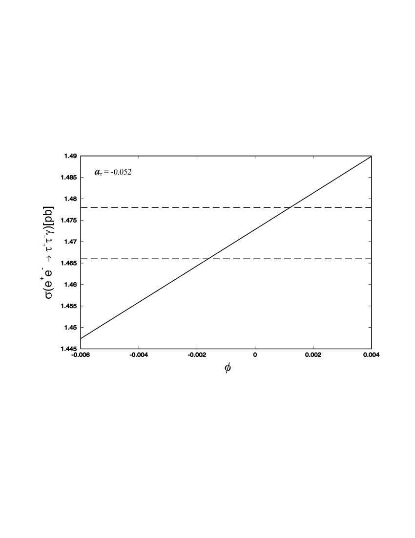
Figure 2: The curves show the shape for $\sigma(e^{+}e^{-}\rightarrow\tau^{+}\tau^{-}\gamma)$ as a function of the mixing angle $\phi$, with $a_{\tau}=-0.052$.

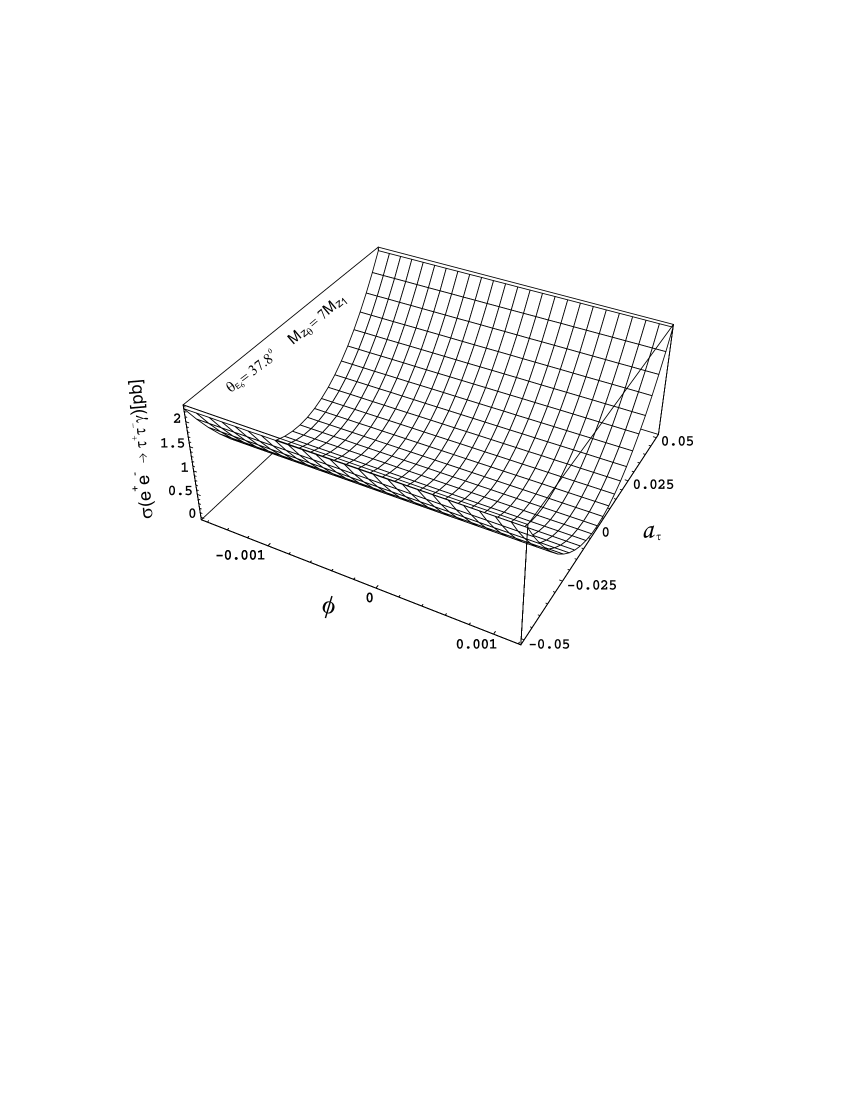
Figure 3: The total cross section for $e^{+}e^{-}\rightarrow\tau^{+}\tau^{-}\gamma$ as a function of $\phi$ and $a_{\tau}$ (Table 1) with $\theta_{E_{6}}=37.8^{o}$ and $M_{Z_{\theta}}=7M_{Z_{1}}$.

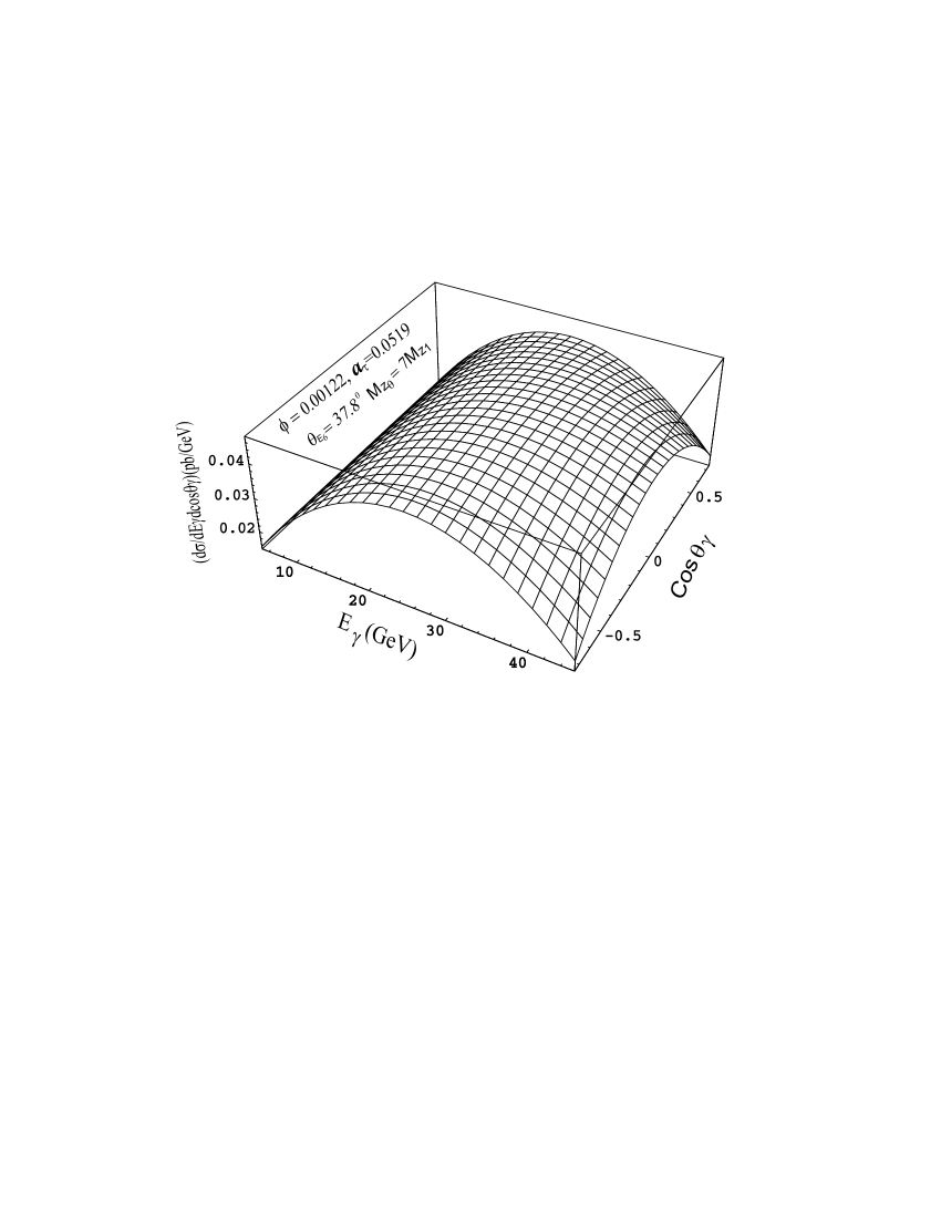
Figure 4: The differential cross section for $e^{+}e^{-}\rightarrow\tau^{+}\tau^{-}\gamma$ as a function of $E_{\gamma}$ and $\cos\theta_{\gamma}$ for $\phi=1.22\times 10^{-3}$, $a_{\tau}=0.0519$, $\theta_{E_{6}}=37.8^{o}$ and $M_{Z_{\theta}}=7M_{Z_{1}}$ .

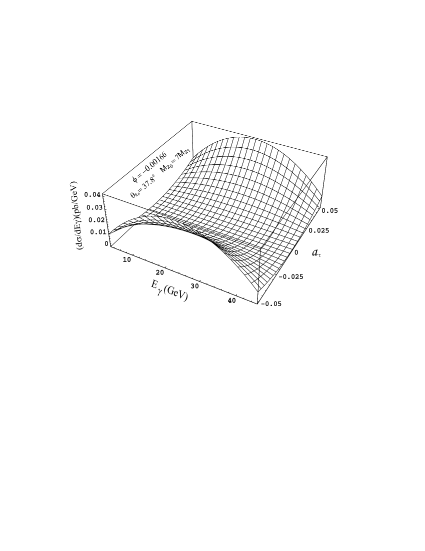
Figure 5: The differential cross section for $e^{+}e^{-}\rightarrow\tau^{+}\tau^{-}\gamma$ as a function of $E_{\gamma}$ and $a_{\tau}$ with $\phi=-1.66\times 10^{-3}$, $\theta_{E_{6}}=37.8^{o}$ and $M_{Z_{\theta}}=7M_{Z_{1}}$.

References

• (1) W. Lohmann, Nucl. Phys. Proc. Suppl. 144, 122 (2005).
• (2) L3 Collab., P. Achard et al., Phys. Lett. B585, 53 (2004).
• (3) DELPHI Collab., J. Abdallah et al., Eur. Phys. J. C35, 159 (2004), and references therein.
• (4) ALEPH Collab., A. Heister et al., Eur. Phys. J. C30, 291 (2003), and references therein.
• (5) S. L. Glashow, Nucl. Phys. 22, 579 (1961).
• (6) S. Weinberg, Phys. Rev. Lett. 19, 1264 (1967).
• (7) A. Salam, in Elementary Particle Theory, Ed. N. Svartholm (Almquist and Wiskell, Stockholm, 1968) 367.
• (8) M. A. Samuel, G. Li and R. Mendel, Phys. Rev. Lett. 67, 668 (1991); Erratum ibid. 69, 995 (1992).
• (9) F. Hamzeh and N. F. Nasrallah, Phys. Lett. B373, 211 (1996).
• (10) S. M. Barr and W. Marciano in CP Violation, ed. C. Jarlskog (World Scientific, Singapore, 1990).
• (11) J. Bernabeu et al., Nucl. Phys. B436, 474 (1995).
• (12) J. Bernabeu et al., Phys. Lett. B326, 168 (1994).
• (13) W. Bernreuther et al. Z. Phys. C43, 117 (1989).
• (14) M. J. Booth, hep-ph/9301293.
• (15) M. C. GonzΓ‘lez-GarcΓ­a and S. F. Novaes, Phys. Lett. B389, 707 (1996).
• (16) P. Poulose and S. D. Rindani, hep-ph/9708332.
• (17) T. Huang, W. Lu and Z. Tao, Phys. Rev. D55, 1643 (1997).
• (18) R. Escribano and E. MassΓ³, Phys. Lett. B395, 369 (1997).
• (19) J.A. Grifols and A. MΓ©ndez, Phys. Lett. B255, 611 (1991); Erratum ibid. B259, 512 (1991).
• (20) L. Taylor, Nucl. Phys. Proc. Suppl. B76, 237 (1999).
• (21) G.A. GonzΓ‘lez-Sprinberg, A. Santamaria, J. Vidal, Int. J. Mod. Phys. A16S1B, 545 (2001).
• (22) Gabriel A. GonzΓ‘lez-Sprinberg, Arcadi Santamaria, Jorge Vidal, Nucl. Phys. Proc. Suppl. 98, 133 (2001).
• (23) Gabriel A. GonzΓ‘lez-Sprinberg, A. Santamaria, J. Vidal, Nucl. Phys. B582, 3 (2000).
• (24) E. O. Iltan, Eur. Phys. J. C44, 411 (2005).
• (25) B. Dutta, R. N. Mohapatra, Phys. Rev. D68, 113008 (2003).
• (26) E. Iltan, Phys. Rev. D64, 013013 (2001).
• (27) E. Iltan, JHEP 065, 0305 (2003).
• (28) E. Iltan, JHEP 0404, 018 (2004).
• (29) R.W. Robinett, Phys. Rev. D26, 2388 (1982).
• (30) R.W. Robinett and J.L. Rosner, Phys. Rev. D25, 3036 (1982); Erratum ibid. D27, 679 (1983).
• (31) R.W. Robinett and J.L. Rosner, Phys. Rev. D26, 2396 (1982).
• (32) P. Langacker, R.W. Robinett and J.L. Rosner, Phys. Rev. D30, 1470 (1984).
• (33) M. Green and J. Schwarz, Phys. Lett. B149, 117 (1984).
• (34) M. Green and J. Schwarz, Phys. Lett. B151, 21 (1985).
• (35) D. Gross et al., Phys. Rev. Lett. 54, 502 (1985).
• (36) E. Witten, Phys. Lett. B155, 1551 (1985).
• (37) E. Witten, Nucl. Phys. B258, 75 (1985).
• (38) P. Candelas et al., ibid B258, 46 (1985).
• (39) M. Dine et al., Nucl. Phys. B259, 549 (1985).
• (40) J. Ellis et al., CERN Report CERN-TH-4350/86 (1986, unpublished).
• (41) J.D. Breit, B. A. Ovrut and G.C. Segre, Phys. Lett. B158, 33 (1985).
• (42) P. Candelas et al., Nucl. Phys. B258, 46 (1985).
• (43) S. Cecotti et al., ibid B156, 318 (1985).
• (44) R. N. Mohapatra and P. B. Pal, in Massive Neutrinos in Physics and Astrophysics, (World Scientific, Singapore, 1991).
• (45) G. Senjanovic, Nucl. Phys. B153, 334 (1979).
• (46) R. Shrock, Nucl. Phys. B206, 359 (1982).
• (47) G. Senjanovic and R. N. Mohapatra, Phys. Rev. D12, 1502 (1975).
• (48) For a review of composite vector bosons see B. Schrempp, Proceedings of the 23rd International Conference on High Energy Physics, Berkeley (World Scientific, Singapore 1987).
• (49) U. Baur et al., Phys. Rev. D35, 297 (1987).
• (50) M. Kuroda et al., Nucl. Phys. B261, 432 (1985).
• (51) L3 Collab., M. Acciarri et al., Phys. Lett. B434, 169 (1998), and references therein.
• (52) OPAL Collab., K. Ackerstaff et al., Phys. Lett. B431, 188 (1998), and references therein.
• (53) A. GutiΓ©rrez-RodrΓ­guez, M. A. HernΓ‘ndez-RuΓ­z and L. N. Luis-Noriega, Mod. Phys. Lett. A19, 2227 (2004).
• (54) A. GutiΓ©rrez-RodrΓ­guez, M. A. HernΓ‘ndez-RuΓ­z and L. N. Luis-Noriega, J. Phys. Conf. Ser. 37, 25 (2006).
• (55) Aytekin Aydemir and Ramazan Sever, Mod. Phys. Lett. A16, 457 (2001).
• (56) C. Aydin, M. Bayar, C. Kilic, hep-ph/0603080.
• (57) A. GutiΓ©rrez-RodrΓ­guez, M. HernΓ‘ndez-RuΓ­z, and M. A. PΓ©rez, hep-ph/0702076.
• (58) M. Maya and O. G. Miranda, Z. Phys. C68, 481 (1995).
• (59) L3 Collab., M. Acciarri et al., Phys. Lett. B412, 201 (1997).
• (60) David London and Jonathan L. Rosner, Phys. Rev. D34, 1530 (1986), and references therein.
• (61) Simon Capstick and Stephen Godfrey, Phys. Rev. D35, 3351 (1987), and references therein.
• (62) A. Leike, Phys. Rep. 317, 143 (1999).
• (63) S. Alam, J. D. Anand, S.N. Biswas and A. Goyal, Phys. Rev. D40, 2712 (1989).
• (64) P. Langacker, Phys. Rev. D30, 2008 (1984)
• (65) A. GutiΓ©rrez-RodrΓ­guez, M. HernΓ‘ndez-RuΓ­z, B. Jayme-ValdΓ©s and M. A. PΓ©rez, Phys. Rev. D74, 053002 (2006).
• (66) P. Langacker, M. Luo and K. Mann, Rev. Mod. Phys. 64, 105 (1992).
• (67) D. A. Demir, hep-ph/9809361.
• (68) F. Abe et al., CDF Coll., Phys. Rev. Lett. 68, 1463 (1992).
• (69) R. M. Barnett et al. Phys. Rev. D54, 166 (1996).
• (70) M. A. PΓ©rez, F. RamΓ­rez-Zavaleta, Phys. Lett. B609, 68 (2005).
• (71) F. Larios, et al., Phys. Rev. D63, 113014 (2001).
Refer to caption