Abstract

We construct a fully back-reacted holographic dual of a four-dimensional field theory which exhibits chiral symmetry breaking. Two possible models are considered by studying the effects of a five-dimensional field, dual to the $q\bar{q}$ operator. One model has smooth geometry at all radii and the other dynamically generates a cutoff at finite radius. Both of these models satisfy Einstein’s field equations. The second model has only three free parameters, as in QCD, and we show that this gives phenomenologically consistent results. We also discuss the possibility that in order to obtain linear confinement from a back-reacted model it may be necessary to consider the condensate of a dimension two operator.

1 Introduction

Strong interactions are described in the standard model (SM) by an $SU(3)$ gauge theory known as quantum chromodynamics (QCD) [1]. Quarks, which are basic constituents in the SM, are in the fundamental representation of the $SU(3)$ group. They interact with each other by coupling to the gluons, the vector gauge bosons transforming as the adjoint representation of $SU(3)$. Since the gauge group is non-Abelian the gluons have direct self-interactions (this feature is closely related to the origin of life). It is these self-interactions that cause a negative beta function, $\beta(\mu)$, for the running coupling constant $\alpha_{s}(\mu)$ [2, 3]. This is a unique feature among four-dimensional renormalizable gauge theories. Because $\beta(\mu)<0$, the coupling constant $\alpha_{s}(\mu)$ decreases at short distances (UV region) and it is this anti-screening effect, known as asymptotic freedom, which makes the UV region perturbatively understood.

At low energies (IR region), solving the theory becomes extremely difficult. As the coupling constant $\alpha_{s}(\mu)$ grows in the IR, perturbative methods are no longer applicable. We are currently unable to solve from first principle the low energy dynamics of QCD. One can only study the low energy features of strong interactions from experimental data and construct effective quantum field theories to characterize the low energy features of QCD, such as dynamically generated spontaneous symmetry breaking [4]. It was recently shown in ref. [5] that the gap equation can be derived as the minimal condition of the effective Higgs potential generated dynamically and the lightest scalar mesons as the parters of pseudoscalar mesons play the role of the composite Higgs bosons to realize the dynamical spontaneous symmetry breaking. As a consequence, the mass spectrum of scalar and pseudoscalar mesons and their mixings as well as the relevant low energy parameters were predicted [5] to be consistent with the experimental data by using the same number of input parameters as in QCD. At low energies, quarks are bound to form hadrons, which are color singlets composed of quarks and gluons. Isolated quarks and gluons appear not to exist. This so called color confinement phenomenon has been a well known conjecture since the development of QCD and has not yet been proved.

The details of hadronization are still unclear. In the massless limit, the theory has only one parameter, the coupling constant. If QCD is the fundamental theory of the strong interactions, it must have an intrinsic scale to account for the short-range feature of the strong interactions, even if all the fields are massless. This is a pure quantum effect and has the consequence that the lightest hadron is massive. In the QCD Lagrangian, one can see that quark masses act as sources of the operators $\bar{q}(x)q(x)$. This means that if operators $\bar{q}(x)q(x)$ are allowed, quarks must be massive. In other words, $\bar{q}(x)q(x)$ must break some symmetry in the massless limit. It is not difficult to see that this symmetry in the massless limit is the global $SU(N_{f})_{L}\bigotimes SU(N_{f})_{R}$ chiral symmetry. Therefore, it is natural to expect that the formation of the condensate $\langle\bar{q}(x)q(x)\rangle$ will dynamically break the chiral symmetry. None of the non-perturbative features mentioned above has yet been justified from first principles.

In [6] ’t Hooft proposed the idea that one might be able to solve QCD by first studying an $SU(N)$ gauge theory in the limit $1/N\rightarrow 0$. One can then perform a $1/N$ expansion and study the theory perturbatively. In this limit, one can argue that properties such as color confinement and dynamical chiral symmetry breaking still exist. Furthermore, the spectra are given by an infinite number of meson and glueball resonances. Mesons are stable and the decay amplitudes are $O(1/\sqrt{N})$. The large $N$ theory can be treated as an effective theory of hadrons and glueballs. Since the intrinsic scale $\Lambda_{QCD}$ is independent of $N$ when $1/N\rightarrow 0$, the mass of mesons does not change with $N$. It can be shown that current-current correlation functions can be written as an infinite sum over meson resonances. The poles and the corresponding residues give the mass and decay constant of mesons, if one knows how to calculate the two-point function.

The duality between gravity and gauge theories conjectured by Maldacena [7] and further developed in [8, 9] has shed new light on the problem of strongly coupled gauge theories. Although the original conjecture in [7] is the mathematical correspondence between the low energy approximation of type ${\rm II}$B string theory on $AdS_{5}\bigotimes S^{5}$ and ${\mathcal{N}}=4$ $U(N)$ SYM for large $N$ in four dimensions, the holographic principle can in theory be applied to general gauge theories and their gravity duals. The idea goes as follows. Consider a manifold $\mathcal{M}$ whose limit in infinity is $\mathcal{X}\bigotimes\mathcal{W}$ with $\mathcal{X}$ being an Einstein manifold and $\mathcal{W}$ being compact. After compactification on $\mathcal{X}$, one can build a manifold $\bar{\mathcal{X}}$ with boundary $\mathcal{S}$ such that the metric on $\mathcal{X}$ has a double pole near the boundary $\mathcal{S}$. Then the isometry group of $\mathcal{X}$ acts as the conformal group of $\mathcal{S}$. The duality is the holographic correspondence that for a conformal field theory (CFT) on $\mathcal{S}$, one can find a gravity theory on $\mathcal{X}$ such that the generating functional of the connected Greens functions in CFT on $\mathcal{S}$ is equivalent to the action of the gravity theory on $\bar{\mathcal{X}}$, whose fields on $\mathcal{S}$ are identified to be the sources of the operators in CFT (see [10] for recent work exploring generalisations of this relationship). The mass $m_{\phi}$ of a $p$-form field $\phi$ on $\bar{\mathcal{X}}$ is quantized and related to the conformal dimension $\Delta$ of the operator $\hat{O}_{\phi}$ on $\mathcal{S}$ it corresponds to. The relation is [9] $m_{\phi}^{2}=(\Delta-p)(\Delta+p-d)$ where $d$ is the dimension of $\mathcal{S}$. The anomalous dimension of the operator $\hat{O}_{\phi}$ on $\mathcal{S}$ corresponds to the quantum corrections on $m_{\phi}$. That is, the quantum corrections on $m_{\phi}$, $\delta m_{\phi}$, should satisfy

$$\delta m_{\phi}=(\Delta_{0}-\frac{d}{2})\frac{\gamma_{\hat{O}_{\phi_{0}}}}{m_{\phi_{0}}}$$

where $\gamma_{\hat{O}_{\phi_{0}}}$ is the anomalous dimension of $\hat{O}_{\phi_{0}}$ and we use the subscript $0$ to denote the unrenormalized quantities. If the anomalous dimension of an operator vanishes, the operator must be a generator of some symmetry algebra on $\mathcal{S}$. In this case, the $m_{\phi}$ must be protected from corrections by some symmetry on $\bar{\mathcal{X}}$. For example, the dimension 3 operators $\bar{q}\gamma^{\mu}t^{a}q$ are conserved currents in QCD. Their holographic dual are 1-form fields $A_{\mu}^{a}$ whose masses vanish from the relation mentioned above. $A_{\mu}^{a}$ must be vector gauge fields on $\bar{\mathcal{X}}$ and remain massless by gauge symmetry.

QCD is clearly not a conformal field theory. However, due to the asymptotic freedom, it approaches to the conformal limit in UV regions. At high energies, one may neglect quark masses and the chiral symmetry is restored. In these regions, when approaching the fixed point, which is suggested to exist [11, 12], QCD becomes a conformal field theory and the holographic recipe is applicable. Many efforts have been made in constructing a holographic dual of QCD. See [13, 14, 15, 16, 17, 18, 19, 20, 21, 22, 23, 24, 25, 26] and references therein for various approaches. Usually in these models, the background manifold is chosen to be $AdS$, which means one did not consider the effects of the condensates. This, however, is not logically consistent. In QCD, the relevant and marginal operators that can form condensates without breaking Lorentz and gauge symmetries at low energies are $F_{\mu\nu}^{a}F^{a\mu\nu}$ (dimension 4) and $\bar{q}q$ (dimension 3). The dimension 2 operator condensate $\langle A_{\mu}^{a}A^{a\mu}\rangle_{min}$[27] will be discussed later. These condensates can be used to parameterize the non-perturbative observables and their effects should not be neglected. The holographic dual of these operators are scalar fields, acting as sources for these operators on the boundary of $\bar{\mathcal{X}}$. Including the effects of these condensates means we are introducing these scalar fields in the bulk, which in turn will deform the $AdS$ manifold. In this article, we consider the effects of these scalar fields and solve the graviton-tachyon system to give a correct deformed $AdS$ metric and perform a consistent analysis. Adopting this bottom-up approach, one is running a risk that the model built might not have anything to do with the underlying theory. Nevertheless, if the model can describe the distinctive features of QCD and accurately predict the non-perturbative quantities such as mass spectrum and decay constants of hadrons, then it deserves one’s attention and might be able to give us some clues about the structure of the underlying theory if one believes that QCD has a holographic dual theory.

2 Effects of The Condensates

Before constructing a phenomenological model, we will first probe the general effects of a bulk field $\phi(x^{\mu},y)$ on the metric, at the same time setting up the notation. We start with the following five-dimensional effective action

$$S=\int_{\bar{\mathcal{X}}}d^{5}x\sqrt{g}(-R+\frac{1}{2}(\partial\phi)^{2}+V(\phi))\ ,$$ (1)

where $R$ is the five-dimensional Ricci scalar.

With time-reversal and parity symmetries, one can show that the static metric which respects Poincar symmetry on four-dimensional coordinates $x^{\mu}$, the one we are interested, has the following form

$$ds^{2}=e^{-2A(y)}dx_{\mu}dx^{\mu}-dy^{2}\ .$$ (2)

As we stressed before, we are building a holographic model based on our knowledge of QCD, the potential $V(\phi)$ is unknown and will be determined once the specific form of $\phi(x^{\mu},y)$ is chosen to describe some QCD condensate. Without matter fields, $\mathcal{X}$ is an Einstein manifold. Demanding $\mathcal{X}$ to be $AdS_{5}$ in that case, it is easy to show that the warp factor $A(y)=y$ and the constant potential $V$ equals $\Lambda=12$ in our units. (With arbitrary dimension $D$ of $\mathcal{X}$, $\Lambda=(D-1)(D-2)$.)

The equations of motion for Eqn.(1) are

$${1\over 2}g_{PQ}[-R+\frac{1}{2}\partial_{M}\phi\partial^{M}\phi+V(\phi)]+R_{PQ}-\frac{1}{2}\partial_{P}\phi\partial_{Q}\phi=0\ ,$$ (3)

and

$${\partial V(\phi)\over\partial\phi}={1\over\sqrt{g}}\partial_{P}(\sqrt{g}g^{PQ}\partial_{Q}\phi)\ ,$$ (4)

which gives

$$6A^{{}^{\prime\prime}}(y)-12A^{{}^{\prime}2}(y)+V(\phi)-{1\over 2}\phi^{{}^{\prime}2}=0\ ,$$ (5)

$$12A^{{}^{\prime}2}(y)-V(\phi)={1\over 2}\phi^{{}^{\prime}2}\ ,$$ (6)

$$\phi^{{}^{\prime\prime}}(y)-4A^{{}^{\prime}}(y)\phi^{{}^{\prime}}(y)+{\partial V(\phi)\over\partial\phi}=0\ .$$ (7)

Here we consider the particular solution such that $\phi$ is independent of $x^{\mu}$, since we demand QCD condensates are translationally invariant. The equations can be solved using the method in [28]. Eqn.(5) and Eqn.(6) gives

$$6A^{{}^{\prime\prime}}-\phi^{{}^{\prime}2}=0\ ,$$ (8)

and

$$3A^{{}^{\prime\prime}}-12A^{{}^{\prime}2}+V(\phi)=0\ .$$ (9)

Note that care must be taken here as the factor of $6$ in Eqn.(8) becomes a $3$ in the case of a complex field which is used in section 3. This factor also affects the following equations in this section. As we know that without the scalar field $\phi$, $V=\Lambda$ and $A^{{}^{\prime}}(y)=1$ (maximally symmetric). Therefore, it is natural to expect that $A^{{}^{\prime}}(y)=W(\phi(y))$ after the effect of $\phi$ is considered. Eqn.(8) tells us that $6{\partial W\over\partial\phi}=\phi^{{}^{\prime}}$ since $A^{{}^{\prime\prime}}={\partial W\over\partial\phi}\phi^{{}^{\prime}}$. Eqn.(9) can be taken as the definition of $V(\phi)$, that it, $V(\phi)=12W^{2}-18({\partial W\over\partial\phi})^{2}$. It is trivial to check that Eqn.(7) will automatically be satisfied:

$${\partial V(\phi)\over\partial\phi}=24W(\phi){\partial W(\phi)\over\partial\phi}-36{\partial W(\phi)\over\partial\phi}{\partial^{2}W(\phi)\over\partial\phi^{2}}=4A^{{}^{\prime}}\phi^{{}^{\prime}}-\phi^{{}^{\prime\prime}}\ .$$

In the UV region ($y\rightarrow-\infty$), the effects of condensates are less and less important so we should expect $\phi(y)\rightarrow 0$ as $y\rightarrow-\infty$. In fact, from Eqn.(7) one can see that when $y\rightarrow-\infty$, keeping only the first nontrivial term of $V(\phi)$ (i.e., up to $O(\phi^{2})$), the linearized equation of motion for $\phi(y)$ gives $\phi(y)\sim e^{ny}$. For $\phi(y)=ae^{ny}$, $\phi^{{}^{\prime}}=n\phi$. And it is easy to show that $W(\phi)={n\over 12}\phi^{2}+1$ so that $A(y)={a^{2}\over 24}e^{2ny}+y$. Therefore, we arrive at an effective action whose potential $V(\phi)$ equals $V(\phi)=12+(2n-{n^{2}\over 2})\phi^{2}+{n^{2}\over 12}\phi^{4}$. This can be easily generalized to the case with $n$ scalar fields $\phi_{i}$. For $\phi_{i}=a_{i}e^{n_{i}y}$, the potential $V(\phi_{i})$ is

$$V(\phi_{i})=12+\sum_{i}(2n_{i}-{1\over 2}n_{i}^{2})\phi_{i}^{2}+{1\over 6}\sum_{i<j}n_{i}n_{j}\phi_{i}^{2}\phi_{j}^{2}+{1\over 12}\sum_{i}n_{i}^{2}\phi_{i}^{4},$$

and the warp factor $A(y)$ is

$$A(y)=y+{1\over 24}\sum_{i}a_{i}^{2}e^{2n_{i}y}.$$

The constant term guarantees that without $\phi_{i}$, $\mathcal{X}$ goes back to $AdS_{5}$. The mass terms only depend on $n_{i}$. The model we build in this way should be the holographic dual of a four-dimensional theory. Note that this example for $\phi$ is an oversimplification and a true dual field will include at least two terms. Each field $\phi_{i}$ on the UV boundary should act as the source of some dimension $\Delta_{i}$ operator on the four-dimensional theory. According to [9], $m_{\phi_{i}}^{2}=\Delta_{i}(\Delta_{i}-4)$. Therefore, we have $n_{i}=\Delta_{i}$ or $4-\Delta_{i}$ and the meaning of $n_{i}$ is clear now. Also from the mass terms one can see that the condensates formed from relevant operators correspond to tachyonic scalar fields on the holographic theory. As long as one demands (i) the warp factor $A(y)=y$ (i.e., $AdS_{5}$) when matter fields $\phi_{i}(y)=0$ and (ii) $\phi_{i}(y)\sim a_{i}e^{\Delta_{i}y}$ (or $e^{(4-\Delta_{i})y}$) in the UV ($y\rightarrow-\infty$) in order to do the correspondence, the first two terms of the potential $V(\phi_{i})$ are determined, independent of the specific forms of $\phi_{i}$. From this example one might think that the coupling constants of the self-interaction terms only depend on $n_{i}$. This, however, is in general not true.

In the following section, we will use the method discussed in this section to construct a phenomenological model for mesons.

3 The Phenomenological Model

We wish now to consider the phenomenological implications of including a back-reaction of a five-dimensional field on the originally AdS geometry. We must first decide which fields are relevant to the theory in question. In QCD there are four relevant operators which we may consider given by $\bar{q}^{\alpha}_{L}q^{\beta}_{R}$, $\bar{q}_{L,R}\gamma^{\mu}t^{a}q_{L,R}$, $F^{2}$ and $\tilde{F}F$. These have been discussed in the literature in [13, 14]. In this paper we concentrate on the complex scalar, dimension three operator to study its effect on the geometry and subsequently the phenomenology of the model. The inclusion of the source for a dimension four operator in addition is no more complicated but it does introduce another free parameter, the condensate of $F^{2}$. Though this operator is clearly important, we can argue that its effect will be of a similar order of magnitude to that of the dimension three operator.

We define the source for the $\bar{q}_{L}^{\alpha}q_{R}^{\beta}$ operator as a matrix valued field $X(x_{\mu},y)$ proportional to the unit two by two matrix. This can be extended to three flavours but for now we discuss only two. The action is given by:

$$S = \int_{\bar{\chi}}d^{5}x\sqrt{g}Tr\left[-R+|DX|^{2}-V(X)-\frac{1}{4g_{5}^{2}}(F_{L}^{2}+F_{R}^{2})\right]$$ (10)

$$V(X) = -3|X|^{2}+V_{int}(X)$$ (11)

where the self-interaction terms are to be determined by a consistent back-reaction and the vector and axial vector gauge fields are sources of the vector and axial vector currents in the four-dimensional theory.

We must determine a consistent form for $X$ which will provide a sound phenomenological model. There are several distinct routes one can take at this point, each of which has different repercussions for the model. The first option is to make an ansatz for $X$ which is polynomial in $z(=e^{y})$ with a finite number of terms. The second option is to construct a function of $z$ which has an infinite series expansion but has no poles. The third option is to define a function which is singular at some specific point $z$ in the geometry. Each of these will be discussed in turn.

We know that the AdS behavior of the field $X$, corresponding to a dimension three scalar operator must go like:

$$X=\left(\frac{m_{q}}{2}z+\frac{\sigma}{2}z^{3}\right){\mathbb{I}}_{2\times 2},$$ (12)

where the coefficients can be shown to correspond to a quark mass and bilinear condensate respectively. If we wish to construct a polynomial expression with a finite number of terms, greater than two, we will have to introduce more free parameters to our model which will necessarily be fixed by experimental data. These additional terms will make the model less predictive, so it appears that if we want a finite polynomial expression, it is most natural to keep the AdS form of the field $X$. Indeed we will show that this can be done consistently while finding the back-reaction on the geometry.

The second option may have significant implications in the context of linear confinement where a specific IR behavior for the metric and dilaton have been discussed in [22]. Finding a back-reacted solution which gives this is an important goal and is discussed more in section 4.

The third option provides an interesting prospect, by which the space is truncated smoothly without the need of an IR boundary put in by hand, though the interpretation of the additional field may itself come from some distribution of branes in the IR. The benefit of such a choice may be that the number of free parameters of the model is reduced, by making the value of the IR cutoff depend explicitly on the value of the quark bilinear condensate, as is expected from QCD. The question however is, what function should one choose for the $X$ field. We show in section 3.2 that a simple guess gives a consistent set of predictions.

3.1 Model I

From Eqn(8) we can calculate the effect of the tachyonic field given by Eqn(12) on the metric and find that the back-reacted function $A$ is given by:

$$A(z)=\log(z)+\frac{m_{q}^{2}}{24}z^{2}+\frac{m_{q}\sigma}{16}z^{4}+\frac{\sigma^{2}}{24}z^{6}$$ (13)

Figure 1 shows the potential in this back-reacted theory compared to the potential without the back-reacton. The potential goes roughly as $X^{4}$ for large $X$.

Figure 1: The potential in the five-dimensional action for both the non-back-reacted (dashed line) and back-reacted (full line) theories.

The inclusion of the back-reaction now means that the mass of the vector mesons will be a function of the quark mass and quark bilinear condensate. The question is, how much of an effect this will be. One expects in QCD that the mass of the vector mesons should be determined from the value of $\Lambda_{QCD}$ and should not be affected significantly by the quark parameters.

Just as in [13] we choose to fix the four free parameters in this theory using $N_{c},f_{\pi},M_{\pi}$ and $M_{\rho}$. A simple check shows that, as expected, the addition of the back-reaction does not affect the proof that the Gell-Mann-Oakes-Renner relation holds in this model. This immediately allows us to fix the quarks bilinear condensate as a function of the quark mass, $f_{\pi}$ and $M_{\pi}$ (errors will be of the order $m_{q}^{2}$ and therefore negligible in any reasonable model). The five-dimensional coupling is fixed from the vector current two-point function to be

$$g_{5}^{2}=\frac{12\pi^{2}}{N_{c}}\ ,$$ (14)

and for the phenomenological model we pick $N_{c}=3$. This leaves us with two free parameters, $m_{q}$ and $z_{IR}$, the IR cutoff.

To fix $z_{IR}$ we use the position of the pole in the vector current correlator, provided by the eigenvalue of its dual five-dimensional field. The equation of motion for an arbitrary component of the vector field, $\psi(z)$, is given by Eqn(15).

$$12e^{\frac{1}{24}\left(2\sigma^{2}z^{6}+3\sigma m_{q}z^{4}+2m_{q}^{2}z^{2}\right)}z\psi(z)m_{\rho}^{2}-\left(3\sigma^{2}z^{6}+3\sigma m_{q}z^{4}+m_{q}^{2}z^{2}+12\right)\psi^{\prime}(z)+12z\psi^{\prime\prime}(z)=0\ ,$$ (15)

where we have the constraint that

$$\sigma=\frac{M_{\pi}^{2}f_{\pi}^{2}}{2m_{q}}\ .$$ (16)

The boundary conditions for the field $\psi$ are given by a vanishing derivative at the IR-brane and a vanishing value in the UV (at $z\rightarrow 0$). In order to calculate the $\rho$-meson decay constant, we must be careful of the normalization, however, the normalization will not affect the position of the zeros of the function in the UV and we are therefore free to choose $\psi(z_{IR})=1$. Having fixed the IR conditions of $\psi$ completely, we can vary $z_{IR}$ and $m_{q}$ to find which values give the correct $z\rightarrow 0$ behavior. By plotting the value of $\psi(\epsilon)$ as a function of the two free parameters on a scale such that all we can see is the switch from positive to negative $\psi(\epsilon)$, it is clear that this is almost independent of the quark mass, for a reasonable range of values.

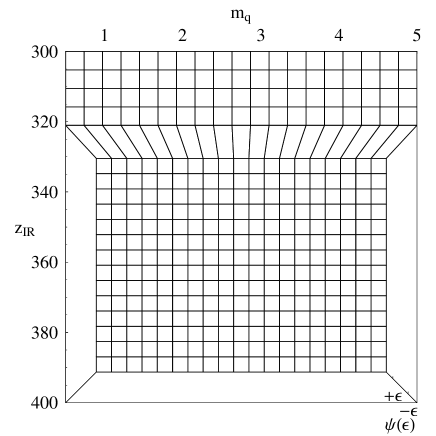
Figure 2: $\psi(\epsilon)$ as a function of $z_{IR}$ and $m_{q}$, showing the contour which corresponds to the physical boundary value for this field.

This result is as expected and tells us that the vector spectrum is determined largely through $\Lambda_{QCD}$ and not through $m_{q}$.

In order to fix the two parameters completely we now turn to the pion decay constant, calculated from the axial vector equation of motion with the pole in the propagator set to zero. Note that the axial vector equation of motion depends on the quark mass and condensate even neglecting the back reaction. The pion decay constant is given by:

$$f_{\pi}^{2}=\left.-\frac{1}{g_{5}^{2}}\frac{\partial_{z}A(q=0,z)}{z}\right|_{z=\epsilon}\ ,$$ (17)

Where the solution of the axial field $A$ is the solution of

$$48\pi^{2}zA(z)\left(\sigma z^{2}+m_{q}\right)^{2}+\left(3\sigma^{2}z^{6}+3\sigma m_{q}z^{4}+m_{q}^{2}z^{2}+12\right)A^{\prime}(z)-12zA^{\prime\prime}(z)=0\ .$$ (18)

This time we plot the value of $f_{\pi,mod}-f_{\pi,exp}$ as a function of the two free parameters, where $f_{\pi,mod}$ corresponds to the value calculated in this model and $f_{\pi,exp}$ corresponds to the experimental value. By combining this plot with the plot in figure 2 we can fix the values of the two free parameters precisely. These are found to be $m_{q}=2.4MeV$ and $\sigma=(323.5MeV)^{3}$.

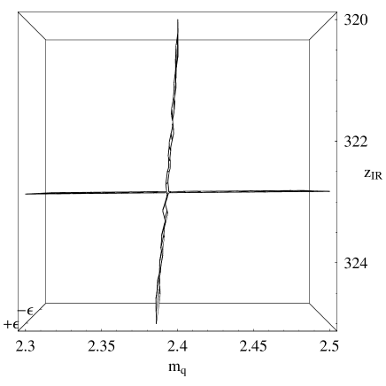
Figure 3: Intersection of the physical contours for both $f_{\pi}$ and $\psi(\epsilon)$ as a function of the two free parameters $z_{IR}$ and $m_{q}$. The point of intersection fixes the values to be used to calculate the observable predictions.

We fix the remaining free parameters of the theory from the intercept values of the two graphs and are now ready to calculate the remaining observable quantities, precisely as in [13]. The results of this analysis are given in table 1.

Observables	Measured Value	Non-back-reacted	Model I results	Model II results
	(MeV)	results (MeV (% error))	(MeV (% error))	(MeV (% error))
$m_{\pi}$	$139.6\pm 0.0004$	$139.6*$	$139.6*$	$139.6*$
$f_{\pi}$	$92.4\pm 0.35$	$92.4*$	$92.4*$	$92.4*$
$m_{\rho}$	$775.8\pm 0.5$	$775.8*$	$775.8*$	$769(0.9)$
$\sqrt{F_{\rho}}$	$345\pm 8$	$329(4.6)$	$334(3.2)$	$325.5(5.6)$
$m_{a_{1}}$	$1230\pm 40$	$1363(10.8)$	$1348(9.5)$	$1403(14)$
$\sqrt{F_{a_{1}}}$	$433\pm 13$	$486(12.2)$	$481(11)$	$514(18.8)$
$g_{\rho\pi\pi}$	$6.03\pm 0.07$	$4.44(26)$	$4.46(26)$	$4.49(25)$
rms error	-	15%	15%	16%

Table 1: Results of the non-back-reacted, non-singular back-reacted (Model I) and singular back-reacted (Model II) geometries. The percentage error is taken from the central value of the experimental measurement. $*$ indicates that this observable was used to fit the data.

We see that the effect of the back-reaction in this case is very small. We have shown that we can construct a phenomenologically consistent model, including back-reaction and obtain results in very close agreement with those without the back-reaction. The reason for this is simple. The effect of the back-reaction on the geometry will only become significant for energies of the order of $\sigma^{\frac{1}{3}}$. With the inclusion of the IR-brane, the geometry is cutoff just below the region where these effects would become significant and so the effects of the quark dynamics are shown to be negligible.

3.2 Model II

As stated in the previous section, it would be appealing to remove $z_{IR}$ as a free parameter and instead to generate it dynamically via a condensate. We examine one possible function with which we can do this and show that the results are promising.

Motivated by supergravity solutions we make a simple choice for $X$, of the form

$$X = \left(\frac{m_{q}z}{2}+\frac{1}{4}\log[\frac{1+\sigma z^{3}}{1-\sigma z^{3}}]\right){\mathbb{I}}_{2\times 2}\ ,$$

$$\lim_{z\rightarrow 0} \sim \ \left(\frac{m_{q}z}{2}+\frac{\sigma z^{3}}{2}\right){\mathbb{I}}_{2\times 2}\ ,$$ (19)

where the limiting behavior is for small $z$. The space is therefore cutoff at $z_{IR}=\frac{1}{\sigma^{\frac{1}{3}}}$.

Again we use the Gell-Mann-Oakes-Renner relation to constrain the relationship between $m_{q}$ and $\sigma$ leaving us with one free parameter which we can fix using the pion decay constant. The values are found to be $m_{q}=2.53$ $MeV$ and $\sigma=(320.3MeV)^{3}$.

We perform the same analysis using this model as we did in section 3.1. The results of this analysis are given in table 1. This singular back-reacted geometry gives good results and the important point is that the singular behavior does not destroy the original phenomenology. There are clearly many other sensible choices for $X$ which are both singular and give the correct UV behavior, however we show that with a sensible choice, such a model is phenomenologically consistent.

We can study the potential in the case of this singular back-reacted geometry and compare it to the original potential in the non-back-reacted case. This is shown in figure 4. We see that while the original potential is unbounded, the potential which classically gives us the singular field, $X$, gives a bounded potential with a minimum. The position of the minimum is a function of $m_{q}$ and $\sigma$ but its existence is not dependent on these values.

Figure 4: The potential in the five-dimensional action for both the non-back-reacted (dashed line) and back-reacted (full line), Model II, theories.

Though we treat the five-dimensional theory classically, from a quantum mechanical perspective, the potential in this singular, back-reacted geometry would have important consequences.

4 Discussion and Conclusion

In this paper we consider the back-reaction of the scalar on the metric in the holographic QCD model. In the hard wall model, the meson spectrum is generated by the IR brane. For pure AdS without the hard wall, the five-dimensional model is scale invariant and all the mesons are massless. Breaking the scale invariance is an essential mechanism in order to generate the meson spectrum. The mass gap $\Lambda_{QCD}$ is dual to the IR cut-off in this model. After considering the back-reaction, we find that the model still successfully describes the spectrum and decay constants of ground state mesons.

As for the resonances, in [22] it was shown that one can get linear confinement by including a quadratic dilaton $\Phi\sim z^{2}$ in the pure AdS background (see also [26] for a phenomenological treatment including a UV cutoff). The peculiar $z^{2}$ dependence of the dilaton is far from clear. If one considers the deformed AdS metric without introducing a dilaton:

$$ds^{2}={f(z)\over z^{2}}(dx_{\mu}dx^{\mu}-dz^{2}),$$

it can be shown that with $f(z)\sim(\cosh(az^{2})+b\sinh(az^{2}))^{4}$ and $a\neq 0$, one breaks scale invariance and gets linear confinement, even without the presence of the IR brane. However, the deformed AdS metric given by the back-reaction of the quark condensate is not compatible with this. Linear confinement can not be realized in this phenomenological model. From the non-polynomial form of $f(z)$, the first non-trivial term is quadratic in $z^{2}$. This suggests that a non-local dimension two condensate should be formed. In QCD, it has been investigated [27] that the non-zero value for the minimum of the vector potential condensate $A^{2}$, which is defined to be $\int d^{3}x\vec{A}^{2}(x)$ is possible. This dimension two condensate can be shown to be gauge invariant but non-local. Therefore, its effect should be relevant to linear confinement.

References

- [1] H. Fritzsch, M. Gell-Mann and H. Leutwyler, Phys. Lett. B 47, 365 (1973).
- [2] D. J. Gross and F. Wilczek, Phys. Rev. Lett. 30, 1343 (1973).
- [3] H. D. Politzer, Phys. Rev. Lett. 30, 1346 (1973).
- [4] Y. Nambu, Phys. Rev. Lett. 4 (1960) 380.
- [5] Y.B. Dai and Y.L. Wu, Eur.Phys.J. C39: S1 (2005).
- [6] G. ’t Hooft, Nucl. Phys. B 72, 461 (1974).
- [7] J. M. Maldacena, Adv. Theor. Math. Phys. 2, 231 (1998) [Int. J. Theor. Phys. 38, 1113 (1999)] [arXiv:hep-th/9711200].
- [8] S. S. Gubser, I. R. Klebanov and A. M. Polyakov, Phys. Lett. B 428, 105 (1998) [arXiv:hep-th/9802109].
- [9] E. Witten, Adv. Theor. Math. Phys. 2, 253 (1998) [arXiv:hep-th/9802150].
- [10] O. Aharony, A. B. Clark and A. Karch, Phys. Rev. D 74, 086006 (2006) [arXiv:hep-th/0608089].
- [11] L. von Smekal, R. Alkofer and A. Hauck, Phys. Rev. Lett. 79, 3591 (1997) [arXiv:hep-ph/9705242].
- [12] R. Alkofer, C. S. Fischer and F. J. Llanes-Estrada, Phys. Lett. B 611, 279 (2005) [arXiv:hep-th/0412330].
- [13] J. Erlich, E. Katz, D. T. Son and M. A. Stephanov, Phys. Rev. Lett. 95, 261602 (2005) [arXiv:hep-ph/0501128].
- [14] L. Da Rold and A. Pomarol, Nucl. Phys. B 721, 79 (2005) [arXiv:hep-ph/0501218].
- [15] J. Hirn and V. Sanz, JHEP 0512, 030 (2005) [arXiv:hep-ph/0507049].
- [16] S. J. Brodsky and G. F. de Teramond, AIP Conf. Proc. 814, 108 (2006) [arXiv:hep-ph/0510240].
- [17] L. Da Rold and A. Pomarol, JHEP 0601, 157 (2006) [arXiv:hep-ph/0510268].
- [18] K. Ghoroku, N. Maru, M. Tachibana and M. Yahiro, Phys. Lett. B 633, 602 (2006) [arXiv:hep-ph/0510334].
- [19] T. Hambye, B. Hassanain, J. March-Russell and M. Schvellinger, Phys. Rev. D 74, 026003 (2006) [arXiv:hep-ph/0512089].
- [20] J. Hirn, N. Rius and V. Sanz, Phys. Rev. D 73, 085005 (2006) [arXiv:hep-ph/0512240].
- [21] D. K. Hong and H. U. Yee, Phys. Rev. D 74, 015011 (2006) [arXiv:hep-ph/0602177].
- [22] A. Karch, E. Katz, D. T. Son and M. A. Stephanov, Phys. Rev. D 74, 015005 (2006) [arXiv:hep-ph/0602229].
- [23] N. Evans and T. Waterson, arXiv:hep-ph/0603249.
- [24] J. P. Shock and F. Wu, JHEP 0608, 023 (2006) [arXiv:hep-ph/0603142].
- [25] C. Csaki and M. Reece, arXiv:hep-ph/0608266.
- [26] N. Evans and A. Tedder, arXiv:hep-ph/0609112.
- [27] F. V. Gubarev, L. Stodolsky and V. I. Zakharov, Phys. Rev. Lett. 86, 2220 (2001) [arXiv:hep-ph/0010057].
- [28] D. Z. Freedman, S. S. Gubser, K. Pilch and N. P. Warner, Adv. Theor. Math. Phys. 3, 363 (1999) [arXiv:hep-th/9904017].