Neutrino Mixings and Leptonic CP Violation from CKM Matrix and Majorana Phases

Abstract

The high scale mixing unification hypothesis recently proposed by three of us (R. N. M., M. K. P. and G. R.) states that if at the seesaw scale, the quark and lepton mixing matrices are equal then for quasi-degenerate neutrinos, radiative corrections can lead to large solar and atmospheric mixings and small reactor angle at the weak scale in agreement with data. Evidence for quasi-degenerate neutrinos could, within this framework, be interpreted as being consistent with quark-lepton unification at high scale. In the current work, we extend this model to show that the hypothesis works quite successfully in the presence of CP violating phases (which were set to zero in the first paper). In the case where the PMNS matrix is identical to the CKM matrix at the seesaw scale, with a Dirac phase but no Majorana phase, the low energy Dirac phase is predicted to be ($\simeq 0.3^{\circ}$) and leptonic CP-violation parameter $J_{CP}\simeq(4-8)\times 10^{-5}$ and $\theta_{13}=3.5^{\circ}$. If on the other hand, the PMNS matrix is assumed to also have non-negligible Majorana phase(s) initially, the resulting theory damps radiative magnification phenomenon for a large range of parameters but nevertheless has enough parameter space to give the two necessary large neutrino mixing angles. In this case, one has $\theta_{13}=3.5^{\circ}-10^{\circ}$ and $|J_{CP}|$ as large as $0.02-0.04$ which are accessible to long baseline neutrino oscillation experiments.

hep-ph/0611225

HRI-P-06-11-004

I I Introduction

Grand unified theories ps ; georgi ; so10 ; rev with quark-lepton unification have often been used as key ingredients in attempts to understand the widely differing values of physical parameters describing particle interactions at low energies. In the context of SUSY GUTs, this approach can explain the experimentally measured values of the electro-weak mixing angle. The same models also lead to $b-\tau$ Yukawa unification buras which seems to be in rough agreement with observation or even $t-b-\tau$ Yukawa unification ananth which agree with observation for large values of $\tan\beta(=v_{u}/v_{d})$. It is then natural to explore whether there are other manifestations of quark lepton unification at low energies.

In a recent paper, three of us mpr1 discussed the possibility that weak interaction properties of quarks and leptons parameterized by very different flavor mixing matrices at low energies may become identical at high scales and provide another signature of quark–lepton unification. We found that if neutrinos are Majorana fermions with quasi-degenerate masses and with same CP, it could indeed happen i.e. starting with the CKM mixing matrix for neutrinos at the GUT-seesaw scale seesaw , as would be expected on the basis of quark–lepton unification ps , renormalization group evolution (RGE) to the weak scale leads to predictions for neutrino mixings in agreement with observations maltoni . Since small angles become larger, we have called this phenomenon radiative magnification and the interesting result is that the RGEs give two large mixings in the solar and atmospheric neutrino sectors while ultra smallness of $V_{ub}$ even after radiative magnification yields a small $\theta_{13}$ maintaining consistency with CHOOZ-Palo-Verde observations chooz . We then predicted $\sin\theta_{13}\leq 0.08-0.10$ which could be used to test the model mpr1 . We called this “high scale mixing unification” (HUM) hypothesis. The common mass of quasi-degenerate neutrinos required for HUM to work is in the range $0.15$ eV $\leq{\rm m}_{i}\leq 0.65$ eV. This falls in the appropriate range accessible to the currently planned experiments bb and overlaps with the values claimed by Heidelberg-Moscow ${\beta\beta}_{0\nu}$ experiment klapdor . It also overlaps the WMAP bound wmap and the range accessible to the KATRIN experiment katrin . It is also interesting to note that the radiative magnification mechanism with high-scale mixing unification works only for reasonably large values of $\tan\beta$ for which $t-b-\tau$ Yukawa unification takes place.

Furthermore, the HUM hypothesis provides an alternative way to understand the difficult problem of the diverse mixing patterns between quarks and leptons without relying on new mass textures for neutrinos or new family symmetries. This makes it interesting in its own right and in our opinion deserves further consideration.

Renormalization group effects on neutrino mass parameters over wide range of values have been discussed in a number of works using standard wett ; babu ; casas ; bdmp ; antusch1 ; antusch2 ; ellis or nonstandard xing parameterizations of the PMNS matrix; but our present and earlier results mpr1 ; mpr2 ; mpr3 are distinct in the following respects: (1) because of the underlying quark-lepton unification hypothesis, the input values of the three mixing angles are small at the GUT-seesaw scale and are identical to the corresponding CKM mixings mpr1 . The high scale input value of the Dirac phase in the PMNS matrix, which was set to zero in mpr1 and discussed in subsequent sections is also identical to the corresponding quantity in the CKM matrix. (2) The three light neutrinos are quasi-degenerate in mass. (3) The RH Majorana neutrino mass matrix is proportional to a unit matrix due to an $S_{4}$ mpr1 ; lee symmetry, which leads to quasi-degenerate light neutrinos through the type-II seesaw mechanism. (4) The heavy degenerate masses of RH neutrinos being very close to the the GUT-seesaw scale, large threshold corrections originating from non-degeneracy of RH neutrinos are absent in our case. In view of this, the model predictions are definite and can be tested more by planned neutrino experiments.

For the sake of simplicity, only CP conserving case was considered in mpr1 and all neutrino mass eigenstates were assumed to possess the same CP. Clearly, understanding CP phases is an integral part of understanding the flavor puzzle smir and it is therefore important to explore whether the “high scale mixing unification” hypothesis throws any light on this. The purpose of the present paper is to investigate this question.

Following the HUM hypothesis we identify the three mixing angles and the Dirac phase of the PMNS mixing matrix as those of the CKM mixing matrix at the GUT-seesaw scale while keeping the two Majorana phases as unknown. Whether exact quark-lepton symmetry at high scale permits nonzero values of the Majorana phases is a model dependent question; therefore, we consider two different cases: (i) when the high scale PMNS matrix with zero Majorana phases is identified with the CKM matrix; and (ii) when the PMNS matrix equals the product of the CKM matrix times a diagonal Majorana phase matrix. The diagonal-phase matrix may originate from the seesaw contribution to the neutrino mass.

We find that the radiative magnification of mixing angles are generally damped in the presence of Majorana phases and the degree of damping depends upon the values of these parameters. However in spite of this, the model has enough parameter space to magnify the mixing angles to be in agreement with the low-energy neutrino data starting from the CKM matrix at the GUT-seesaw scale; in this case, we find that $\theta_{13}$ and leptonic CP-violations are large enough to be measurable in long baseline neutrino oscillation experiments.

We also derive new analytic formulas for threshold corrections including Majorana phases which are generally valid in all models with quasi-degenerate neutrino masses. Out of a number of solutions which require  small threshold corrections to bring the solar neutrino mass squared difference in accord with experimental data as before, we find a new region in the parameter space where no such threshold corrections are necessary. We show how the the partial damping of magnification due to Majorana phases is utilized to obtain this new class of solutions.

This paper is organized as follows. In Sec.II we discuss the new boundary condition at the GUT seesaw scale and RGEs. In Sec.III we discuss input parameters at GUT-seesaw scale and some general criteria including the role played by Majorana phases in damping radiative magnification. In Sec.IV we present new analytic formulas showing how Majorana phases influence threshold corrections explicitly. Solutions to the RGEs and predictions in different cases are presented in Sec.V. In Sec.VI we discuss the new class of solutions without threshold corrections using damping property of Majorana phases. In Sec.VII we summarize the results briefly and state our conclusions.

II II  RG Equations and High Scale Boundary Condition

The starting point of our analysis is the assumption that there is an underlying gauge symmetry that unifies quarks and leptons and lead to the possibility that the CKM matrix for quarks and the PMNS matrix are equal. In mpr1 , we gave an example of this symmetry as $SU(2)_{L}\times SU(2)_{R}\times SU(4)_{C}$ times a discrete permutation family symmetry $S_{4}$. In this paper, we do not discuss any specific model but rather assume that such a symmetry exists implying the mixing unification at the seesaw scale. Given this hypothesis, the existence of the CKM phase would imply that the Dirac phase of the PMNS matrix at the GUT scale is the CKM phase. As far as the two Majorana phases of the PMNS matrix are concerned, they have no counterparts in the CKM matrix. However, due to seesaw mechanism, it is not implausible that the Majorana phases are also present at the high scale. We therefore study two possibilities: (i) setting the two Majorana phases to zero at the GUT-seesaw scale and examine the low energy behavior of the theory; (ii) treating the two phases as unknown parameters and see their effect.

The boundary condition for mixing angles at the seesaw scale is therefore given by :
$\mu=M_{R}$:

$$U_{PMNS}(M_{R})=V_{CKM}(M_{R})\times V_{D}(M_{R})$$ (1)

where $V_{CKM}$ is the RG-extrapolated CKM matrix for quark mixings from low energy data including its experimental value for the Dirac phase. The two unknown Majorana phases are provided through the diagonal matrix $V_{D}={\rm{diag}}(e^{i\alpha_{1}},e^{i\alpha_{2}},1)$. Thus, up to the presence of the diagonal phase matrix in eq.(1), this boundary condition establishes complete identity of the PMNS mixing matrix for leptons with the CKM mixing for quarks at the GUT-seesaw scale through the high scale mixing unification (HUM) hypothesis. Below the GUT-seesaw scale, however, there could be substantial differences between the two due to RG evolution effects and we parameterize the PMNS matrix as
$\mu<M_{R}$ :

$$U=\left[\begin{array}[]{ccc}c_{13}c_{12}&c_{13}s_{12}&s_{13}e^{-i\delta}\\ -c_{23}s_{12}-c_{12}s_{13}s_{23}e^{i\delta}&c_{12}c_{23}-s_{12}s_{13}s_{23}e^{i\delta}&c_{13}s_{23}\\ s_{12}s_{23}-c_{12}s_{13}c_{23}e^{i\delta}&-c_{12}s_{23}-c_{23}s_{13}s_{12}e^{i\delta}&c_{13}c_{23}\end{array}\right]\times{\rm{diag}}.\left(e^{i\alpha_{1}},e^{i\alpha_{2}},1\right)$$ (2)

where $c_{ij}=\cos\theta_{ij}$ and $s_{ij}=\sin\theta_{ij}(i,j=1,2,3$) and all the mixing angles and phases are now scale dependent. We have chosen the Majorana phases to be two times of that in usual parameterizations. This choice is made for the sake of convenience in computation. The values of the mixing angles at low energies will be obtained from RG evolution following the top-down approach under the boundary conditions,

$$\sin\theta_{12}^{0} \equiv \sin\theta_{12}(M_{R})_{PMNS}=\sin\theta_{12}(M_{R})_{CKM},$$

$$\sin\theta_{23}^{0} \equiv \sin\theta_{23}(M_{R})_{PMNS}=\sin\theta_{23}(M_{R})_{CKM},$$

$$\sin\theta_{13}^{0} \equiv \sin\theta_{13}(M_{R})_{PMNS}=\sin\theta_{13}(M_{R})_{CKM},$$

$$\delta^{0} \equiv \delta(M_{R})_{PMNS}=\delta(M_{R})_{CKM}$$ (3)

and the two Majorana phases at $\mu=M_{R}$ will be treated as unknown parameters, $\alpha_{1}^{0}$ and $\alpha_{2}^{0}$. The renormalization group equations (RGEs) for the neutrino mass matrix in the flavor basis were derived earlier and have been used to obtain a number of interesting conclusions especially for quasi-degenerate neutrinos babu ; bdmp in the flavor basis. As in the earlier case we find here more convenient to use RGEs directly for the mass eigenvalues and mixing angles including phases derived in the mass basis casas ; antusch2 . For the sake of RG solutions assume the three neutrino mass eigenvalues to be real and positive. The RGEs for the light neutrino mass eigenvalues can be written as

$${dm_{i}\over dt}=-2F_{\tau}(P_{i}+G_{i})m_{i}-m_{i}F_{u},\,\left(i=1,2,3\right)$$ (4)

The RGEs for mixing angles and phases are represented upto a good approximation for small $\theta_{13}$ which is actually the case through the following equations antusch2 ,

$$ds_{23}\over dt = \frac{F_{\tau}c_{23}\sin 2\theta_{23}}{2(m_{3}^{2}-m_{2}^{2})}\left[c_{12}^{2}(m_{3}^{2}+m_{2}^{2}+2m_{3}m_{2}\cos 2\alpha_{2})\right.$$ (5)

$$\left.+s_{12}^{2}(m_{3}^{2}+m_{1}^{2}+2m_{3}m_{1}\cos 2\alpha_{1})/(1+R)\right],$$

$$ds_{13}\over dt = -\frac{F_{\tau}c_{13}\sin 2\theta_{12}\sin 2\theta_{23}m_{3}}{2(m_{3}^{2}-m_{1}^{2})}\left[m_{1}\cos(2\alpha_{1}-\delta)\right.$$ (6)

$$\left.-(1+R)m_{2}\cos(2\alpha_{2}-\delta)-Rm_{3}\cos\delta\right],$$

$$ds_{12}\over dt = F_{\tau}c_{12}\sin 2\theta_{12}s_{23}^{2}\left[m_{1}^{2}+m_{2}^{2}+2m_{1}m_{2}\cos(2\alpha_{2}-2\alpha_{1})\right]/\left[2(m_{2}^{2}-m_{1}^{2})\right],$$ (7)

$${d\delta}\over{dt} = -\frac{F_{\tau}m_{3}\sin 2\theta_{12}\sin 2\theta_{23}}{2\theta_{13}(m_{3}^{2}-m_{1}^{2})}\times\left[m_{1}\sin(2\alpha_{1}-\delta)-(1+R)m_{2}\sin(2\alpha_{2}-\delta)+Rm_{3}\sin\delta\right]$$ (8)

$$-2F_{\tau}\left[\frac{m_{1}m_{2}s_{23}^{2}\sin(2\alpha_{1}-2\alpha_{2})}{(m_{2}^{2}-m_{1}^{2})}+m_{3}s_{12}^{2}\left(\frac{m_{1}\cos 2\theta_{23}\sin 2\alpha_{1}}{(m_{3}^{2}-m_{1}^{2})}+\frac{m_{2}c_{23}^{2}\sin(2\delta-2\alpha_{2})}{(m_{3}^{2}-m_{2}^{2})}\right)\right.$$

$$\left.+m_{3}c_{12}^{2}\left(\frac{m_{1}c_{23}^{2}\sin(2\delta-2\alpha_{1})}{(m_{3}^{2}-m_{1}^{2})}+\frac{m_{2}\cos 2\theta_{23}\sin 2\alpha_{2}}{(m_{3}^{2}-m_{2}^{2})}\right)\right],$$

$${d\alpha_{1}}\over{dt} = -2F_{\tau}\left[m_{3}\cos 2\theta_{23}\frac{(m_{1}s_{12}^{2}\sin 2\alpha_{1}+(1+R)m_{2}c_{12}^{2}\sin 2\alpha_{2})}{(m_{3}^{2}-m_{1}^{2})}\right.$$ (9)

$$\left.+\frac{m_{1}m_{2}c_{12}^{2}s_{23}^{2}\sin(2\alpha_{1}-2\alpha_{2})}{(m_{2}^{2}-m_{1}^{2})}\right],$$

$${d\alpha_{2}}\over{dt} = -2F_{\tau}\left[m_{3}\cos 2\theta_{23}\frac{(m_{1}s_{12}^{2}\sin 2\alpha_{1}+(1+R)m_{2}c_{12}^{2}\sin 2\alpha_{2})}{(m_{3}^{2}-m_{1}^{2})}\right.$$ (10)

$$\left.+\frac{m_{1}m_{2}s_{12}^{2}s_{23}^{2}\sin(2\alpha_{1}-2\alpha_{2})}{(m_{2}^{2}-m_{1}^{2})}\right]$$

where $R=(m_{2}^{2}-m_{1}^{2})/(m_{3}^{2}-m_{2}^{2})$, $P_{1}=s_{12}^{2}s_{23}^{2}$, $P_{2}=c_{12}^{2}s_{23}^{2}$, $P_{3}=c_{13}^{2}c_{23}^{2}$, $G_{3}=0$, but

$$G_{1} = -\frac{1}{2}s_{13}\sin 2\theta_{12}\sin 2\theta_{23}\cos\delta+s_{13}^{2}c_{12}^{2}c_{23}^{2},$$

$$G_{2} = \frac{1}{2}s_{13}\sin 2\theta_{12}\sin 2\theta_{23}\cos\delta+s_{13}^{2}s_{12}^{2}c_{23}^{2}$$ (11)

In the case of MSSM with $\mu\geq M_{\rm S}$,

$$F_{\tau} = {-h_{\tau}^{2}}/{\left(16\pi^{2}\cos^{2}\beta\right)},$$

$$F_{u} = \left(1\over{16\pi^{2}}\right)\left({6\over 5}g_{1}^{2}+6g_{2}^{2}-6{h_{t}^{2}\over\sin^{2}\beta}\right),$$ (12)

but, for $\mu\leq M_{\rm S}$,

$$F_{\tau} = {3h_{\tau}^{2}}/\left(32\pi^{2}\right),$$

$$F_{u} = \left(3g_{2}^{2}-2\lambda-6h_{t}^{2}\right)/\left(16\pi^{2}\right)$$ (13)

We would also need the CP-violation parameter defined through Jarlskog invariant jarlskog

$$J_{CP}~{}~{}=~{}~{}\frac{1}{8}\sin 2\theta_{12}\sin 2\theta_{23}\sin 2\theta_{13}\cos\theta_{13}\sin\delta$$ (14)

Since in the case of nonzero Majorana phases, the new phenomenon of damping of mixing angle magnification occurs, we first discuss this case, followed by the threshold corrections specific to this case before presenting the new results for the low energy predictions in both cases.

III III Magnification Damping by Majorana Phases and Input Parameters

In this section we discuss damping of radiative magnification caused by Majorana phases. While providing guidelines for the choice of input parameters we also point out some general features of the solutions in the context of the high scale mixing unification model. Throughout this paper all quantities with superscript zero indicate input parameters at the GUT-seesaw scale $M_{R}=10^{15}$ GeV.

For our calculation, we use the low energy data for the CKM matrix given by PDG pdg and we take into account the appropriate renormalization corrections to obtain their values at the GUT-seesaw scale. Due to the dominance of the top quark Yukawa coupling the one-loop renormalization corrections give falk ,

$${|V^{0}_{ub}|\over|V_{ub}|} = {|V^{0}_{cb}|\over|V_{cb}|}$$ (15)

$$\simeq exp\left[-{y_{top}^{2}\over 16\pi^{2}}\ln{M_{R}\over M_{Z}}\right]\simeq 0.83$$

while all other elements are almost unaffected. Using pdg ,

$$|V_{ub}| = 0.0037,|V_{cb}|=0.0413,$$

$$|V_{us}| = 0.2243,\delta=60^{\circ}\pm{14}^{\circ},$$ (16)

corresponding to

$$J_{CP}^{CKM}=2.89\times 10^{-5}$$ (17)

the input values for the CKM matrix at the GUT-seesaw scale are,

$$\sin\theta_{13}^{0}=0.0031,~{}~{}\sin\theta_{23}^{0}=0.034,~{}~{}\sin\theta_{12}^{0}=0.224,~{}~{}\delta^{0}=60^{\circ},$$ (18)

which yield

$$J_{CP}^{0}=2\times 10^{-5}$$ (19)

where we have fixed $~{}\delta^{0}$ and $J_{CP}^{0}$ at its central value after CKM extrapolation.

One point of utmost importance in this analysis is the nature of tuning needed in the neutrino mass eigenvalues which are inputs at the GUT seesaw scale. For quasi-degenerate neutrino masses having a common mass $m_{0}$ ,

$$(m_{2}-m_{1})={\Delta{m_{21}^{2}}\over 2m_{0}},~{}~{}(m_{3}-m_{2})={\Delta{m_{32}^{2}}\over 2m_{0}}$$ (20)

Using the experimental data from solar and atmospheric neutrino oscillations, $\Delta{m_{21}^{2}}=8\times 10^{-5}$ eV² and $\Delta{m_{32}^{2}}=2.4\times 10^{-3}$ eV² yields,

$$(m_{2}-m_{1})(eV) = 0.004,~{}~{}0.0002,~{}~{}0.0001,~{}~{}0.00004$$

$$(m_{3}-m_{2})(eV) = 0.12,~{}~{}0.006,~{}~{}0.003,~{}~{}0.0012$$

$$m_{0}(eV) = 0.01,~{}~{}0.2,~{}~{}0.4,~{}~{}1.0$$ (21)

This clearly suggests that if we confine ourselves to values of neutrino masses to be accessible to ongoing beta decay and double beta decay processes i.e. $m_{0}=0.1-1.0$ eV, fitting the experimental data on $\Delta m_{\odot}^{2}$ requires tuning between $m_{1}$ and $m_{2}$ at least up to fourth place of decimals while fitting the data on $\Delta m_{atm}^{2}$ needs tuning at least up to the third place of decimals between $m_{2}$ and $m_{3}$. The region of small common mass where the tuning improves by 1-2 orders is inaccessible to these experiments and also the RGEs do not succeed in achieving the desired magnification when $m_{0}<<0.1$ eV. We again emphasize the point noted in mpr1 that successful radiative magnification requires that $m_{0}\geq 0.1$ eV. Our idea can therefore be ruled out if there is no evidence for Majorana neutrino mass in the next round of neutrino double beta decay searches bb as well as, of course, by the measurement of $\theta_{13}$.

It is known that RGEs of neutrino mixing angles exhibit quasi-fixed points at low energies and these predicted quasi-fixed points are not in agreement with the observed experimental data casas . Exploiting the HUM hypothesis we have shown mpr1 ; mpr2 ; mpr3 that these quasi-fixed ponts can be avoided in supersymmetry throgh radiative magnification which is achieved by appropiate fine-tuning of quasi-degenerate neutrino mass eigen values and for larger values of $\tan\beta$. Such type of fine-tuning has been discussed in ref.mpr1 .

A useful general property of the RGEs with quasi-degenerate neutrinos is the following scaling behavior: for a set of solutions with masses $m_{i}$, mixings, phases, and mass squared differences $\Delta m_{ij}^{2}$, any other set of masses scaled to $\kappa m_{i}$ are also solutions with the same mixings and phases but with mass squared differences scaled to $\kappa^{2}\Delta m_{ij}^{2}$ where $\kappa$ is the common scaling factor for all mass eigenvalues. This property serves as a useful tool to derive other allowed solutions from one set of judiciously chosen numerical solutions to the RGEs.

From the structure of eq.(5)- eq.(10) it is clear that for a set of solutions $\alpha_{1},\alpha_{2},$ and $\delta$ , there exists another set of solutions $-\alpha_{1},-\alpha_{2},$ and $-\delta$ . The initial choice of input Majorana phases $(\alpha_{1}^{0},\alpha_{2}^{0})=(0,0),(\pi/2,\pi/2),(\pi,\pi)$ continue to retain their values to low energies up to a good approximation.

As noted in ref. mpr1 in the top down approach the RGEs for mass eigenvalues given in eq.(4) not only decrease the masses but they also decrease their differences such that at low energies $m_{i}\sim m_{j}$. The radiative magnification of the three mixing angles takes place for quasi-degenerate neutrinos because of smallness of the mass differences $m_{i}-m_{j}(i\neq j=1,2,3)$ that occurs  in the denominators of the RHS of RGEs for the mixing angles in eq.(5)- eq.(7). For the same reason large changes are also expected in the phases. During the course of RG evolution in the top-down approach $m_{i}\to m_{j}$ and the rate of magnification for mixing angles increases. Equivalently the solar and atmospheric mass differences decrease from their values at $\mu=M_{R}$ to approach their experimental values at $\mu=M_{Z}$ and the radiative magnification occurs for all the three mixing angles. While $\sin\theta_{12}$ and $\sin\theta_{23}$ attain their respective large values $\sin\theta_{13}$ remains small at low energies in spite of its magnification because its high scale starting value derived from the quark sector is much smaller($=|V^{0}_{ub}|$).

Note that since the input values for $\sin\theta_{12}^{0}$ , $\sin\theta_{23}^{0}$, and $\sin\theta_{13}^{0}$ are small with much smaller values for $\sin^{2}{\theta^{0}_{ij}}$ , but $\cos^{2}{\theta_{ij}^{0}}\simeq 1(i\neq j=1,2,3)$, it is clear from the RHS of eq.(5) that initially substantial contribution to the rate of magnification of $\sin\theta_{23}$ is caused by the dominant $c_{12}^{2}$ term, but $s_{12}^{2}$ term contributes only later during the course of evolution.

The following considerations hold when both the Majorana phases are small. In eq.(7) the coefficient on the RHS is proportional to $s_{12}s_{23}^{2}$ whose initial value is very small. Therefore the magnification of $\sin\theta_{12}$ requires very small difference between $m_{2}^{0}$ and $m_{1}^{0}$ compared to the difference $m_{3}^{0}-m_{2}^{0}$. On the other hand the dominant term in the RHS of eq.(5) is proportional to $s_{23}c_{23}^{2}c_{12}^{2}$ which is much larger near $\mu=M_{R}$ than the corresponding coefficient in eq.(7). The basic reason for this is essentially the smallness of CKM mixings near the GUT-seesaw scale which is totally different from the situations where initially there are large mixings antusch1 ; xing . Therefore in the HUM model radiative magnification of $\sin\theta_{23}$ can occur for larger mass difference between $m_{3}^{0}$ and $m_{2}^{0}$ compared to $m_{2}^{0}-m_{1}^{0}$ which is required for the magnification of $\sin\theta_{12}$ through eq.(7).

In the presence of finite values of Majorana phases the situation undergoes a quantitative change even if the smallness conditions in the initial mass differences are satisfied. In general damping in the magnification of the mixing angles $\theta_{12}$ and $\theta_{23}$ sets in whenever $\cos 2\alpha_{i}$ ($i=1,2$), or $\cos 2(\alpha_{1}-\alpha_{2})$ occurring in eq.(5) and eq.(7) deviate from $+1$.

To see the reason for magnification damping in a qualitative manner, note that the presence of Majorana phases is equivalent to multiplying the mass of the neutrino by that phase (i.e. $m_{0}e^{i\alpha}$). Now recall the well known case where for $\alpha_{1}-\alpha_{2}=(2n+1)\pi/2$ corresponding to the case of opposite CP-Parity of $\nu_{1}$ and $\nu_{2}$, magnification of $\theta_{12}$ is prevented. Similarly if $\alpha_{1}=\alpha_{2}=\pi/2$, the CP-Parity of $\nu_{3}$ is opposite to that of $\nu_{1}$ or $\nu_{2}$ and the mixing angle $\theta_{23}$ can not be magnified. In general values of $|\alpha_{1}|,|\alpha_{2}|$ different from $0$ or $\pi$ cause damping to the magnification of mixings, the damping being stronger for negative values of cosine functions occurring in the RHS of eq.(5) and eq.(7) . But as we find in spite of such dampings radiative magnification of the mixing angles can still be realized if these cosines have positive values $<1$ at lower scales. It is clear from eq.(5) that if $\alpha_{2}=\alpha_{1}=\pi/2$ the magnification of $\sin\theta_{23}$ can not occur even though the smallness condition on the mass difference $m_{3}^{0}-m_{2}^{0}$ is satisfied. If $\alpha_{2}\simeq\pi/2$ this magnification is badly affected. In fact even if $\alpha_{1}^{0}$ is small, but if $\alpha_{2}>{\pi\over 4}$ the dominant magnifying term in eq.(5) would start decreasing and it would need still smaller value of the initial mass difference $m_{3}^{0}-m_{2}^{0}$ to achieve magnification. As a result this region of Majorana phases would be restricted by the low energy data on $\Delta{m_{32}^{2}}$ since the latter is proportional to the mass difference $(m_{3}-m_{2})$.

From eq.(7) we see that no magnification can occur for $\sin\theta_{12}$ if $|\alpha_{2}-\alpha_{1}|\simeq\pi/2$ which can be satisfied for $\alpha_{2}\simeq 0$, $\alpha_{1}\simeq\pi/2$ or for $\alpha_{1}\simeq 0$, $\alpha_{2}\simeq\pi/2$. Eq.(5) and eq.(7) permit magnifications of $\sin\theta_{23}$ and $\sin\theta_{12}$ for small values of the Majorana phases $\alpha_{1},\alpha_{2}<{\pi\over 4}$ . Also when $\alpha_{2}$ is small, magnification is allowed for all values of $\alpha_{1}=0-\pi$ except in the region $\alpha_{1}\simeq{\pi\over 2}$ where the magnification of the solar mixing angle is strongly damped out for similar choice of the mass difference $m_{2}^{0}-m_{1}^{0}$ for which magnification takes place in other cases.

When $\alpha_{1}\simeq\alpha_{2}\simeq 0$, it is clear from eq.(8) that ${d\delta\over dt}$ is directly proportional to $\sin\delta$ and the RG solution for the leptonic Dirac phase approaches $\delta\to 0$ as $\mu\to M_{Z}$. A general consequence of the RGEs for the Majorana phases is that if we start with the initial condition $\alpha_{1}^{0}=\alpha_{2}^{0}$ at the GUT-seesaw scale, they would obtain equal values during the course of evolution antusch2 . Therefore if we start with vanishing Majorana phases at the GUT-seesaw scale they continue to remain zero at low energies.

Even though certain input values of Majorana phases might appear to be affecting magnification of mixings at high scales, their role to cause damping becomes different at lower scales as the supplied phases change by RG evolution. Particularly the damping becomes most severe for the choice $\alpha_{1}^{0}\simeq\alpha_{2}^{0}={\pi/2}$ since these phases which damp out magnification of both the mixing angles to start with remain almost unaltered during the course of evolution.

Although certain choices of input values of Majorana phases can cause partial or total damping of magnification of mixing angles, moderate damping with other choices can be utilised to obtain smaller mass squared differences at low energies. Exploiting this mechanism we show in Sec.VI how we identify a region in parameter space where $\Delta{m_{21}^{2}}$ needs no threshold corrections to be in agreement with the experimental data. On the other hand with MSSM spectrum below the GUT-seesaw scale, as the super-partner masses do not appear to be very close to $\mu=M_{Z}$, small threshold corrections to mass squared differences due to super-partners are quite natural in any such model containing the MSSM. In the next section we present derivation of new formulas showing how Majorana phases also affect threshold corrections in all models having quasi-degenerate neutrino masses.

IV IV Threshold Effects with Majorana Phases

With MSSM as the effective theory below the GUT-seesaw scale and non-degenerate super-partner masses new threshold corrections at $\mu=M_{Z}$ arise in any model having quasi-degenerate neutrino masses chun . They have been derived  in the quasi-degenerate case in the limit $\theta_{13}\to 0$ and $\theta_{23}\to\pi/4$ but without phases mpr2 . Following the same procedure and noting that the mixing matrix elements $U_{\alpha i},(i=1,2)$ now contain Majorana phases, we obtain the new generalized analytic formulas which are valid in all models with quasi-degenerate spectrum,

$$(\Delta m_{21}^{2})_{th} = 4\rm m^{2}\left[\left(s_{12}^{2}\cos 2\alpha_{2}-c_{12}^{2}\cos 2\alpha_{1}\right)T_{e}+\left(c_{12}^{2}\cos 2\alpha_{2}-s_{12}^{2}\cos 2\alpha_{1}\right){(T_{\mu}+T_{\tau})\over 2}\right],$$

$$(\Delta m_{31}^{2})_{th} = 4\rm m^{2}\left[-T_{e}c_{12}^{2}\cos 2\alpha_{1}+\left(1-s_{12}^{2}\cos 2\alpha_{1}\right){(T_{\mu}+T_{\tau})\over 2}\right],$$

$$(\Delta m_{32}^{2})_{th} = 4\rm m^{2}\left[-T_{e}s_{12}^{2}\cos 2\alpha_{2}+\left(1-c_{12}^{2}\cos 2\alpha_{2}\right){(T_{\mu}+T_{\tau})\over 2}\right]$$ (22)

Here $m$ represents the common mass of quasi-degenerate neutrinos. The functions $T_{\alpha},(\alpha=e,\mu,\tau)$ are one loop factors obtained by evaluation of corresponding Feynman diagrams, especially with wino and charged slepton exchanges chun .

$$T_{\alpha}=(g^{2}/{32\pi^{2}})[(x_{\mu}^{2}-x_{\alpha}^{2})/(y_{\mu}y_{\alpha})+((y_{\alpha}^{2}-1)/y_{\alpha}^{2})ln(x_{\alpha}^{2})-((y_{\mu}^{2}-1)/y_{\mu}^{2})ln(x_{\mu}^{2})]$$ (23)

where $y_{\alpha}=1-x_{\alpha}^{2}$, $x_{\alpha}=M_{\alpha}/M_{\tilde{w}}$, $M_{\alpha}=$ charged slepton mass, and $M_{\tilde{w}}=$ wino mass. and the loop-factor has been defined to give $T_{\mu}=0$ without any loss of generality. Depending upon the allowed low energy values of the Majorana phases the threshold corrections may vary for given values of the super-partner masses. In particular when $\alpha_{1}=\alpha_{2}=0,n\pi$, these generalized formulas reduce to those obtained in ref. mpr2 ,

$$(\Delta m_{21}^{2})_{th} = 4\rm m^{2}\cos^{2}\theta_{12}[-T_{e}+(T_{\mu}+T_{\tau})/2],$$

$$(\Delta m_{32}^{2})_{th} = 4\rm m^{2}\sin^{2}\theta_{12}[-T_{e}+(T_{\mu}+T_{\tau})/2],$$

$$(\Delta m_{31}^{2})_{th} = 4\rm m^{2}\cos^{2}\theta_{12}[-T_{e}+(T_{\mu}+T_{\tau})/2]$$ (24)

Including threshold corrections along with the RG-evolution effects the mass squared differences are evaluated using

$$\Delta m_{ij}^{2}=(\Delta m_{ij}^{2})_{\rm RG}+(\Delta m_{ij}^{2})_{\rm th}$$ (25)

where the RG-evolution effects from $M_{\rm R}$ to $M_{\rm Z}$ are computed using the procedure discussed in Sec.II - Sec.III. For several allowed mass ratios, $M_{\tilde{\rm e}}/M_{{\tilde{\mu}},{\tilde{\tau}}}\simeq 1.4-2.8$, consistent with an inverted hierarchy in the charged-slepton sector we find that the RG and the threshold corrections together are in good agreement with the available experimental data as discussed in Sec.V and in Table I. Small changes in the mixing angles due to threshold corrections in the masses are easily compensated by very small changes in the input mass eigenvalues leading to predictions given in Table.I in the next section. In Sec.VI we also present solutions without any threshold corrections.

V V Low Energy Predictions in the Leptonic Sector

In this section we present the predictions of our model as solutions of RGEs with Dirac and Majorana phases. As explained in ref. mpr1 at first we follow bottom up approach to obtain information on the Yukawa and gauge couplings at the GUT-seesaw scale to serve as inputs in the top down approach. The extrapolated values of the gauge and the Yukawa couplings for $\tan\beta=55$ at $M_{R}=10^{15}$ GeV are: $g_{1}^{0}=0.6683,g_{2}^{0}=0.6964,g_{3}^{0}=0.7247,h_{\rm{top}}^{0}=0.8186,h_{b}^{0}=0.6437$, and $h_{\tau}^{0}=0.7105$. We choose the high seesaw scale $M_{R}=10^{15}$ GeV where the mixing angles and the Dirac phase are those given in eq.(18). We use high scale input mass eigenvalues as discussed above. Using solutions of RGEs combined with such threshold corrections discussed in Sec.IV in the appropriate cases we treat the results as acceptable if they are within $4\sigma$ limit of the available data from neutrino oscillation experiments although a substantial part of our solutions in the parameter space are either in the best fit region or within $2\sigma$ to $3\sigma$ limits maltoni ,

$$\Delta{m_{21}^{2}} = (6.8-9.3)\times 10^{-5}eV^{2},$$

$$\Delta{m_{31}^{2}} = (1.8-3.5)\times 10^{-3}eV^{2},$$

$$\sin^{2}\theta_{12} = 0.22-0.44,$$

$$\sin^{2}\theta_{23} = 0.31-0.71,$$

$$\sin^{2}\theta_{13} \leq 0.058$$ (26)

Since the other factor occurring in $J_{CP}$ is almost determined from the solar and atmospheric mixing angles, $(\sin 2\theta_{12}\sin 2\theta_{23})/8\simeq 0.1$ the model dependent quantity $|\rm{Im}U_{e3}|\simeq O(0.1)$ if the prediction is to be verified by long base line neutrino oscillation experiments in near future. The predictions of $\theta_{13}$ and $\delta$ vary from model to model. In the present case the initial value of $V^{0}_{ub}$ including the Dirac phase $\delta^{0}$ and the input values of the Majorana phases determine $\theta_{13}$ and $\delta$ at low energies by RG evolution while matching the experimental values of the other two neutrino mixing angles by radiative magnification. We find that in the presence of Majorana phases our model predicts values of $|\rm{Im}U_{e3}|$ contributing to $|J_{CP}|\simeq O(10^{-2})$ accessible for measurement by neutrino oscillation experiments.

As discussed in Sec.III the most flexible choice in the parameter space for which radiative magnification of mixings takes place easily is with $\alpha_{2}^{0}<45^{0}$ or $\alpha_{2}^{0}>135^{0}$ and varying $\alpha_{1}^{0}$. We present below details of results obtained on mass squared differences, mixing angles, low energy values of different phases and the CP-violation parameter. In all cases the Dirac phase of the PMNS matrix has been fixed at $60^{\circ}$ at the GUT-seesaw scale. The other class of solutions obtained using the magnification damping criteria and which needs no threshold corrections due to super-partner masses will be presented in Sec.VI.

V.1 V.1 Low Energy Predictions for $\theta_{13}$ and Majorana Phases

Since Majorana phases do not occur in eq.(4) and Dirac phase dependent terms are very small, the evolution of mass eigen values are almost the same as reported earlier mpr1 . They decrease from their high scale input values and tend to converge towards one another narrowing their differences until agreement with experimental data on $\Delta{m_{31}^{2}}$ and $\Delta{m_{21}^{2}}$ are obtained with or without small threshold corrections. Even in the presence of phases the radiative magnification to bi- large neutrino mixings maintain the similar correlations as before: Decreasing differences between the mass eigenvalues is accompanied by increasing magnification of mixing angles and finally their largest predicted values are obtained at $\mu=M_{Z}-M_{S}$ where $M_{S}=1$ TeV is the SUSY scale. For example with the input value of one Majorana phase set to a vanishing value at the GUT-seesaw scale ($\alpha_{2}^{0}=0.0$), the radiative magnification to bi-large neutrino mixings takes place for all values of the other Majorana phase $\alpha_{1}^{0}=0-\pi$ except at $\alpha_{1}^{0}\simeq{\pi\over 2}$ where almost total damping occurs for the magnification of $\sin\theta_{12}$.

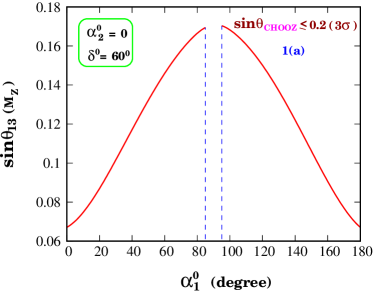
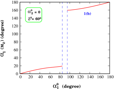
Figure 1: 1(a). Prediction of CHOOZ angle as function of input Majorana phase $\alpha_{1}^{0}$ at the GUT-seesaw scale for $\alpha_{2}^{0}=0$. The vertical dashed lines define the total damping region for $\sin\theta_{12}$ magnification corresponding to $\alpha_{1}^{0}=90^{\circ}\pm 5^{\circ}$. 1(b). RGE-solution for $\alpha_{1}$ at low energies as a function of the input phase at the GUT-seesaw scale.

Fig. 1(a) shows predicted variation of $\sin\theta_{13}$ at low energies as a function of $\alpha_{1}^{0}$. It is clear that starting from $\theta_{13}=3.5^{\circ}$ at $\alpha_{1}^{0}=0$ the value of $\theta_{13}$ continuously increases reaching a maximal value at $\alpha_{1}^{0}\simeq 85^{\circ}$. Again after the disfavored region at $\alpha_{1}^{0}\simeq 90^{\circ}\pm 5^{\circ}$, it decreases from its maximal value continuously in the second quadrant till it reaches low value at $\alpha_{1}^{0}\simeq\pi$. The predicted range of $\theta_{13}\simeq 3.5^{\circ}-10^{\circ}$ and the maximum predicted value is nearly $25\%$ smaller than the current $4\sigma$ upper bound. This prediction is new and covers a wider range compared to that found in ref. mpr1 where the PMNS matrix had no phase.

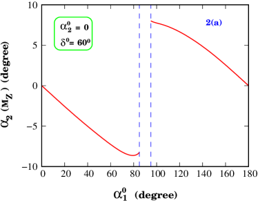
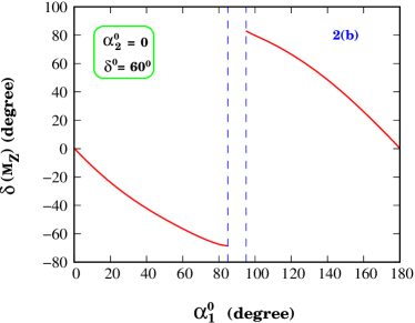
Figure 2: 2(a). RGE-solution for $\alpha_{2}$ at low energies as a function of input $\alpha_{1}^{0}$ at the GUT-seesaw scale. 2(b). RGE-solution for leptonic Dirac phase at low energies as a function of $\alpha_{1}^{0}$.

The low energy values of Majorana phases corresponding to the input values of $\alpha_{1}^{0}$ are shown in Fig.1(b)and Fig.2(a). We note from Fig. 1(b) that corresponding to input $\alpha_{2}^{0}=0.0$ the Majorana phase $\alpha_{1}(M_{Z})$ at low energies increases from $0^{\circ}$ to $20^{\circ}$ when the input $\alpha_{1}^{0}$ varies from $0^{\circ}$ to $85^{\circ}$ in the first quadrant but $\alpha_{1}(M_{Z})$ varies from $155^{\circ}$ to $180^{\circ}$ when $\alpha_{1}^{0}$ varies in the second quadrant. From Fig. 2(a) we find that though the value of $\alpha_{2}^{0}=0$ at the GUT-seesaw scale, its value at low energies is non-vanishing with $\alpha_{2}(M_{Z})\simeq 0^{\circ}$ to $-8^{\circ}$ when $\alpha_{1}^{0}$ varies over the first quadrant, but $\alpha_{2}(M_{Z})=8^{\circ}$ to $0^{\circ}$ when $\alpha_{1}^{0}$ is in the second quadrant.

V.2 V.2 Predictions for Dirac Phase and Leptonic CP Violation

Two interesting features of the model are the unification of the CKM Dirac phase with the PMNS Dirac phase and also the unification of quark CP-violation with the leptonic CP-violation at the GUT-seesaw scale. We summarize low energy predictions of leptonic CP-violation in two different cases: (i) When Majorana phases are absent in the PMNS matrix at high scales, (ii) When the high scale PMNS matrix contains Majorana phases as unknown parameters.

V.2.A  CP-Violation without Majorana Phases

When the two Majorana phases are set to zero at the GUT see saw scale, the PMNS matrix unifies with the CKM matrix including its Dirac phase. As a consequence of the RGEs in the top down approach in the $\theta_{13}\to 0$ limit, the Dirac phase rapidly decreases to approach its trivial fixed point $\delta\to 0$. Both the Majorana phases also continue to maintain their vanishing values in this limiting case at all energies below the GUT-seesaw scale and we obtain

$$\delta \simeq 0.3^{\circ}-1^{\circ},~{}~{}\theta_{13}\simeq 3.5^{\circ}-4.5^{\circ},$$

$$J_{CP} \simeq (5-7.6)\times 10^{-5}$$ (27)

Thus, without initial Majorana phases, the CP-violation parameter is a few times larger than the corresponding low energy value in the CKM matrix even though the low energy value of the Dirac phase is suppressed by a factor $\simeq 10^{-2}$ than the corresponding CKM Dirac phase. This occurs due to the predicted value of the CHOOZ angle which is nearly $20$ times larger than its counterpart in the quark sector ($|V_{ub}|$) at low energies.

V.2.B  CP-Violation with Majorana Phases

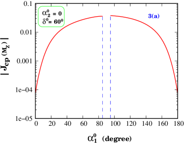
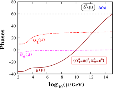
Figure 3: 3(a).Prediction for the leptonic CP-violation parameter at low energies as a function of input Majorana phase $\alpha_{1}^{0}$ at the GUT-seesaw scale. 3(b). Evolution of the leptonic Dirac phase and Majorana phases from the GUT-seesaw scale down to low energies. The horizontal dotted line shows the constancy of the CKM Dirac phase with unification point at the GUT-seesaw scale.

The predictions on the leptonic Dirac phase and CP-violation parameter change substantially at low energies in the presence of finite input values of Majorana phase(s) at the GUT-seesaw scale. The variation of predicted leptonic Dirac phase $\delta$ and the leptonic CP-violation parameter $J_{CP}$ at low energies with the input Majorana phase $\alpha_{1}^{0}$ are shown in Fig. 2(b) and Fig. 3(a), respectively. It is clear from Fig. 2(b) that the leptonic Dirac phase varies from $0.3^{0}$ to $-70^{\circ}$ when $\alpha_{1}^{0}$ is in the first quadrant, then it becomes positive and varies from $80^{\circ}$ to $0.3^{\circ}$ when $\alpha_{1}^{0}$ is in the second quadrant. The variation of the leptonic CP-violation parameter is correlated with the variation of the leptonic Dirac phase with $\alpha_{1}^{0}$. In Fig. 3(a) the low-energy values of $J_{CP}(M_{Z})$ in the first(second) quadrant are negative(positive). It is clear from Fig. 3(a) that $J_{CP}(M_{Z})$ varies from $-7\times 10^{-5}$ to $-0.03$ when $\alpha_{1}^{0}$ is in the first quadrant , but then it changes sign and varies from $0.038$ to $7\times 10^{-5}$ when $\alpha_{1}^{0}$ is in the second quadrant.

The evolution of Dirac and Majorana phases are shown in Fig. 3(b) corresponding to the input values $\alpha_{1}^{0}=30^{\circ},\alpha_{2}^{0}=0.0$. While $\alpha_{1}(\mu)$ is found to decrease by nearly $50\%$, a nonzero value for $\alpha_{2}(\mu)$ is found to have been generated at $\mu=M_{Z}$ from its vanishing boundary value at the GUT-seesaw scale. The solid(dotted) line in Fig. 3(b) represents the evolution of the leptonic(CKM) Dirac phase with unification at the GUT-seesaw scale. While the CKM Dirac phase remains constant the leptonic Dirac phase is found to evolve to nearly $-35^{\circ}$ at low energies starting from its unified value of $60^{\circ}$ at the GUT-seesaw scale.

One of the most interesting and novel outcome of this analysis is the prediction of the leptonic CP-violation starting from the corresponding baryonic CP-violation as embodied in the CKM matrix as shown in Fig. 4(a) and Fig. 4(b) where the dotted line represents very slow evolution of the CKM CP-violation parameter. While in Fig. 4(a) we present positive values of the parameter in Fig. 4(b) we present negative values depending upon the initial choice of Majorana phases. The dot-dashed line in Fig. 4(a) represents the evolution of the leptonic CP-violation parameter starting from its unified CKM value of  $2\times 10^{-5}$. In the absence of any Majorana phase the radiative magnification caused due to quasi-degenerate neutrinos has enhanced it by nearly a factor of only $\simeq 3.5$ making the low energy prediction $J_{CP}=7.6\times 10^{-5}$.

In the presence of non-vanishing Majorana phase(s), the parameter evolves to much larger values at low energies as shown by the dashed and solid lines in Fig. 4(a) corresponding to $J_{CP}(M_{Z})\simeq 0.01-0.03$.  In Fig. 4(b) the negative values of the parameter at low energies are in the range $J_{CP}(M_{Z})\simeq-0.013$ to $-0.036$. It is clear from these two figures that major part of magnification of $|J_{CP}|$ occurs in the region $\mu=10^{5}$ GeV to $10^{3}$ GeV. We note that the continued smallness of the CP-violation parameter at high scales for $\mu=10^{7}$ GeV to $10^{15}$ GeV might have some cosmological significance. Although these predicted values of the re-phasing invariant parameter, $|J_{CP}(M_{Z})|\simeq 0.02-0.04$ at low energies that relates only the Dirac phase, are accessible for measurement by long baseline neutrino oscillation experiments, we have also estimated the model predictions on the two other invariants relating to Majorana phases jarlskog ; picariello for the sake of completeness,

$$S_{1} = Im\left(U_{\nu_{e}\nu_{1}}U_{\nu_{e}\nu_{3}}^{*}\right)=\frac{1}{2}\sin 2\theta_{13}\cos\theta_{12}\sin(\alpha_{1}+\delta),$$

$$S_{2} = Im\left(U_{\nu_{e}\nu_{2}}U_{\nu_{e}\nu_{3}}^{*}\right)=\frac{1}{2}\sin 2\theta_{13}\sin\theta_{12}\sin(\alpha_{2}+\delta)$$

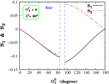
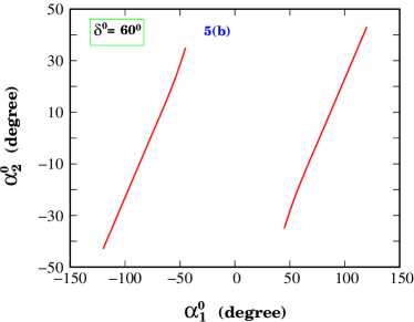
Figure 5: 5(a). Predictions of the two invariants relating to Majorana phases as defined in Sec.V.2.B in the text. 5(b).  Two branches of the parameter space defined for no threshold corrections through the magnification damping condition ${\rm C}os~{}2(\alpha_{1}^{0}-\alpha_{2}^{0})=-0.9$ at the GUT-seesaw scale.

The predicted values of these two parameters are shown in Fig. 5(a) as a function of the input Majorana phase $\alpha_{1}^{0}$ while $\alpha_{2}^{0}=0$. We find that starting from $S_{1}\simeq S_{2}\simeq 10^{-4}$ these parameters are bounded by $|S_{1}|\leq 0.1$ and $|S_{2}|\leq 0.14$ for this choice of Majorana phases. If in future, experiments on neutrinoless double beta decay determine one of the two Majorana phases, then with possible information on $\theta_{13}$ and the leptonic Dirac phase from neutrino oscillation experiments, the predictions on one of these parameters might be tested.

V.3 V.3 Neutrinoless Double Beta Decay, Tritium Beta Decay and Cosmological Bound

The search for neutrinoless-double beta decay by Heidelberg-Moscow experiment has obtained the upper limit,

$$<m_{ee}><(0.33-1.35)~{}{\rm{eV}}\\$$ (28)

which overlaps the range that will be covered in the planned experiments cremo . Similarly the current upper bound on the kinematical mass from Tritium beta decay is $<m_{e}><2.2$ eV . But the KATRIN experiment is expected to probe $<m_{e}>\geq 0.2$ eV and if positive it would prove that the neutrino masses are quasi-degenerate rnm . Using

$$<m_{ee}> = |m_{1}c_{12}^{2}c_{13}^{2}+m_{2}s_{12}^{2}c_{13}^{2}e^{-2i(\alpha_{2}-\alpha_{1})}+m_{3}s_{13}^{2}e^{2i(\delta+\alpha_{1})}|,$$

$$<m_{e}> = \left[m_{1}^{2}c_{12}^{2}c_{13}^{2}+m_{2}^{2}s_{12}^{2}c_{13}^{2}+m_{3}^{2}s_{13}^{2}\right]^{1/2}$$ (29)

we have evaluated these effective masses using our solutions for mass eigen values, mixing angles and Majorana and Dirac phases at low energies. Some of our solutions including small threshold corrections estimated using the formulas given in eq.(22) - eq.(23) are presented in Table I while others without the necessity of threshold corrections are discussed in Sec. VI and presented in Table II. It is clear that not only the model predictions are in good agreement with the current data from neutrino oscillation experiments, but also the mass parameters are in the interesting range accessible to the Heidelberg Moscow experiment on double beta decay and the KATRIN experiment on beta decay. At this stage we emphasize that since the super-partner masses may be naturally in the range of $150$ GeV $-1$ TeV, small threshold corrections in the MSSM near the electroweak scale or even at $\mu=M_{S}=1$ TeV are quite natural.

Taking into account the allowed range of positive mass eigenvalues this analysis predicts the sum of three quasi-degenerate neutrino masses to be in the range $\Sigma_{i}m_{i}=(0.7-1.2)$ eV. Recent data from WMAP gives the bound on the sum of the three neutrino masses in the  range $(0.7-2.1)$ eV depending upon what values one chooses for the priors. The cosmological bound may be as large as $3$ eV wmap ; fukugita . In this context it is interesting to note that the presence of Dark Energy may have strong impact on cosmological bounds on neutrino masses taking the lowest value of WMAP bound on the sum without priors from $0.7$ eV to $1.4$ eV hannestad .

We find that the values of quasi-degenerate neutrino masses predicted in the model are consistent with the current cosmological bounds.

VI VI Parameter Space for No Threshold Correction

As pointed out earlier mpr1 ; mpr2 and utilized in Sec. IV and Table I the low energy solutions for $\Delta{m_{21}^{2}}$ in the presence or absence of Majorana phases need small threshold corrections due to possible spreading of sfermion masses above the electroweak scale to bring $\Delta{m_{21}^{2}}$ to be in agreement with the experimental data. Of course these corrections are quite natural and must be included in any SUSY model of quasi-degenerate neutrino masses. In the present case a class of our solutions for $\Delta{m_{21}^{2}}$ need such small threshold corrections which are readily computed as discussed in mpr2 ; chun .

In this Section we find an interesting new aspect of the radiative magnification mechanism in the presence of Majorana phases: i.e. there is a region in the parameter space which needs no threshold corrections for the mass squared differences to be in agreement with observations. In terms of initial values of the Majorana phases we find that this region of parameter space is described to a very good approximation by the two branches of the curve presented in Fig. 4(b). This curve is described by the equation,

$${\rm C}os~{}2(\alpha_{1}^{0}-\alpha_{2}^{0}) = {\rm{Const}}.$$

$$\rm{Const}. \simeq -0.9$$ (30)

These solutions without threshold corrections and with Majorana phases consistent with eq.(30) are given in Table II. It is clear that in this case the predictions for the reactor angle $\theta_{13}$, the Dirac phase and the CP-violating parameter are accessible to long baseline experiments while the effective neutrino mass parameter is within the range to be probed in neutrinoless double beta decay experiments as well as the KATRIN experiment. Further the sum of the three neutrino masses is also consistent with the cosmological bound including those from WMAP.

It is interesting to examine the physical origin behind such solutions. At first we note that eq.(30) looks very much like a strong damping condition on the radiative magnification of $\sin\theta_{12}$ as discussed in Sec.III. But, in reality, the values of Majorana phases change from their high-scale boundary values and while the major part of magnification takes place at lower scales, ${\rm C}os~{}2(\alpha_{1}(\mu)-\alpha_{2}(\mu))$ becomes positive and remains in the moderate damping region. In fact we have found from low energy values obtained from RG evolution that ${\rm C}os~{}2(\alpha_{1}(M_{Z})-\alpha_{2}(M_{Z}))=0.49-0.58$ as shown in Table. II.

Having shown that this cosine function is in the moderate damping region it then follows from eq.(7) that the radiative magnification of $\sin\theta_{12}$ in the presence of such moderate damping requires smaller mass difference between $m_{2}$ and $m_{1}$ than the corresponding case with weaker damping. This then leads to solutions to RGEs with smaller $\Delta{m_{21}^{2}}$ which needs no threshold corrections.

VII VII Conclusion

In conclusion, we have extended the results of the high scale mixing unification (HUM) hypothesis discussed in mpr1 by including the effects of the CP phases. We have considered the cases with and without the Majorana phases. While the mixing unification hypothesis predicts the Dirac phase to be equal to the CKM phase, it leaves the Majorana phases arbitrary since they have no quark counterpart and will most likely arise from the right handed neutrino sector. For both cases, we find consistent quasi-degenerate neutrino mass patterns that lead to desired amount of radiative magnification of the mixings in agreement with data. The predictions of the model are as follows: the common mass of the neutrinos must be larger than $0.1$ eV; the values of $\theta_{13}$ and CP phases in the lepton sector are also predicted at low energies. In the case without the Majorana phase, the low energy CP violating effect is small with $J_{CP}\simeq 7.6\times 10^{-5}$, whereas for the case with Majorana phases, $J_{CP}$ can be as large as $0.04$. An interesting phenomenon in the latter case is the damping of radiative magnification of neutrino mixing angles which constrains the Majorana phases to remain in a certain range for the model to explains the two large neutrino mixing angles. In this case, we predict a wider range of $\theta_{13}$ from $3.5^{\circ}-10^{\circ}$. The larger ranges for both $\theta_{13}$ and $J_{CP}$ are accessible to measurements by long baseline neutrino oscillation experiments.

The quasi-degenerate neutrino masses required to achieve desired radiative magnification, are consistent with the current cosmological bounds including those from WMAP. They are also accessible to the ongoing laboratory experiments on neutrinoless double beta decay and overlaps the range of KATRIN experiment for beta decay.

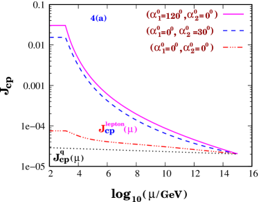
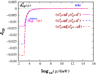
Figure 4: 4(a). Evolution of the leptonic CP-violation parameter from the GUT-seesaw scale to low energies for different input values of Majorana phases and for positive values of $J_{CP}$. Almost horizontal dotted line shows slow evolution of the corresponding baryonic CP-violating parameter in the CKM matrix. 4(b). Same as Fig. 4(a) but only for negative values of the CP-violating parameter $J_{CP}$ obtained for different input values of Majorana phases.

Table 1: Solutions of RGEs for neutrino oscillation parameters with radiative magnification including Dirac and Majorana phases. The inputs for high scale mixings and the Dirac phase are from the CKM matrix as defined in the text. $M_{\tilde{l}}$ denotes the mass of slepton used for threshold correction for which we have used the wino mass $M_{\tilde{w}}=150$ GeV. The GUT-seesaw scale is $M_{R}=10^{15}$ GeV and $\tan\beta=55$.

$\alpha^{0}_{1}$(deg)	40	60	140	45	120	0
$\alpha^{0}_{2}$(deg)	0	0	20	160	0	30
$m_{1}^{0}$(eV)	0.4969	0.4774	0.4975	0.4777	0.4774	0.497
$m_{2}^{0}$(eV)	0.5	0.48	0.5	0.48	0.48	0.5
$m_{3}^{0}$(eV)	0.577	0.554	0.577	0.554	0.554	0.577
$\alpha_{1}$(deg)	12.3195	17.6606	164.4949	15.4068	161.389	-8.22
$\alpha_{2}$(deg)	–5.1266	–6.686	8.4804	170.6779	6.29339	5.667
$\delta$(deg)	–43.513	–54.7767	76.7738	–70.0127	66.0524	41.2865
$m_{1}$(eV)	0.37055	0.356065	0.371006	0.356279	0.356044	0.3706
$m_{2}$(eV)	0.37128	0.356461	0.371422	0.35657	0.356476	0.37148
$m_{3}$(eV)	0.37467	0.359634	0.3745	0.359535	0.35964	0.37445
$(\Delta m^{2}_{21})_{\rm RG}$(eV2)	$5.4339\times 10^{-4}$	$2.822\times 10^{-4}$	$3.0851\times 10^{-4}$	$2.076\times 10^{-4}$	$3.0797\times 10^{-4}$	$6.346\times 10^{-4}$
$(\Delta m^{2}_{31})_{\rm RG}$(eV2)	$3.048\times 10^{-3}$	$2.5544\times 10^{-3}$	$2.6092\times 10^{-3}$	$2.3307\times 10^{-3}$	$2.5736\times 10^{-3}$	$2.849\times 10^{-3}$
$M_{\tilde{e}}/M_{\tilde{\mu},\tilde{\tau}}$	1.51	1.39	1.42	1.49	1.39	2.82
$(\Delta m^{2}_{21})_{\rm th}$(eV2)	$-4.6339\times 10^{-4}$	$-2.022\times 10^{-4}$	$-2.2851\times 10^{-4}$	$-1.1756\times 10^{-4}$	$-2.1796\times 10^{-4}$	$-5.546\times 10^{-4}$
$(\Delta m^{2}_{31})_{\rm th}$(eV2)	$-0.9712\times 10^{-3}$	$-0.4179\times 10^{-3}$	$-0.4763\times 10^{-3}$	$-0.2718\times 10^{-3}$	$-0.4185\times 10^{-3}$	$-0.96386\times 10^{-3}$
$\Delta m^{2}_{21}$(eV2)	$8.0\times 10^{-5}$	$8.0\times 10^{-5}$	$8.0\times 10^{-5}$	$9.0\times 10^{-5}$	$9.0\times 10^{-5}$	$8.0\times 10^{-5}$
$\Delta m^{2}_{31}$(eV2)	$2.076\times 10^{-3}$	$2.1364\times 10^{-3}$	$2.1329\times 10^{-3}$	$2.0589\times 10^{-3}$	$2.155\times 10^{-3}$	$1.88513\times 10^{-3}$
$\sin\theta_{12}$	0.5707	0.5497	0.5639	0.5828	0.5302	0.5417
$\sin\theta_{23}$	0.7211	0.7088	0.7145	0.7066	0.7092	0.722
$\sin\theta_{13}$	0.1177	0.1472	0.1512	0.1545	0.1518	0.1042
$J_{CP}$	-0.0187	-0.027	0.0335	-0.0335	0.0304	0.0155
$m_{ee}$(eV)	0.3524	0.322819	0.329399	0.314478	0.319534	0.359082
$m_{e}$(eV)	0.37084	0.356259	0.371215	0.356453	0.356246	0.370897

Table 2: Same as Table I. but without the necessity of threshold corrections. The two input Majorana phases satisfy a strong damping condition ${\rm C}os~{}2(\alpha_{1}^{0}-\alpha_{2}^{0})=-0.9$  which at the electroweak scale becomes moderate with ${\rm C}os~{}2(\alpha_{1}-\alpha_{2})\simeq 0.5-0.6$ for different solutions.

$\alpha^{0}_{1}$(deg)	45	60	65	75	90	120
$\alpha^{0}_{2}$(deg)	-35	-16	-12	-2	13	43
$m_{1}^{0}$(eV)	0.4781	0.4251	0.42504	0.43793	0.43795	0.49497
$m_{2}^{0}$(eV)	0.48	0.427	0.427	0.44	0.44	0.497
$m_{3}^{0}$(eV)	0.554	0.493	0.493	0.508	0.5079	0.573
$\alpha_{1}$(deg)	20.9358	16.558	17.687	20.4018	20.827	22.06
$\alpha_{2}$(deg)	-9.1444	-9.877	-9.259	-7.6403	-6.7838	-5.076
$\delta$(deg)	-81.3026	-74.553	-71.27	-63.403	-57.714	-49.246
${\rm C}os~{}2(\alpha_{1}-\alpha_{2})$	0.497	0.603	0.589	0.558	0.570	0.580
$m_{1}$(eV)	0.356619	0.31708	0.32672	0.326665	0.32668	0.36921
$m_{2}$(eV)	0.356739	0.317208	0.32685	0.32679	0.32680	0.36933
$m_{3}$(eV)	0.3593271	0.319905	0.32967	0.329693	0.32961	0.37167
$\Delta m^{2}_{21}$(eV2)	$8.56\times 10^{-5}$	$8.12\times 10^{-5}$	$8.107\times 10^{-5}$	$8.17\times 10^{-5}$	$7.84\times 10^{-5}$	$8.86\times 10^{-5}$
$\Delta m^{2}_{31}$(eV2)	$1.938\times 10^{-3}$	$1.8\times 10^{-3}$	$1.939\times 10^{-3}$	$1.987\times 10^{-3}$	$1.92\times 10^{-3}$	$1.82\times 10^{-3}$
$\sin\theta_{12}$	0.4924	0.5865	0.572	0.5369	0.5501	0.5665
$\sin\theta_{23}$	0.700	0.69023	0.6912	0.69174	0.6982	0.7526
$\sin\theta_{13}$	0.165	0.1602	0.1609	0.16026	0.1608	0.1766
$J_{CP}$	-0.034	-0.03569	-0.0348	-0.03156	-0.0304	-0.02999
$m_{ee}$(eV)	0.306543	0.274384	0.283384	0.28645	0.288134	0.327606
$m_{e}$(eV)	0.356721	0.317195	0.326838	0.326778	0.326791	0.369324

VIII ACKNOWLEDGMENTS

- (1) J. C. Pati and A. Salam, Phys. Rev. D10, 275 (1974).
- (2) H. Georgi and S. L. Glashow, Phys. Rev. Lett. 32, 438 (1974).
- (3) H. Georgi, Particles and Fields,Proceedings of APS Division of Particles and Fields, ed C. Carlson, p575 (1975); (1974); H. Frtzsch, P. Mikowski, Ann. Phys. 93, 193 (1975).
- (4) For a review and references, see S. Raby, in Particle Data Group Book, W. -M. Yao et al. J. Phys. G 33, 1 (2006).
- (5) M. Chanowitz, J. Ellis and M. K. Gaillard, Nucl. Phys. B135, 66 (1978); A. Buras, J. Ellis, M. K. Gaillard and D. V. Nanopoulos, Nucl. Phys. B 135, 66 (1978).
- (6) T. Banks, Nucl. Phys. B303, 172 (1988); M. Olechowski and S. Pokoroski, Phys. Lett. B214, 393 (1988); B. Ananthnarayan, G. Lazaridis and Q. Shafi, Phys. Rev. D 44, 1613 (1991).
- (7) R. N. Mohapatra, M. K. Parida and G. Rajasekaran, hep-ph/ 0301234; Phys. Rev. D69, 053007 (2004).
- (8) P. Minkowski, Phys. Lett. B 67, 421 (1977); M. Gell-Mann, P. Ramond and R. Slansky, in Supergravity, eds. D. Freedman et al. (North-Holland, Amsterdam, 1980); T. Yanagida, in proc. KEK workshop, 1979 (unpublished); R. N. Mohapatra and G. Senjanović, Phys. Rev. Lett. 44, 912 (1980); S. L. Glashow, in Proceedings of 1979 Cargese Summer Institute on Quarks and Leptons, eds. M. Levy et al , Plenum Press, New York, 1980, pp. 687-713.
- (9) R. N. Mohapatra, M. K. Parida and G. Rajasekaran, Phys. Rev. D 71, 057301 (2005).
- (10) M. Maltoni, T. Schwetz, M. Tortola and J. F. Valle, arXiv: hep-ph/0405172; New J. Phys. 6, 122 (2004).
- (11) M. Appollonio et al., Phys. Lett. B466, 415 (1999); F. Boehm et al., Phys. Rev. D64, 112001 (2001).
- (12) For an overview of the present experimental program, see A. Barabash, arXiv: hep-ex/0608054; Invited talk at the Neutrino 2006 conference, Santa Fe (2006).
- (13) H. V. Klapdor-Kleingrothaus et al. Eur. Phys. J. A 12, 147 (2001); C. Aalseth et al. Phys. Rev. D 65, 092007 (2002); H. V. Klapdor-Kleingrothaus et al., Mod. Phys. Lett. A 16, 2409 (2001); hep-ph/0303217; H. V. Klapdor-Kleingrothaus, A. Dietz and I. V. Krivosheina, Foundations of Physics 32, 1181 (2002).
- (14) For a review, see O. Cremonesi, Nucl. Phys. (Proc. Suppl.) B 118, 287 (2003).
- (15) A. Osipowicz et al., (KATRIN Project), hep-ex/0109033.
- (16) D. Spergel et al. astro-ph/0302209; astro-ph/0603449: C. L. Bennett et al. astro-ph/0306207; S. Hannestad, JCAP,0305, 004 (2003); astro-ph/0303076; J. R. Kristiansen, O. Elgaroy and H. K. Eriksen, astro-ph/0608017.
- (17) S. Hannestad, Phys. Rev. Lett. 95, 221301 (2005);
- (18) M. Fukugita, K. Ichikawa, M. Kawasaki and O. Lahav, Phys. Rev. D 74, 027302 (2006); M. Fukugita, Nucl. Phys. (Proc. Suppl.) B 155, 10 (20006); M. Tegmark et al. Phys. Rev. D 69, 103501 (20004).
- (19) B. Kayser, Phys. Rev. D 30, 1023 (1984); For a recent discussion, see Y. Farzan and A. Yu Smirnov, hep-ph/0610337.
- (20) C.Wetterich, Nucl. Phys. B 187, 343 (1981); A. Ioannisian, Sov. J. Nucl. Phys. 51, 511 (1990).
- (21) K. S. Babu, C. N. Leung and J. Pantaleone, Phys. Lett. B319, 191 (1993); P. Chankowski and Z. Pluciennik, Phys. Lett. B316,312 (1993); M. Tanimoto, Phys. Lett. B 360, 41 (1995); J. Ellis and S. Lola, Phys. Lett. B 458, 310 (1999); E. Ma, J. Phys. G25, L97 (1999); N. Haba, Y. Matsui, and N. Okamura, Eur. Phys. J. C 17, 513 (2000); S. Antusch, M. Drees, J. Kersten, M. Lindner and M. Ratz, Phys. Lett. 519, 238 (2001); Phys. Lett. 525, 130 (2002); G. Bhattacharyya, A. Raychaudhuri and A. Sil, Phys. Rev. D 67, 073004 (2003); A. S. Joshipura, S. D. Rindani and N. N. Singh Nucl. Phys. B 660, 362 (2003); A. Dighe, S. Goswami and P. Roy, Phys. Rev. D 73, 071301 (2006)
- (22) K. R. S. Balaji, A. S. Dighe, R. N. Mohapatra and M. K. Parida, Phys. Rev. Lett. 84, 5034 (2000); Phys. Lett. B481, 33 (2000); K. R. S. Balaji, R. N. Mohapatra, M. K. Parida and E. A. Paschos, Phys. Rev.D 63, 113002 (2001).
- (23) P. H. Chankowski, W. Królikowski and S. Pokorski, Phys. Lett. B 473, 109 (2000); J. A. Casas, J. R. Espinosa, A. Ibarra and I. Navarro, Nucl. Phys. B 569, 82 (2000); hep-ph/9910420; P. H. Chankowski and S. Pokorski, Int. J. Mod. Phys. A 17, 575 (2002).
- (24) S. Antusch, J. Kersten, M. Lindner and M. Ratz, Phys. Lett. B 544, 1 (2002); S. Antusch, P. Huber, J. Kersten, T. Schwetz, and W. Winter, arXiv: hep-ph/0404268; T. Miura, T. Shindou and E. Takasugi, arXiv: hep-ph/0308109 ; T. Shindou and E. Takasugi, arXiv: hep-ph/0402106.
- (25) S. Antusch, J. Kersten, M. Lindner and M. Ratz, Nucl. Phys. B 674, 401 (2003); S. Antusch, J. Kersten, M. Lindner, M. Ratz and M. A. Schmidt, JHEP 0503, 024 (2005).
- (26) J. Ellis, A. Hektor, M. Kadastik, K. Kannike and M. Raidal, Phys. Lett. B 631, (2005) 32.
- (27) S. Luo, J. Mei and Z. Xing, Phys. Rev. D 72, 053014 (2005); J. Mei, arXiv: hep-ph/0502015 ; Z. Xing, arXiv: hep-ph/0510312; S. Luo and Z. Xing, arXiv: hep-ph/0603091.
- (28) R. N. Mohapatra, M. K. Parida and G. Rajasekaran, Phys. Rev. D 72, 013002 (2005).
- (29) D. G. Lee and R. N. Mohapatra, Phys. Lett. B 329, 463 (1994); C. Hagedorn, M. Lindner and R. N. Mohapatra, JHEP, 0606, 042 (2006).
- (30) N. K. Falk. Z. Phys. C 30, 247 (1986); K. S. Babu, Z. Phys. C 35, 69 (1987); S. G. Neculich, Phys. Rev. D 48, 5293 (1993); P. Binetray and P. Ramond, Phys. Lett. B 350, 49 (1995); K. Wang, Phys. Rev. D 54, 3513 (1994).
- (31) W. -M. Yao et al., J. Phys. G 33, 1 (2006).
- (32) C. Jarlskog, Phys. Rev. Lett. 55, 1039 (1985).
- (33) V. Barger, M. S. Berger, and P. Ohmann, Phys. Rev. D47, 1093 (1993); C. R. Das and M. K. Parida, Eur. Phys. J. C 20, 121 (2001).
- (34) P. Chankowski and P. Wasowicz, Eur. Phys. J. C23, 249 (2002); E. J. Chun and S. Pokorski, Phys. Rev. D62, 053001 (2000).
- (35) R. N. Mohapatra et al. arXiv: hep-ph/0412099, R. N. Mohapatra et al. arXiv: hep-ph/0510213.
- (36) J. A. Aguilar-Saavedra and G. C. Branco, Phys. Rev. D 62, 096009 (2000); M. Picariello, arXiv: hep-ph/0611189.