Lepton flavour violating processes at the International Linear Collider

Abstract

We study the effects of dimension six effective operators on the flavour violating production and decay of leptons at the International Linear Collider. Analytic expressions for the cross sections, decay widths and asymmetries of all flavour changing processes will be presented, as well as an analysis of the feasibility of their observation at the ILC.

I Introduction

In the next years the Large Hadron Collider (LHC) will start to function and provide the scientific community with a new tool with which to explore hitherto unknown regions of particle physics. We expect many exciting discoveries to arise from LHC experiments. However, the LHC is a hadronic machine, and as such precision measurements will be quite hard to undertake there. Also, the existence of immense backgrounds at the LHC may hinder discoveries of new physical phenomena already possible at the energies that this accelerator will achieve. Thus it has been proposed to build a new electron-positron collider, the International Linear Collider ILC . This would be a collider with energies on the TeV range, with extremely high luminosities. The potential for new physics with such a machine is immense. In this paper, we will focus on a specific sector: the possibility of processes which violate lepton flavour occurring.

We now know that the solar and atmospheric neutrino problems neut arise, not from shortcomings of solar models, but from particle physics. Namely, the recent findings by the SNO collaboration snow have shown beyond doubt that neutrinos oscillate between families as they propagate over long distances. Leptonic flavour violation (LFV) is therefore an established experimental fact. The simplest explanation for neutrino oscillations is that neutrinos have masses different from zero - extremely low masses, but non-zero nonetheless. Oscillations with zero neutrino masses are possible, but only in esoteric models barr . With non-zero neutrino masses, flavour violation in the charged leptonic sector becomes a reality (whereas with massless neutrinos, it is not allowed in the Standard Model (SM)). This is a sector of particle physics for which we already have many experimental results pdg , which set stringent limits on the extent of flavour violation that may occur. Nevertheless, as we will show in this paper, even with all known experimental constraints it is possible that signals of LFV may be observed at the ILC, taking advantage of the large luminosities planned for that machine. There has been much attention devoted to this subject. For instance, in refs. zes effective operators were used to describe LFV decays of the $Z$ boson. LFV decays of the $Z$ boson were also studied in many extensions of the SM zesext . The authors of refs. cann ; ggilc performed a detailed study of LFV at future linear colliders, originating from Supersymmetric models. Finally, a detailed study of the four fermion operators in the framework of LFV is performed in javier . In that work the exact number of independent four fermion operators is determined. Gauge invariance is then used to constrain LFV processes which are poorly measured, or not measured at all.

In this work we carry out a model-independent analysis of all possible LFV interactions which might arise in extensions of the SM. To do so, we utilise the effective operator formalism of Buchmüller and Wyler buch , a standard tool in such studies. This formalism parameterizes whatever new physics may appear in theories that generalise the SM as effective operators of dimension greater than four. Our goal is to provide the reader with as many analytical expressions as possible for physical quantities which might be measured at the ILC. In this way, our experimentalist colleagues will have expressions they can include in their Monte Carlo simulations. This paper is structured as follows. In section II we present the effective operator formalism and list the operators which contribute to lepton-violating interactions, both interactions with gauge bosons and four-fermion contact terms. In section III we use the existing experimental bounds on decays such as $\mu\,\rightarrow\,e\,\gamma$ to exclude several of the operators which could a priori have a contribution to the processes we will be considering. We also analyse the role that the equations of motion of the fields play in further simplifying our calculations. Having chosen a set of effective operators, we proceed, in section IV, to calculate their impact on LFV decays of leptons, deducing analytical expressions for those quantities. Likewise, in section V, we will present analytical results for the cross sections and asymmetries of several LFV processes which might occur at the ILC. We analyse these results in section VI, performing a scan of a wide range of values for the anomalous couplings we introduced, and considering their possible observability at the ILC.

II Flavour changing effective operators

The effective operator formalism of Buchmüller and Wyler buch is based on the assumption that the Standard Model (SM) of particle physics is the low energy limit of a more general theory. Such theory would be valid at very high energies but, at a lower energy scale $\Lambda$, we would only perceive its effects through a set of effective operators of dimensions higher than four. Those operators would obey the gauge symmetries of the SM, and be suppressed by powers of $\Lambda$. This allows us to write the effective lagrangian as a series, such that

$${\cal L}\;\;=\;\;{\cal L}^{SM}\;+\;\frac{1}{\Lambda}\,{\cal L}^{(5)}\;+\;\frac{1}{\Lambda^{2}}\,{\cal L}^{(6)}\;+\;O\,\left(\frac{1}{\Lambda^{3}}\right)\;\;\;,$$ (1)

where ${\cal L}^{SM}$ is the SM lagrangian and ${\cal L}^{(5)}$ and ${\cal L}^{(6)}$ contain all the dimension five and six operators which, like ${\cal L}^{SM}$, are invariant under the gauge symmetries of the SM. The ${\cal L}^{(5)}$ terms break baryon and lepton numbers. Hence, we should start by considering the dimension five LFV terms. However, these terms would also be responsible for the generation of neutrino masses. With the present limits on neutrino masses, $m_{\nu}<2$ eV pdg , the scale of new physics would have to be of the order $10^{13}$ GeV buch , which is clearly out of the reach of the next colliders. This leaves us with the ${\cal L}^{(6)}$ operators, some of which, after spontaneous symmetry breaking, generate dimension five terms. The list of dimension six operators is quite vast buch . In this work we are interested in those operators that give rise to LFV. Throughout this paper we will use $l_{h}$ to represent a heavy lepton and $l_{l}$ denotes a light one (whose mass we consider zero). In processes where a tau lepton is present, both the muon and the electron will be taken to be massless. If a given process only involves muons and electrons, then the electron mass will be set to zero, but the muon mass will be kept. Whenever the lepton’s mass has no bearing on the result we will use $l$ for all massless leptons, and drop the generation index.

The effective operators that will be important for our studies fall in three categories: (a) those that generate flavour-violating vertices of the form $Z\,l_{h}\,l_{l}$ and $\gamma\,l_{h}\,l_{l}$ (and also, for some operators, vertices like $\gamma\,\gamma\,l_{h}\,l_{l}$); these operators always involve gauge fields, either explicitly or in the form of covariant derivatives. (b) Four-fermion operators, involving only leptonic spinors. (c) And a type of operator that involves only scalar and fermionic fields that will roughly correspond to a wave function renormalization of the fermion fields.

II.1 Effective operators generating $Z\,l_{h}\,l_{l}$ and $\gamma\,l_{h}\,l_{l}$ vertices

There are five tree-level dimension 6 effective operators that can generate a new $Z\,l_{h}\,l_{l}$ interaction. This means that these interactions are compatible with SM symmetries at tree level. Following the notations of buch we write the first two operators as

$${\cal O}_{D_{e}} =\frac{\eta^{R}_{ij}}{\Lambda^{2}}\,\left(\bar{\ell}^{i}_{L}\,D^{\mu}\,e^{j}_{R}\right)\,D_{\mu}\phi\,\;\;\;,\;\;\;{\cal O}_{\bar{D}_{e}}=\frac{\eta^{L}_{ij}}{\Lambda^{2}}\,\left(D^{\mu}\bar{\ell}^{i}_{L}\,\,e^{j}_{R}\right)\,D_{\mu}\phi\;\;\;.$$ (2)

The coefficients $\eta^{R(L)}_{ij}$ are complex dimensionless couplings and the $(i,j)$ are flavour indices. For flavour violation to occur, these indices must differ. $\ell^{i}_{L}$ is a left-handed $SU(2)$ doublet, $e^{j}_{R}$ is a right-handed $U(1)_{Y}$ singlet, $\phi$ is the Higgs scalar $SU(2)$ doublet. Notice that the terms contributing to the interaction $Z\,l_{h}\,l_{l}$ in which we are interested appear in the lagrangian when the Higgs doublet acquires a vacuum expectation value (vev) $v$. There is no $\gamma\,l_{h}\,l_{l}$ interaction stemming from these terms, although one may obtain contributions to vertices involving also a Higgs field, such as $\gamma\,\phi\,l_{h}\,l_{l}$ and $Z\,\phi\,l_{h}\,l_{l}$.

The remaining three operators that contribute to the vertices $Z\,l_{h}\,l_{l}$ but not to $\gamma,l_{h}\,l_{l}$ are given by

$${\cal O}_{\phi e} =\;\;i\,\;\;\frac{\theta^{R}_{ij}}{\Lambda^{2}}\,\left(\phi^{\dagger}D_{\mu}\phi\right)\left(\bar{e}^{i}_{R}\,\gamma^{\mu}\,e^{j}_{R}\,\right)\;\,\;,\vspace{0.2cm}$$

$${\cal O}^{(1)}_{\phi\ell} =\;\;i\,\;\;\frac{\theta^{L(1)}_{ij}}{\Lambda^{2}}\,\left(\phi^{\dagger}D_{\mu}\phi\right)\left(\bar{\ell}^{i}_{L}\,\gamma^{\mu}\,\ell^{j}_{L}\,\right)\;\,\;,\qquad\qquad{\cal O}^{(3)}_{\phi\ell}=\;\;i\,\;\;\frac{\theta^{L(3)}_{ij}}{\Lambda^{2}}\,\left(\phi^{\dagger}D_{\mu}\tau_{I}\phi\right)\left(\bar{\ell}^{i}_{L}\,\gamma^{\mu}\tau^{I}\,\ell^{j}_{L}\,\right)\;\;\;.$$ (3)

Again, $\theta^{R}_{ij}$ and $\theta^{L(1),(3)}_{ij}$ are complex dimensionless couplings, and the contributions to $Z\,l_{h}\,l_{l}$ arise when both scalar fields acquire a vev $v$. Because the covariant derivatives act on those same fields and the SM Higgs has no coupling to the photon, there are no contributions to $\gamma\,l_{h}\,l_{l}$ from these operators. There are however five dimension six operators that contribute to both the $Z\,l_{h}\,l_{l}$ and $\gamma\,l_{h}\,l_{l}$ vertices and are only present at the one-loop level. They are given by

$${\cal O}_{eB} =\;\;i\,\frac{\alpha^{B\,R}_{ij}}{\Lambda^{2}}\,\left(\bar{e}^{i}_{R}\,\gamma^{\mu}\,D^{\nu}\,e^{j}_{R}\right)\,B_{\mu\nu}\;\;\;,\vspace{0.3cm}$$

$${\cal O}_{\ell B} =\;\;i\,\frac{\alpha^{B\,L}_{ij}}{\Lambda^{2}}\,\left(\bar{\ell}^{i}_{L}\,\gamma^{\mu}\,D^{\nu}\,\ell^{j}_{L}\right)\,B_{\mu\nu}\;\;\;,\qquad\qquad{\cal O}_{\ell W}=\;\;i\,\frac{\alpha^{W\,L}_{ij}}{\Lambda^{2}}\,\left(\bar{\ell}^{i}_{L}\,\tau_{I}\,\gamma^{\mu}\,D^{\nu}\,\ell^{j}_{L}\right)\,W^{I}_{\mu\nu}\;\;\;,\vspace{0.3cm}$$

$${\cal O}_{eB\phi} =\;\;\frac{\beta^{B}_{ij}}{\Lambda^{2}}\,\left(\bar{\ell}^{i}_{L}\,\sigma^{\mu\nu}\,e^{j}_{R}\right)\,\phi\,B_{\mu\nu}\;\;\;,\qquad\qquad\qquad{\cal O}_{eW\phi}=\frac{\beta^{W}_{ij}}{\Lambda^{2}}\,\left(\bar{\ell}^{i}_{L}\,\,\tau_{I}\,\sigma^{\mu\nu}\,e^{j}_{R}\right)\,\phi\,W^{I}_{\mu\nu}\;\;\;.$$ (4)

$\alpha_{ij}$ and $\beta_{ij}$ are complex dimensionless couplings, $B_{\mu\nu}$ and $W^{I}_{\mu\nu}$ are the usual $U(1)_{Y}$ and $SU(2)_{L}$ field tensors, respectively. These tensors “contain” both the photon and Z boson fields, through the well-known Weinberg rotation. Thus they contribute to both $Z\,l_{h}\,l_{l}$ and $\gamma\,l_{h}\,l_{l}$ when we consider the partial derivative of $D^{\mu}$ in the equations (4) or when we replace the Higgs field $\phi$ by its vev $v$ in them. We will return to this point in section III.1.

II.2 Four-Fermion effective operators producing an $e\,e\,l_{h}l_{l}$ contact interaction

Because we are specifically interested in studying the phenomenology of the ILC, we will only consider four-fermion operators where two of the spinors involved correspond to the colliding electrons/positrons of that collider. Another spinor will correspond to a heavy lepton, $l_{h}$. There are four relevant types of four-fermion operators that contribute to $e^{+}\,e^{-}\to l_{h}\,l_{l}$,

$${\cal O}_{\ell\ell}^{(1)} = \frac{\kappa_{\ell\ell}^{(1)}}{2}\left(\bar{\ell}_{L}\gamma_{\mu}\ell_{L}\right)\left(\bar{\ell}_{L}\gamma^{\mu}\ell_{L}\right)\;\;\;,\qquad\qquad{\cal O}_{\ell\ell}^{(3)}=\frac{\kappa_{\ell\ell}^{(3)}}{2}\left(\bar{\ell}_{L}\gamma_{\mu}\tau^{I}\ell_{L}\right)\left(\bar{\ell}_{L}\gamma^{\mu}\tau^{I}\ell_{L}\right)\;\;\;,\vspace{0.3cm}$$

$${\cal O}_{ee} = \frac{\kappa_{ee}}{2}\left(\bar{e}_{R}\gamma_{\mu}e_{R}\right)\left(\bar{e}_{R}\gamma^{\mu}e_{R}\right)\;\;\;,\qquad\qquad{\cal O}_{\ell e}=\kappa_{\ell e}\left(\bar{\ell}_{L}e_{R}\right)\left(\bar{e}_{R}\ell_{L}\right)\;\;\;.$$ (5)

Again, all of the couplings in these operators are, in general, complex. As we have done with the previous operators, we should now consider all possible “placements” of the $l_{h}$ spinor, and consider different couplings for each of them. But that would lead to an unmanageable number of fermionic operators, all with the same Lorentz structure but differing simply in the location of the heavy lepton spinor. Thus we will simplify our approach and define only one coupling constant for each type of operator. An exception is the operator ${\cal O}_{\ell e}=\kappa_{\ell e}\left(\bar{\ell}_{L}e_{R}\right)\left(\bar{e}_{R}\ell_{L}\right)$, which corresponds to an interaction between a right-handed current and a left-handed one. Depending on where we place the $l_{h}$ spinor, then, we might have two different effective operators. For example, if we consider the operators that would contribute to $e^{+}\,e^{-}\to\tau^{-}\,e^{+}$, the two possibilities we would have, putting the chiral structure of the operators in evidence, are

$${\cal O}_{\tau e}\;=\;\kappa_{\tau e}\,\left(\bar{\ell}_{L}^{\tau}\,\gamma_{R}\,e_{R}\right)\left(\bar{e}_{R}\,\gamma_{L}\,\ell^{e}_{R}\right)\;\;\;,\;\;\;{\cal O}_{e\tau}\;=\;\kappa_{e\tau}\,\left(\bar{\ell}^{e}_{L}\,\gamma_{R}\,e_{R}\right)\left(\bar{\tau}_{R}\,\gamma_{L}\,\ell^{e}_{L}\right)\;\;\;,$$ (6)

where $\ell^{e}$ and $\ell^{\tau}$ are the leptonic doublets from the first and third generations, respectively, and $\gamma_{L,R}=(1\mp\gamma_{5})/2$ are the usual chiral projectors. As we see, we find two different Lorentz structures depending on where we “insert” the $\tau$ spinor. Therefore we define two different couplings, each corresponding to the two possible flavour-violating interactions.

It will be simpler, however, to parameterize the four-fermion effective Lagrangian built with the operators above in the manner of ref. Bar-Shalom:1999iy . For the $e^{+}e^{-}l_{h}l_{l}$ interaction, we have

$${\cal L}_{eel_{l}l_{h}}={1\over\Lambda^{2}}\sum_{I,J=L,R}\biggl{[}V_{IJ}^{s}\left({\bar{e}}\gamma_{\mu}\gamma_{I}e\right)\left(\bar{l}_{h}\gamma^{\mu}\gamma_{J}l_{l}\right)+S_{IJ}^{s}\left({\bar{e}}\gamma_{I}e\right)\left(\bar{l}_{h}\gamma_{J}l_{l}\right)\biggr{]}\;\;\;.$$ (7)

The vector-like ($V_{IJ}$) and scalar-like ($S_{IJ}$) couplings may be expressed in terms of the coefficients of the four four-fermion operators written in eq. (5) note1 in the following manner:

$$V_{LL}=\frac{1}{2}\left(\kappa_{\ell\ell}^{(1)}-\kappa_{\ell\ell}^{(3)}\right)~{},~{}V_{RR}=\frac{1}{2}\kappa_{ee}~{},~{}V_{LR}=0~{},~{}V_{RL}=0,$$

$$S_{RR}=0~{},~{}S_{LL}=0~{},~{}S_{LR}=\kappa_{\ell e}^{L}~{},~{}S_{RL}=\kappa_{\ell e}^{R}~{}.$$ (8)

II.3 Effective operators generating an $l_{h}\,l_{l}$ mixing

There is a special kind of interaction that corresponds to a wave-function renormalization, which has its origin in the operator

$${\cal O}_{e\ell\phi} =\;\;\frac{\delta_{ij}}{\Lambda^{2}}\,\left(\phi^{\dagger}\phi\right)\left(\bar{\ell}^{i}_{L}\,\,e^{j}_{R}\,\phi\right)\;\;,$$ (9)

where $\delta_{ij}$ are complex dimensionless couplings. After spontaneous symmetry breaking the neutral component of the field $\phi$ acquires a vev ($\phi_{0}\,\rightarrow\,\phi_{0}\,+\,v$, with $v\,=\,246/\sqrt{2}$ GeV) and a dimension three operator is generated which is a flavour-violating self-energy like term. In other words, it mixes, at the level of the propagator, the leptons of different families. We consider these operators here for completeness, even though we will show that they have no impact in the phenomenology whatsoever.

III The complete Lagrangian

The complete effective lagrangian can now be written as a function of the operators defined in the previous section

$${\cal L}\;\;= \;\;{\cal L}_{eel_{l}l_{h}}\;+\;{\cal O}_{D_{e}}\;+\;{\cal O}_{\bar{D}_{e}}\;+\;{\cal O}_{\phi e}\;+\;{\cal O}^{(1)}_{\phi\ell}\;+\;{\cal O}^{(3)}_{\phi\ell}\;+\;$$

$$\;\;{\cal O}_{e\ell\phi}\;+\;{\cal O}_{eB}\;+\;{\cal O}_{\ell B}\;+\;{\cal O}_{\ell W}\;+\;{\cal O}_{eB\phi}\;+\;{\cal O}_{eW\phi}\;+\;\mbox{h.c.}\,\,\,.$$ (10)

This lagrangian describes new vertices of the form $\gamma\,\bar{l_{h}}\,l_{l}$, $Z\,\bar{l_{h}}\,l_{l}$, $\bar{e}\,e\,\bar{l_{h}}\,l_{l}$, $\bar{l_{h}}l_{l}$ (and many others) and all of their charge conjugate vertices. We will also consider an analogous lagrangian with flavour indices exchanged - in other words, we will consider couplings of the form $\eta_{hl}$ and $\eta_{lh}$, for instance - except for the four fermion lagrangian, as was explained in the previous section. Rather than write the Feynman rules for these anomalous vertices and start the calculation of all LFV decay widths and cross sections, we shall use all experimental and theoretical constraints to reduce as much as possible the number of independent couplings. After imposing these constraints we will write the Feynman rules for the remaining lagrangian and proceed with the calculation.

III.1 The constraints from $l_{h}\rightarrow l_{l}\,\gamma$

Some of the operators presented in the previous section can be immediately discarded due to the very stringent experimental bounds which exist for the decays $\tau\rightarrow\mu\,\gamma$, $\tau\rightarrow e\,\gamma$ and $\mu\rightarrow e\,\gamma$. The argument is as follows: all the operators in eqs. (4) contribute to both $\gamma\,l_{h}\,l_{l}$ and $Z\,l_{h}\,l_{l}$ interactions, due to the presence of the gauge fields $B_{\mu}$ and $W^{3}_{\mu}$ in the field tensors $B_{\mu\nu}$ and $W_{\mu\nu}$ that compose them. Then we can write, for instance, an operator $\cal{O}_{\ell\gamma}$, given by

$${\cal O}_{\ell\gamma}\,=\;\;i\,\frac{\alpha^{\gamma\,L}_{ij}}{\Lambda^{2}}\,\left(\bar{\ell}^{i}_{L}\,\gamma^{\mu}\,\partial^{\nu}\,\ell^{j}_{L}\right)\,F_{\mu\nu}$$ (11)

where $F_{\mu\nu}$ is the usual electromagnetic tensor. This operator was constructed from both $\cal{O}_{\ell B}$ and ${\cal O}_{\ell W}$, and the new effective coupling $\alpha^{\gamma\,L}_{ij}$ is related to $\alpha^{B\,L}_{ij}$ and $\alpha^{W\,L}_{ij}$ through the Weinberg angle $\theta_{W}$ by

$$\alpha^{\gamma\,L}_{ij}\;=\;\cos\theta_{W}\,\alpha^{B\,L}_{ij}-\sin\theta_{W}\,\alpha^{W\,L}_{ij}\;\;\;.$$ (12)

Following the same exact procedure we can also obtain an operator ${\cal O}_{\ell Z}$, with coupling constant given by

$$\alpha^{Z\,L}_{ij}\;=\;-\sin\theta_{W}\,\alpha^{B\,L}_{ij}-\cos\theta_{W}\,\alpha^{W\,L}_{ij}\;\;\;.$$ (13)

New operators with photon and Z interactions appear from the remaining terms, with coupling constants given by

$$\alpha^{\gamma\,R}_{ij}\;=\;\cos\theta_{W}\,\alpha^{B\,R}_{ij} \alpha^{Z\,R}_{ij}\;=\;-\sin\theta_{W}\,\alpha^{B\,R}_{ij}$$

$$\beta^{\gamma\,R}_{ij}\;=\;\cos\theta_{W}\,\beta^{B}_{ij} \beta^{Z\,R}_{ij}\;=\;-\sin\theta_{W}\,\beta^{B}_{ij}$$

$$\beta^{\gamma\,L}_{ij}\;=\;\cos\theta_{W}\,\beta^{B}_{ij}-\sin\theta_{W}\,\beta^{W}_{ij} \beta^{Z\,L}_{ij}\;=\;-\sin\theta_{W}\,\beta^{B}_{ij}-\cos\theta_{W}\,\beta^{W}_{ij}\;\;\;.$$ (14)

It is a simple matter to obtain the Feynman rules for the $\gamma\,l_{h}\,l_{l}$ interactions from the lagrangian (they are identical in form to those obtained for the flavour-violating interactions $g\,t\,c$ and $g\,t\,u$ in refs. Ferreira:2005dr ; Ferreira:2006xe ).

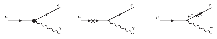
Figure 1: $\mu\rightarrow e\gamma$ with effective anomalous vertices involving the couplings $\alpha$, $\beta$ and $\delta$.

In figure 1 we present the Feynman diagrams for the decay $\mu\rightarrow e\gamma$ (in fact, for any decay of the type $l_{h}\rightarrow l_{l}\gamma$) with vertices containing the effective couplings $\alpha$, $\beta$ and $\delta$. Interestingly, the $\delta$ contributions cancel out, already at the level of the amplitude note2 . The calculation of the remaining diagram is quite simple and gives us the following expression for the width of the anomalous decay $l_{h}\rightarrow l_{l}\gamma$ in terms of the $\alpha$ and $\beta$ couplings:

$$\Gamma(l_{h}\rightarrow l_{l}\gamma) = \frac{m_{h}^{3}}{64\pi\Lambda^{4}}\biggl{[}m_{h}^{2}(|\alpha^{\gamma R}_{lh}+\alpha^{{\gamma R}*}_{hl}|^{2}+|\alpha^{\gamma L}_{lh}+\alpha^{{\gamma L}*}_{hl}|^{2})+16v^{2}(|\beta^{\gamma}_{lh}|^{2}+|\beta^{\gamma}_{hl}|^{2})$$ (15)

$$+ 8m_{h}v\>\mbox{Im}(\alpha^{\gamma R}_{hl}\beta^{\gamma}_{hl}-\alpha^{\gamma R}_{lh}\beta^{\gamma*}_{hl}-\alpha^{\gamma L}_{lh}\beta^{\gamma*}_{lh}+\alpha^{\gamma L}_{hl}\beta^{\gamma}_{lh})\biggr{]}\,\,.$$

So, for the decay $\mu\rightarrow e\gamma$, using the data from pdg , we get (with $\Lambda$ expressed in TeV)

$$\mbox{BR}(\mu\rightarrow e\gamma) = \frac{0.22}{\Lambda^{4}}\biggl{[}(|\alpha^{\gamma R}_{e\mu}+\alpha^{{\gamma R}*}_{\mu e}|^{2}+|\alpha^{\gamma L}_{e\mu}+\alpha^{{\gamma L}*}_{\mu e}|^{2})+4.3\times 10^{7}(|\beta^{\gamma}_{e\mu}|^{2}+|\beta^{\gamma}_{\mu e}|^{2})$$ (16)

$$+ 1.3\times 10^{4}\>\mbox{Im}(\alpha^{\gamma R}_{\mu e}\beta^{\gamma}_{\mu e}-\alpha^{\gamma R}_{e\mu}\beta^{\gamma*}_{\mu e}-\alpha^{\gamma L}_{e\mu}\beta^{\gamma*}_{e\mu}+\alpha^{\gamma L}_{\mu e}\beta^{\gamma}_{e\mu})\biggr{]}\quad\,.$$

Now, all decays $l_{h}\rightarrow l_{l}\gamma$ are severely constrained by experiment pdg especially in the case of $\mu\rightarrow e\gamma$ but also in $\tau\rightarrow e\gamma$ and $\tau\rightarrow\mu\gamma$. To obtain a crude constraint on the couplings, we can use the experimental constraint BR$(\mu\rightarrow e\gamma)<1.2\times 10^{-11}$ and set all couplings but one to zero. With this procedure we get the approximate bound

$$\frac{|\alpha_{e\mu}^{\gamma\,L,R}|}{\Lambda^{2}}\,\leqslant\,7.4\times 10^{-6}\;\;\;\mbox{TeV}^{-2}$$ (17)

and identical bounds for the $\alpha_{\mu e}^{\gamma\,L,R}$ couplings. The constraints on the $\beta$ constants are roughly four orders of magnitude smaller. Using the same procedure for the two remaining LFV processes we get

$$\frac{|\alpha_{e\tau}^{\gamma\,L,R}|}{\Lambda^{2}}\,\leqslant\,1.6\times 10^{-3}\;\;\;\mbox{TeV}^{-2}\qquad\quad\frac{|\alpha_{\mu\tau}^{\gamma\,L,R}|}{\Lambda^{2}}\,\leqslant\,1.3\times 10^{-3}\;\;\;\mbox{TeV}^{-2}$$ (18)

with the $\beta$ couplings even more constrained in their values.

The experimental bounds on the various branching ratios are so stringent that they pretty much curtail any possibility of these anomalous operators having observable effects on any experiences performed at the ILC. To see this, let us consider the flavour-violating reaction $\gamma\,\gamma\,\rightarrow\,l_{h}\,l_{l}$, which in principle could occur at the ILC ggilc . There are five Feynman diagrams involving the $\{\alpha\,,\,\beta\}$ couplings that contribute to this process. There are also three diagrams involving the $\delta$ couplings of eq. (9), but their contributions (once again) cancel at the level of the amplitude. The calculation of the cross section for this process is laborious but unremarkable. The end result, however, is extremely interesting. The cross section is found to be

$$\frac{d\sigma(\gamma\,\gamma\,\rightarrow\,l_{h}\,l_{l})}{dt}\;\;=\;\;-\,\frac{4\pi\alpha\,F_{\gamma\gamma}}{{m_{h}}^{3}\,s\,{({m_{h}}^{2}-t)}^{2}\,t\,{({m_{h}}^{2}-u)}^{2}\,u}\;\Gamma(l_{h}\,\rightarrow\,l_{l}\,\gamma)\;\;\;,$$ (19)

with a function $F_{\gamma\gamma}$ given by

$$F_{\gamma\gamma} =\;\;\;m_{h}^{10}\,(t+u)-12\,m_{h}^{8}\,t\,u+m_{h}^{6}\,(t+u)\,(t^{2}+13\,t\,u+u^{2})-m_{h}^{4}\,t\,u\,(7\,t^{2}+24\,t\,u+7\,u^{2})$$

$$\;\;\;\;\;\;+\,12\,m_{h}^{2}\,t^{2}\,u^{2}\,(t+u)-6\,t^{3}\,u^{3}\;\;\;.$$ (20)

The remarkable thing about eq. (19) is the proportionality of the (differential) cross section to the width of the anomalous decay $l_{h}\,\rightarrow\,l_{l}\,\gamma$, which is to say (modulus the total width of $l_{h}$, which is well known), to its branching ratio. A similar result had been obtained for gluonic flavour-changing vertices in refs. Ferreira:2005dr ; Ferreira:2006xe . Because the allowed branching ratios for the $l_{h}\,\rightarrow\,l_{l}\,\gamma$ are so constrained, the predicted cross sections for the ILC are extremely small. We have

$$\sigma(\gamma\,\gamma\,\rightarrow\,\mu^{-}\,e^{+})\;\sim \;\;\;10^{-8}\,\times\,\mbox{BR}(\mu\,\rightarrow\,e\,\gamma)\;\;\mbox{pb}$$

$$\sigma(\gamma\,\gamma\,\rightarrow\,\tau^{-}\,\mu^{+})\;\sim \;\;\;10^{-5}\,\times\,\mbox{BR}(\tau\,\rightarrow\,\mu\,\gamma)\;\;\mbox{pb}$$

$$\sigma(\gamma\,\gamma\,\rightarrow\,\tau^{-}\,e^{+})\;\sim \;\;\;10^{-5}\,\times\,\mbox{BR}(\tau\,\rightarrow\,e\,\gamma)\;\;\mbox{pb}\;\;\;,$$ (21)

with $\sqrt{s}\,=\,1$ TeV. With the current branching ratios of the order of $10^{-12}$ for the muon decay and $10^{-7}$ for the tau ones, it becomes obvious that these reactions would have unobservable cross sections.

Our conclusion is thus that the $\alpha_{ij}^{\gamma}$ and $\beta_{ij}^{\gamma}$ couplings are too small to produce observable signals in foreseeable collider experiments. However, both $\{\alpha^{\gamma}_{ij}\,,\,\beta^{\gamma}_{ij}\}$ and $\{\alpha^{Z}_{ij}\,,\,\beta^{Z}_{ij}\}$ are written in terms of the original $\{\alpha^{B,W}_{ij}\,,\,\beta^{B,W}_{ij}\}$ couplings, via coefficients (sine and cosine of $\theta_{W}$) of order 1. Hence, unless there was some bizarre unnatural cancellation, the couplings $\{\gamma\,,\,Z\}$ and $\{B\,,\,W\}$ should be of the same order of magnitude. Since we have no reason to assume such a cancellation, we come to the conclusion that the $\alpha$ and $\beta$ couplings are simply too small to be considered interesting. They will have no bearing whatsoever on anomalous LFV interactions mediated by the $Z$ boson. From now on, we will simply consider them to be zero, which means that there will not be any anomalous vertices of the form $\gamma\,l_{i}\,l_{j}$.

III.2 A set of free parameters

In the previous section we have presented the complete set of operators that give contributions to the flavour violating processes $e^{+}e^{-}\rightarrow l_{h}l_{l}$. However, these operators are not, a priori, all independent. It can be shown that (see refs. buch ; Ferreira:2005dr ; Grzadkowski:2003tf ; Ferr3 for details), for instance, there is a relation between operators of the types ${\cal O}_{eB\phi}$ and ${\cal O}_{eB}$ and some of the four fermion operators, modulo a total derivative. These relations between operators appear when one uses the fermionic equations of motion, along with integration by parts. They could be used to discard operators whose coupling constants are $\alpha$ and $\beta$, or some of the four fermion operators. We used this argument to present the results in refs. Ferreira:2005dr ; Ferreira:2006xe ; Ferr3 in a more simplified fashion. However, in the present circumstances, we already discarded the $\alpha$ and $\beta$ operators due to the size of their contributions to physical processes being extremely limited by the existing bounds on flavour-violating leptonic decays with a photon. Since we already threw away these two sets of operators, we are not entitled to use the equations of motion to attempt to eliminate another.
Notice also that in most of the work that was done with the effective lagrangian approach one replaces, at the level of the amplitude, operators of the type ${\cal O}_{D_{e}}$ by operators of the type ${\cal O}_{eZ\phi}$ by using Gordon identities. In fact, it can be shown that the following relation holds for free fermionic fields,

$$\bar{e}^{i}_{L}\,\partial^{\mu}\,e^{j}_{R}\,=\,m_{j}\,\bar{e}^{i}_{L}\,\gamma^{\mu}\,e^{j}_{R}-\bar{e}^{i}_{L}\,\sigma^{\mu\alpha}\ \partial^{\alpha}\,e^{j}_{R}\,\,.$$ (22)

Notice that the use of Gordon identities is not the same thing as using the field’s equations of motion to eliminate operators: in the latter case, one proves that different operators are related to one another and use those conditions to choose among them; in the former, all we are doing is re-writing the amplitude in a different form. And in our case, this procedure does not bring any simplification.
Finally, using the equations of motion, a relation can be established between operators ${\cal O}_{D_{e}}$ and ${\cal O}_{\bar{D}_{e}}$, namely

$${\cal O}_{D_{e}}+{\cal O}_{\bar{D}_{e}}+\left(\bar{\ell}_{L}\,e_{R}\right)\,\left[\Gamma_{e}^{\dagger}\bar{e}_{R}\,\ell_{L}+\Gamma_{u}\bar{q}_{L}\epsilon\,u_{R}+\Gamma_{d}^{\dagger}\bar{d}_{R}\,q_{L}\right]\,=\,0\;\;\;,$$ (23)

where the $\Gamma_{e}$ coefficients are the leptonic Yukawa couplings and $\epsilon$ the bidimensional Levi-Civita tensor. We see that the relationship between these two operators involves four-fermion terms as well. This relation means we can choose between one of the two operators ${\cal O}_{D_{e}}$ and ${\cal O}_{\bar{D}_{e}}$, given that the four-fermion operators appearing in this expression have already been considered by us. This means that only one of the $\eta_{ij}^{R}$ and $\eta_{ij}^{L}$ couplings will appear in the calculation. We chose the first one and will drop, from this point onwards, the superscript “$R$”. Also, after expanding the operators of eq. (3), we see that the $\theta$ couplings always appear in the same combinations. We therefore define two new couplings, $\theta_{R}$ and $\theta_{L}$, as

$$\theta_{R}\;=\;\theta_{lh}^{R}+\theta_{hl}^{R*}\;\;\;,\;\;\;\theta_{L}\;=\;\theta_{lh}^{L(1)}+\theta_{hl}^{L(1)*}-\theta_{lh}^{L(3)}-\theta_{hl}^{L(3)*}\;\;\;.$$ (24)

As an aside, we must add that the use of equations of motion to simplify the effective lagrangian is not followed by all authors. For instance, the authors of whi do not use them and consider instead a fully general set of dimension six effective operators.
The original lagrangian is now reduced to

$${\cal L}\;\;=\;\;\;{\cal L}_{eel_{l}l_{h}}\;+\;{\cal O}_{D_{e}}\;+\;{\cal O}_{\phi e}\;+\;{\cal O}^{(1)}_{\phi\ell}\;+\;{\cal O}^{(3)}_{\phi\ell}\;+\;{\cal O}_{e\ell\phi}\;+\;\mbox{h.c.}\qquad.$$ (25)

We will not present the Feynman rules for the four fermion interactions because they are obvious and rather cumbersome to write. The remaining Feynman rules we will use are presented in figure 2, where lepton momenta follow the arrows and vector boson momentum is incoming. For completeness, we included the

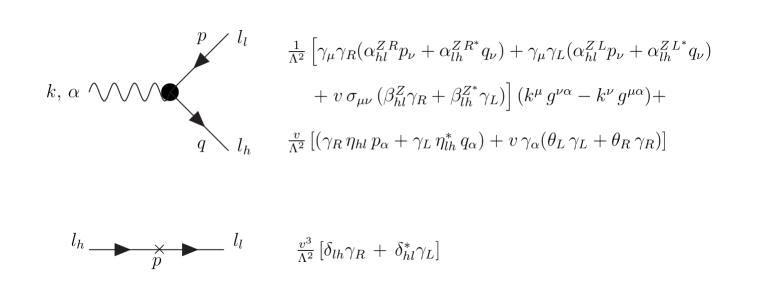
Figure 2: Feynman rules for anomalous $Z\,\bar{l_{h}}\,l_{l}$ and $\bar{l_{l}}\,l_{h}$ vertices.

$\alpha^{Z}_{ij}$ and $\beta^{Z}_{ij}$ in this figure, but we remind the reader that we have set them to zero.

IV Decay widths

As we said before, all LFV processes are severely constrained by experimental data. Now that we have settled on a set of anomalous effective operators, we should first consider what is the effect of those operators on LFV decays. The existing data severely constrains two types of decay: a heavy lepton decaying into three light ones, $l_{h}\,\rightarrow\,l\,l\,l$, such as $\tau^{-}\,\rightarrow\,e^{-}\,e^{+}\,e^{-}$, and decays of the Z boson to two different leptons, $Z\,\rightarrow\,l_{h}\,l_{l}$ (such as $Z\,\rightarrow\,\tau^{+}\,e^{-}$). Flavour-violating processes involving neutrinos in the final state (such as, say, $Z\,\rightarrow\,\nu_{\tau}\,\bar{\nu}_{e}$) are not constrained by experimental data, as they are indistinguishable from the “normal” processes.

For the 3-lepton decay, there are three distinct contributions, whose Feynman diagrams are shown in figure 3 for the particular case of $\mu^{-}\,\rightarrow\,e^{-}\,e^{+}\,e^{-}$. As before, the contributions involving the $\delta$ operators cancel at the level of the amplitude and have absolutely no effect on the physics. Using the Feynman rules in figure 2 and the four fermion lagrangian we can determine the expression for the decay $l_{h}\rightarrow lll$. Remember that $l$ stands for a massless lepton whatever its flavour is.

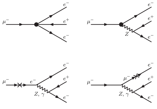
Figure 3: Feynman diagrams for the decay $\mu^{-}\,\rightarrow\,e^{-}\,e^{+}\,e^{-}$.

The decay width obtained is the sum of three terms, to wit

$$\Gamma(l_{h}\,\rightarrow\,l\,l\,l)\;=\;\Gamma_{4f}(l_{h}\,\rightarrow\,l\,l\,l)\,+\,\Gamma_{Z}(l_{h}\,\rightarrow\,l\,l\,l)\,+\,\Gamma_{int}(l_{h}\,\rightarrow\,l\,l\,l)\;\;\;,$$ (26)

where $\Gamma_{4f}$ contains the contributions from the four-fermion graph in figure 3, $\Gamma_{Z}$ those from the Feynman diagram with a Z boson and $\Gamma_{int}$ the interference between both diagrams. A simple calculation yields

$$\Gamma_{4f}(l_{h}\,\rightarrow\,l\,l\,l)\;= \frac{m_{h}^{5}}{6144\,\pi^{3}\,\Lambda^{4}}\,\left[|S_{LR}|^{2}+|S_{RL}|^{2}+4(|V_{LL}|^{2}+|V_{RR}|^{2})\right]\vspace{0.3cm}$$

$$\Gamma_{Z}(l_{h}\,\rightarrow\,l\,l\,l)\;= \;\;\frac{(g_{A}^{2}+g_{V}^{2})v^{2}}{768\,M_{z}^{4}\,\pi^{3}\,\Lambda^{4}}\,\left\{\left(|\theta_{L}|^{2}+|\theta_{R}|^{2}\right)v^{2}m_{h}^{5}+\frac{1}{2}\mbox{Re}\left(\eta_{lh}\theta_{L}^{*}+\eta_{hl}\theta_{R}^{*}\right)v\,m_{h}^{6}\right.\vspace{0.3cm}$$

$$\;\;\left.+\frac{m_{h}^{7}}{10M_{z}^{2}}\left[(|\eta_{lh}|^{2}+|\eta_{hl}|^{2})M_{z}^{2}+6(|\theta_{L}|^{2}+|\theta_{R}|^{2})\,v^{2}\right]\right\}$$

$$\Gamma_{int}(l_{h}\,\rightarrow\,l\,l\,l)\;= \;\;\frac{v^{2}\,m_{h}^{5}}{768M_{z}^{2}\pi^{3}\Lambda^{4}}\,\left[\left(1+\frac{3m_{h}^{2}}{10M_{z}^{2}}\right)\biggl{\{}\left(g_{V}+g_{A}\right)\mbox{Re}\left(\theta_{L}V_{LL}^{*}\right)+\right.\vspace{0.3cm}$$

$$\;\left(g_{V}-g_{A}\right)\mbox{Re}\left(\theta_{R}V_{RR}^{*}\right)\biggr{\}}-\frac{m_{h}}{4v}\left(1+\frac{m_{h}^{2}}{5M_{z}^{2}}\right)\biggl{\{}\left(g_{V}+g_{A}\right)\mbox{Re}\left(\eta_{lh}V_{RR}^{*}\right)+\vspace{0.3cm}$$

$$\;\left(g_{V}-g_{A}\right)\mbox{Re}\left(\eta_{hl}V_{LL}\right)\biggr{\}}\biggr{]}\;\;\;.$$ (27)

where

$$g_{V}\;=\;-\,\frac{e}{\sin\theta_{W}\,\cos\theta_{W}}\left(-\frac{1}{4}+\sin\theta_{W}^{2}\right)\;\;\;,\;\;\;g_{A}\;=\;\,\frac{e}{4\sin\theta_{W}\,\cos\theta_{W}}$$ (28)

and $e$ is the elementary electric charge. An important remark about these results: they are not, in fact, the exact expressions for the decay widths. The full expressions for $\Gamma_{Z}(l_{h}\,\rightarrow\,l\,l\,l)$ and $\Gamma_{int}(l_{h}\,\rightarrow\,l\,l\,l)$ are actually the sum of a logarithmic term and a polynomial one. However, it so happens that the first four terms of the Taylor expansion in $m_{h}/M_{z}$ of the logarithm cancel the polynomial exactly. The expressions of eq. (27) are therefore the first surviving terms of that Taylor expansion, and constitute an excellent approximation to the exact result, and one that is much easier to deal with numerically (the cancellation mentioned poses a real problem in numerical calculations).

As for the LFV decays of the Z-boson, there is an extensive literature on this subject zes . There are, of course, no four fermion contributions to this decay width, and a simple calculation provides us the following expression:

$$\Gamma(Z\,\rightarrow\,l_{h}\,l_{l})\;= \;\;\frac{(M_{z}^{2}-m_{h}^{2})^{2}\,v^{2}}{128\,M_{z}^{5}\,\pi\,\Lambda^{4}}\,\left[(M_{z}^{2}-m_{h}^{2})^{2}(|\eta_{hl}|^{2}+|\eta_{lh}|^{2})+4\,(m_{h}^{2}+2M_{z}^{2})v^{2}(|\theta_{L}|^{2}+|\theta_{R}|^{2})\right.\vspace{0.3cm}$$

$$\;\left.\;+\,4\,m_{h}\,(m_{h}^{2}-M_{z}^{2})\,v\,\mbox{Re}\left(\theta_{L}\eta_{hl}+\theta_{R}\eta_{lh}^{*}\right)\right]\;\;\;.$$ (29)

V Cross Sections

In this section we will present expressions for the cross sections of various LFV processes that may occur at the ILC. There are three such processes, namely (1) $e^{+}e^{-}\rightarrow\mu^{-}e^{+}$, (2) $e^{+}e^{-}\rightarrow\tau^{-}e^{+}$ and (3) $e^{+}e^{-}\rightarrow\tau^{-}\mu^{+}$, as well as the respective charge-conjugates. We have calculated all cross sections keeping both final state masses. However, given the energies involved, the contributions to the cross sections which arise from the lepton masses are extremely small, and setting them to zero is an excellent approximation. We thus present all formulae with zero leptonic masses, as they are much simpler than the complete expressions. In figures 4 and 5 we present all diagrams that contribute to the process $e^{+}e^{-}\rightarrow\mu^{-}e^{+}$.

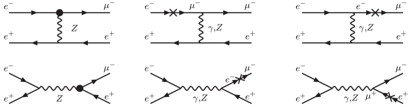
Figure 4: Feynman diagrams describing the process $e^{+}e^{-}\rightarrow\mu^{-}e^{+}$

A brief word about our conventions. There are two types of LFV production cross sections, corresponding to different sets of Feynman diagrams. In the case of process (1), we see from figures 4 and 5 that the reaction

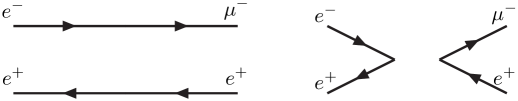
Figure 5: Interpretation of the four fermion terms contributing to the process $e^{+}e^{-}\rightarrow\mu^{-}e^{+}$ in terms of currents; notice the analog of a $t$ channel and an $s$ one.

can proceed through both a $t$-channel and an $s$-channel - this is obvious for the diagrams involving the exchange of a photon or a $Z$ boson. For the four-fermion channels less so, but figure 5 illustrates the $t$ and $s$-channel analogy. Depending on the “location” of the incoming electron spinor in the operators of eq. (5), we can interpret those operators as two fermionic currents interacting with one another, that interaction is obviously analog to the two different channels. Process (2) has diagrams identical to those of process (1). Process (3), however, can only occur through the $s$ channel - that is obvious once one realizes that for process (3) there is no positron in the final state. In fact for process (3) there are only “s-channel” contributions from the four-fermion operators.

A simple way of condensing the different four-fermion cross sections into a single expression is to adopt the following convention: we will include indices “s” and “t” in the four fermion couplings. If we are interested in the cross sections for processes (1) and (2) - which occur through both $s$ and $t$ channels - then all “s” couplings will be equal to the “t” ones. If we wish to obtain the cross section for process (3) (which only has $s$ channels) we must simply set all couplings with a “t” index to zero. We have further considered the likely possibility that in the ILC one may be able to polarize the beams of incoming electrons and positrons Moortgat-Pick:2005cw . Thus, $\sigma_{IJ}$ represents the polarized cross section for an $I$ polarized electron and a $J$ polarized positron, with $\{I\,,\,J\}\,=\,\{R\,,\,L\}$ - that is, beams with a right-handed polarization or a left-handed one. The explicit expressions for the four-fermion differential cross sections are then given by

$$\frac{d\sigma_{LL}}{dt}\,= \,\frac{1}{16\pi s^{2}\Lambda^{4}}\left[4u^{2}|V_{LL}^{s}+V_{LL}^{t}|^{2}+t^{2}(4|V_{LR}^{s}|^{2}+|S_{RL}^{t}|^{2})\right]$$

$$\frac{d\sigma_{RR}}{dt}\,= \,\frac{1}{16\pi s^{2}\Lambda^{4}}\left[4u^{2}|V_{RR}^{s}+V_{RR}^{t}|^{2}+t^{2}(4|V_{RL}^{s}|^{2}+|S_{LR}^{t}|^{2})\right]$$

$$\frac{d\sigma_{LR}}{dt}\,= \,\frac{1}{16\pi s^{2}\Lambda^{4}}\left[u^{2}|S_{LL}^{s}+S_{LL}^{t}|^{2}+s^{2}(4|V_{RL}^{t}|^{2}+|S_{LR}^{s}|^{2})\right]$$

$$\frac{d\sigma_{RL}}{dt}\,= \,\frac{1}{16\pi s^{2}\Lambda^{4}}\left[u^{2}|S_{RR}^{s}+S_{RR}^{t}|^{2}+s^{2}(4|V_{LR}^{t}|^{2}+|S_{RL}^{s}|^{2})\right]$$ (30)

See appendix B for the full calculation. The unpolarized cross section is obviously the averaged sum over the four terms of eq. (30). To re-emphasize, the four-fermion cross section for processes (1) and (2) is obtained from this expression by setting all “s” couplings equal to the “t” ones; and to obtain the cross section for process (3) one must simply set all “t” couplings to zero.
The total cross sections for each of the processes are then given by

$$\sigma^{(1,2)}(e^{-}e^{+}\rightarrow l_{h}e^{+}) =\;\;\sigma_{Z}^{(1,2)}\,+\,\sigma_{4f}^{(1,2)}\,+\,\sigma_{int}^{(1,2)}$$

$$\sigma^{(3)}(e^{-}e^{+}\rightarrow\tau^{-}\mu^{+}) =\;\;\sigma_{Z}^{(3)}\,+\,\sigma_{4f}^{(3)}\,+\,\sigma_{int}^{(3)}\;\;\;,$$ (31)

where $\sigma_{Z}$ is the cross section involving only the anomalous $Z$ interactions of figure 2, $\sigma_{4f}$ the four-fermion cross section - whose calculation we already explained - and $\sigma_{int}$ the interference between both of these. The $\delta$ couplings also present in figure 2 end up not contributing at all to the physical cross sections, once again. For completeness, then, the remaining terms in the differential cross section for processes (1) and (2) are given by

$$\frac{d\sigma_{Z}^{(1,2)}}{dt}\;=-v^{2}\,\frac{v^{2}\,\left[F_{1}(g_{A},g_{V})\,|\theta_{L}|^{2}+F_{1}(g_{A},-g_{V})|\theta_{R}|^{2}\right]\,+\,F_{2}(g_{A},g_{V})\,|\eta_{lh}|^{2}+F_{2}(g_{A},-g_{V})|\eta_{hl}|^{2}}{32\,\pi\,\Lambda^{4}\,{\left(M_{z}^{2}-s\right)}^{2}\,s^{2}\,{\left(M_{z}^{2}-t\right)}^{2}}$$ (32)

with

$$F_{1}(g_{A},g_{V})\,= \,2\,\left\{(g_{A}+g_{V})^{2}\left[s\,t\,(2\,M_{z}^{4}+2\,u\,M_{z}^{2}+s^{2}+t^{2})-u\,M_{z}^{2}\,(u\,M_{z}^{2}+2\,s^{2}+2\,t^{2})\right]\right.+$$

$$\left.2\,(g_{A}^{2}+g_{V}^{2})u\,(t^{3}+s^{3})+(g_{A}-g_{V})^{2}s\,u^{2}\,t\right\}$$

$$F_{2}(g_{A},g_{V})\,= \,-t\,u\,s\,\left[(g_{A}^{2}+g_{V}^{2})(3\,M_{z}^{4}+3\,u\,M_{z}^{2}+s^{2}+t^{2}+s\,t)+2\,g_{A}\,g_{V}\,\left(M_{z}^{2}-s\right)\,\left(M_{z}^{2}-t\right)\right]\;\;\;.$$ (33)

The interference term is given by

$$\frac{d\sigma_{int}^{(1,2)}}{dt}\;= \,\frac{(t-s)\,v^{2}}{16\,\pi\,\Lambda^{4}\,\left(M_{z}^{2}-s\right)\,s^{2}\,\left(M_{z}^{2}-t\right)}$$

$$\biggl{[}\left(g_{A}\,\mbox{Re}\left(\theta_{L}S_{LR}^{*}-\theta_{R}S_{RL}^{*}\right)+g_{V}\,\mbox{Re}\left(\theta_{L}S_{LR}^{*}+\theta_{R}S_{RL}^{*}\right)\right)\,\left(s\,t+\left(-M_{z}^{2}+s+t\right)\,u\right)$$

$$+\,4\,(g_{A}-g_{V})\,(s+t)\,u\,\mbox{Re}\left(\theta_{L}V_{LL}^{*}\right)-4\,(g_{A}+g_{V})\,(s+t)\,u\,\mbox{Re}\left(\theta_{R}V_{RR}^{*}\right)\biggr{]}$$ (34)

For process (3), we have

$$\frac{d\sigma_{Z}^{(3)}}{dt}\,= \,\frac{-v^{2}}{32\,\pi\,\Lambda^{4}\,{\left(M_{z}^{2}-s\right)}^{2}\,s^{2}}\biggl{\{}2\,v^{2}\left[(g_{A}^{2}+g_{V}^{2})\,(2tu-s^{2})\,(|\theta_{L}|^{2}+|\theta_{R}|^{2})\right.$$

$$\left.+\,2\,g_{A}\,g_{V}\,s(t-u)\,(|\theta_{L}|^{2}-|\theta_{R}|^{2})\right]-(g_{A}^{2}+g_{V}^{2})\,t\,u\,s\,(|\eta_{hl}|^{2}+|\eta_{lh}|^{2})\biggr{\}}$$ (35)

and finally, the interference terms are

$$\frac{d\sigma_{int}^{(3)}}{dt}=\frac{(s+t)\,u\,v^{2}}{8\,\pi\,\Lambda^{4}\,\left(M_{z}^{2}-s\right)\,s^{2}}\biggl{[}(g_{V}-g_{A})\,Re\left(\theta_{L}V_{LL}^{*}\right)+(g_{V}+g_{A})\,\mbox{Re}\left(\theta_{R}V_{RR}^{*}\right)\biggr{]}\;\;\;.$$ (36)

At this point we must remark on the different energy behavior that these various terms follow. Once integrated in $t$, the four-fermion terms grow linearly with $s$, whereas those arising from the anomalous $Z$ couplings have a much smoother evolution with $s$ - whereas the first ones diverge as $s\,\rightarrow\,\infty$, the second ones tend to zero. See appendix B for the expressions of the integrated cross sections. This could be interpreted as a clear dominance of the four-fermion terms over the remaining anomalous couplings. However, we must remember that we are working in a non-renormalizable formalism. We know, from the beginning, that these operators only offer a reasonable description of high-energy physics up to a given scale, of the order of $\Lambda$. The dominance of the four-fermion cross section must therefore be carefully considered - it may simply happen, as there is nothing preventing it, that the four-fermion couplings of eq. (5) are much smaller in size than the $Z$ boson ones of figure 2.

As we saw, the $\delta$ couplings end up not contributing to either decay widths or cross sections (and this is true regardless of whether the light leptons are considered massless or not). As we mentioned before, their inclusion could be interpreted as an on-shell renormalization of the leptonic propagators. On that light, their cancellation suggests that the effective operator formalism is equivalent to an on-shell renormalization scheme. This is further supported by the fact that the list of effective operators of ref. buch was obtained by using the fields’ equations of motion to simplify several terms. However, we must mention that at least in some Feynman diagrams (some of those contributing to $\gamma\,\gamma\,\rightarrow\,l_{h}\,l_{l}$, for instance), the “$\delta$-insertions” were made in internal fermionic lines, so that this cancellation is not altogether obvious.

V.1 Asymmetries

In a collider with polarized beams, asymmetries can play a major role in the determination of flavour-violating couplings. A great advantage of using these observables is that, as will soon become obvious, all dependence on the scale of unknown physics, $\Lambda$, vanishes due to their definition. There is a strong possibility that the ILC could have both beams polarized, therefore the measurement of polarization asymmetries could be very interesting. For a more detailed study see Moortgat-Pick:2005cw . A particulary appealing situation is found when the contributions from the $Z$ boson anomalous couplings are not significant when compared with the four fermion ones. In this case the study of asymmetries would allow us, in principle, to determine each four-fermion coupling individually. We will now concentrate on one of the most feasible scenarios, which is to have a polarized electron beam and an unpolarized positron beam. We will take both the right-handed and left-handed polarizations to be 100%, which is obviously above what is expected to occur (recent studies show that a 90 % polarization is attainable) Moortgat-Pick:2005cw . The differential cross sections for left-handed ($P_{e^{-}}=-1$) and right-handed ($P_{e^{-}}=+1$) polarized electrons are

$$\frac{d\sigma_{L}}{dt}\,= \,\frac{1}{16\pi s^{2}\Lambda^{4}}\left(4u^{2}|V_{LL}^{s}+V_{LL}^{t}|^{2}+t^{2}|S_{RL}^{t}|^{2}+s^{2}|S_{LR}^{s}|^{2}\right)$$

$$\frac{d\sigma_{R}}{dt}\,= \,\frac{1}{16\pi s^{2}\Lambda^{4}}\left(4u^{2}|V_{RR}^{s}+V_{RR}^{t}|^{2}+t^{2}|S_{LR}^{t}|^{2}+s^{2}|S_{RL}^{s}|^{2}\right)\,\,.$$ (37)

Two forward-backward asymmetries for the left-handed and right-handed polarized cross sections can now be defined as

$$A_{FB,L(R)}\,=\,\frac{\int_{0}^{\pi/2}d\sigma_{L(R)}(\theta)\,-\,\int_{\pi/2}^{\pi}d\sigma_{L(R)}(\theta)}{\sigma_{L(R)}}$$ (38)

and we can also define a left-right asymmetry, given by

$$A_{LR}\,=\,\frac{\sigma_{L}-\sigma_{R}}{\sigma_{L}+\sigma_{R}}\;\;\;,$$ (39)

where $\sigma_{L(R)}$ is the total cross section for a left-handed (right-handed) polarized electron beam. Note that we have assumed that the polarization of the final state particles is not measured. Otherwise we could get even more information by building an asymmetry related to the measured final state polarizations. Using the expressions on appendix B it is simple to find, for these asymmetries, the following expressions:

$$A_{FB,L}\,=\,\frac{12\,|V_{LL}^{s}+V_{LL}^{t}|^{2}-3\,|S_{RL}^{t}|^{2}}{16\,|V_{LL}^{s}+V_{LL}^{t}|^{2}+4\,|S_{RL}^{t}|^{2}+12\,|S_{LR}^{s}|^{2}}$$ (40)

and

$$A_{FB,R}\,=\,\frac{12\,|V_{RR}^{s}+V_{RR}^{t}|^{2}-3\,|S_{LR}^{t}|^{2}}{16\,|V_{RR}^{s}+V_{RR}^{t}|^{2}+4\,|S_{LR}^{t}|^{2}+12\,|S_{RL}^{s}|^{2}}\,\,.$$ (41)

Finally, the left-right asymmetry reads

$$A_{LR}\,=\,\frac{|V_{LL}^{s}+V_{LL}^{t}|^{2}-|V_{RR}^{s}+V_{RR}^{t}|^{2}+|S_{RL}^{t}|^{2}-|S_{LR}^{t}|^{2}+3\,(|S_{LR}^{s}|^{2}-|S_{RL}^{s}|^{2})}{|V_{LL}^{s}+V_{LL}^{t}|^{2}+|V_{RR}^{s}+V_{RR}^{t}|^{2}+|S_{RL}^{t}|^{2}+|S_{LR}^{t}|^{2}+3\,(|S_{LR}^{s}|^{2}+|S_{RL}^{s}|^{2})}\,,$$ (42)

which has no dependence on $\Lambda$. Notice that all of these expressions assume an unpolarized positron beam, and a completely polarized electron beam, either left- or right-handed. If the electron beam is not perfectly polarized, but instead has a percentage of polarization $P_{e^{-}}$, we can still write

$$\sigma_{P_{e^{-}}}\,=\,\sigma_{0}\left[1-P_{e^{-}}A_{LR}\right]$$ (43)

with $\sigma_{0}\,=\,(\sigma_{L}+\sigma_{R})/4$. So if in reality we only have access at the ILC to beams with +80 % (- 80 %) polarization we could still use them to determine $\sigma_{0}$ and $A_{LR}$. If we had access to a positron polarized beam, we could then write a similar expression for the cross section obtained from the polarized positrons. Notice that $A_{LR}$ would be different - the indices left and right would then refer to the positron and not to the electron.

The most interesting possibility is, of course, when both beams are polarized, with different percentages, $P_{e^{-}}$ and $P_{e^{+}}$. We could then perform experiments where the four different combinations of beam polarizations were used. The resulting cross section would be

$$\sigma_{P_{e^{-}}P_{e^{+}}}\,= \,\frac{1}{4}\biggl{[}(1+P_{e^{-}})(1+P_{e^{+}})\sigma_{RR}\,+\,(1-P_{e^{-}})(1-P_{e^{+}})\sigma_{LL}+$$

$$(1+P_{e^{-}})(1-P_{e^{+}})\sigma_{RL}\,+\,(1-P_{e^{-}})(1+P_{e^{+}})\sigma_{LR}\biggr{]}\;\;\;.$$ (44)

As such, we would be able to determine $\sigma_{RR}$, $\sigma_{LL}$, $\sigma_{RL}$ and $\sigma_{LR}$ - and consequently each of the four four-fermion couplings, $V_{LL}$, $V_{RR}$, $S_{RL}$ and $S_{LR}$.

VI Results and Discussion

In the previous sections we computed cross sections and decay widths for several flavour-violating processes. We will now consider the possibility of their observation at the ILC. To do so we will use one set of parameters Moortgat-Pick:2005cw for the ILC, i.e., a center-of mass energy of $\sqrt{s}=1$ TeV and an integrated luminosity of ${\cal L}=1$ ab^-1. At this point we remark that, other than the experimental constraints on the flavour-violating decay widths computed in sec. IV (see table 1), we have no bounds on the values of the anomalous couplings. The range of values chosen for each of the coupling constants was $10^{-4}\leq|a/\Lambda^{2}|\leq 10^{-1}$, where $a$ stands for a generic coupling and $\Lambda$ is in TeV. For $a\approx 1$ the scale of new physics can be as large as 100 TeV. This means that if the scale for LFV is much larger than 100 TeV, it will not be probed at the ILC unless the values of coupling constants are unusually large. The asymmetry plots are not affected by this choice as explained before.

Table 1: Experimental constraints on flavour-violating decay branching ratios pdg .

Process	Upper bound
$\tau\,\rightarrow\,e\,e\,e$	$2.0\times 10^{-7}$
$\tau\,\rightarrow\,e\,\mu\,\mu$	$2.0\times 10^{-7}$
$\tau\,\rightarrow\,\mu\,e\,e$	$1.1\times 10^{-7}$
$\tau\,\rightarrow\,\mu\,\mu\,\mu$	$1.9\times 10^{-7}$
$\mu\,\rightarrow\,e\,e\,e$	$1.0\times 10^{-12}$
$Z\,\rightarrow\,e\,\mu$	$1.7\times 10^{-6}$
$Z\,\rightarrow\,e\,\tau$	$9.8\times 10^{-6}$
$Z\,\rightarrow\,\tau\,\mu$	$1.2\times 10^{-5}$

We will therefore generate random values for all anomalous couplings (four-fermion and $Z$ alike), and discard those combinations of values of the couplings for which the several branching ratios we computed earlier are larger than the corresponding experimental upper bounds from table 1. This procedure allows for the possibility that one set of anomalous couplings (the $Z$ or four-fermion ones) might be much larger than the other. When an acceptable combination of values is found, it is used in expressions (30)- (36) to compute the value of the flavour-violating cross section. In figure 6 we plot the number of events expected at the ILC for the process

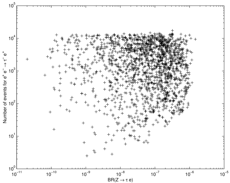
Figure 6: Number of expected events at the ILC for the reaction $e^{+}\,e^{-}\,\rightarrow\,\tau^{-}\,e^{+}$, with a center-of-mass energy of 1 TeV and a total luminosity of 1 ab^-1.

$e^{+}\,e^{-}\,\rightarrow\,\tau^{-}\,e^{+}$, in terms of the branching ratio BR$(Z\,\rightarrow\,\tau\,e)$. To obtain the points shown in this graph, we demanded that the values of the effective couplings were such that all of the branching ratios for the decays of the $\tau$ lepton into three light leptons and BR$(Z\,\rightarrow\,\tau\,\mu)$ were smaller than the experimental upper bounds on those quantities shown in table 1. We observe that, even for fairly small values of the $\tau$ flavour-violating decay branching ratios ($10^{-9}$-$10^{-6}$), there is the possibility of a large number of events for the anomalous cross section.

By following the opposite procedure - requiring first that the branching ratios BR$(Z\,\rightarrow\,\tau\,e)$ and BR$(Z\,\rightarrow\,\tau\,\mu)$ be according to the experimental values, and letting BR$(\tau\,\rightarrow\,l\,l\,l)$ free, where $l$ is either an electron or a muon - we obtain the plot shown in figure 7. This time we analyse the process

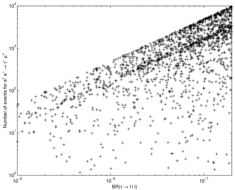
Figure 7: Number of expected events at the ILC for the reaction $e^{+}\,e^{-}\,\rightarrow\,\tau^{-}\,\mu^{+}$, with a center-of-mass energy of 1 TeV and a total luminosity of 1 ab^-1.

$e^{+}\,e^{-}\,\rightarrow\,\tau^{-}\,\mu^{+}$, but a similar plot is found for $e^{+}\,e^{-}\,\rightarrow\,\tau^{-}\,e^{+}$. The number of events rises sharply with increasing branching ratio of $\tau$ into three leptons. It is possible to discern a thin “band” of events in the middle of the points of figure 7, rising linearly with BR$(\tau\,\rightarrow\,l\,l\,l)$. This “band” corresponds to events for which the four-fermion couplings are dominant over $Z^{0}$ events. In that case, they dominate both BR$(\tau\,\rightarrow\,l\,l\,l)$ and $\sigma(e^{+}\,e^{-}\,\rightarrow\,\tau^{-}\,\mu^{+})$, and the larger one is, the larger the other will be - which explains the linear growth of this subset of points in the plot of figure 7. This “isolated” contribution from the four-fermion terms is not visible in figure 6 since the branching ratios of the $Z$ decays are independent of those same couplings. Finally and for completeness, in figure 8 we show the values of the asymmetry

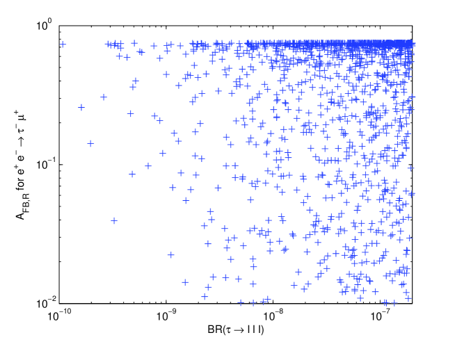
Figure 8: $A_{FB,R}$ asymmetry for the process $e^{+}\,e^{-}\,\rightarrow\,\tau^{-}\,\mu^{+}$ versus $BR(\tau\,\rightarrow\,l\,l\,l)$

coefficient $A_{FB,R}$ defined in (41), for the process $e^{+}\,e^{-}\,\rightarrow\,\tau^{-}\,\mu^{+}$, versus the three-lepton decay of the $\tau$. A similar plot is obtained for the asymmetry $A_{FB,L}$. We observe a fairly uniform dependence on the branching ratio $BR(\tau\,\rightarrow\,l\,l\,l)$, which is to say, on the values of the four-fermion couplings. However, there is a significant concentration of “points” near the maximum allowed value for this cross section, 0.75.

Finally, we also considered another possible process of LFV, namely $\gamma\,e^{-}\,\rightarrow\,\mu^{-}\,Z^{0}$. There are three Feynman diagrams contributing to this process, one of which involving a quartic vertex which emerges from the effective operators of eqs. (2) and (3). This process might occur at the ILC, if we consider the almost-collinear photons emitted by the colliding leptons, well described by the so-called equivalent photon approximation (EPA) epa . An estimate of the cross section for this process, however, showed it to be much lower than the remaining ones we considered in this paper. This is due to the EPA introducing an extra electromagnetic coupling constant into the cross section, and also to the fact that the final state of this process includes at least three particles (one of the beam particles “survives” the interaction)- thus there is, compared to the other processes which have only leptons in the final state, an additional phase space suppression. Notice, however, that an optional upgrade for the ILC is to have $e\,\gamma$ collisions, with center-of-mass energies and luminosities similar to those of the $e^{+}\,e^{-}$ mode, so this cross section might become important.

The flavour-violating channels are experimentally interesting, as they present a final state with an extremely clear signal, which can be easily identified. The argument is that the final state will always present two very energetic leptons of different flavour, more to the point, an electron and a muon. LFV can be seen in one of the three channels $e^{+}e^{-}\rightarrow\mu^{-}e^{+}$, $e^{+}e^{-}\rightarrow\tau^{-}e^{+}$, $e^{+}e^{-}\rightarrow\tau^{-}\mu^{+}$ and charge conjugate channels. The first channel is the best one, with the two leptons back to back and almost free of backgrounds. For the other production processes, we may “select” the decays of the tau that best suit our purposes: for the second we should take the tau decay $\tau^{-}\rightarrow\mu^{-}\bar{\nu_{\mu}}\nu_{\tau}$, and for the third process, $\tau^{-}\rightarrow e^{-}\bar{\nu_{e}}\nu_{\tau}$. The branching ratios for both of these tau decays are around 17%, so the loss of signal is affordable. The conclusion is that, for every lepton flavour-violating process, one can always end up with a final state with an electron and a muon. If the ILC detectors have superb detection performances for these particles, then the odds of observing violation of the leptonic number at the ILC, if those processes do exist, seem reasonable.

Clearly, our prediction that significant numbers of anomalous events may be produced at the ILC needs to be further investigated including the effects of a real detector. Notice also that due to beamstrahlung effects which reduce the effective beam energy, the total LFV event rates might be reduced, specially in the case of the four-fermion cross sections, which increase with $s$. Also, one must take into account the many different backgrounds that could mask our signal. And the fact that, even in the best-case-scenario, only a few thousand events are produced with an integrated luminosity of 1 ab^-1, could limit the signal-to-background ratio. A careful study of the background to LFV processes lies clearly beyond the scope of this paper. Nevertheless, we will show that with some very simple cuts most of the background can be eliminated. Due to the weaker experimental constraints on processes involving $\tau$ leptons, the most promising LFV reactions at the linear collider are $\mu e$ and $\mu\tau$ production. For illustrative purposes we will study the backgrounds to the LFV process $e^{+}e^{-}\rightarrow\tau^{+}\,e^{-}\rightarrow\mu^{+}\,e^{-}\,\nu_{\mu}\,\bar{\nu}_{\tau}$. The main sources of background to this process are $e^{+}e^{-}\rightarrow\mu^{+}\,e^{-}\,\nu_{\mu}\,\bar{\nu}_{e}$ and $e^{+}e^{-}\rightarrow\tau^{+}\,\tau^{-}\rightarrow\mu^{+}\,e^{-}\,\nu_{\mu}\,\bar{\nu}_{e}\,\nu_{\tau}\,\bar{\nu}_{\tau}$. The cross section to the background process $e^{+}e^{-}\rightarrow\mu^{+}\,e^{-}\,\nu_{\mu}\,\bar{\nu}_{e}$ was calculated using WPHACT WPHACT and confirmed using RacoonWW RacoonWW . The cross section for the remaining background was evaluated using PYTHIA PYTHIA . In $e^{+}e^{-}\rightarrow\tau^{+}\,e^{-}\rightarrow\mu^{+}\,e^{-}\,\nu_{\mu}\,\bar{\nu}_{\tau}$ the electron is produced in a two body final state. Therefore its energy is approximately half of the center of mass energy. Furthermore, if $\theta_{e}$ is the angle between the electron and the beam, then the transverse momentum of the electron is $p_{T}=\sqrt{s}/2\,\sin(\theta_{e})$. This means that a cut in $\theta_{e}$ implies a cut in $p_{T}$. The main contribution to this cross section comes from the four-fermion interaction. There are no propagators involved and consequently the dependence in $\theta_{e}$ (and in $p_{T}$) is very mild. This can be seen from the expression (53) in the appendix. Making all coupling constants $V_{ij}$ and $S_{ij}$ equal, it can be shown that a 10 degree cut will reduce the cross section by 2 % while a 60 degree cut will reduce it only by 58 %.

Cut in $\theta_{e}$ (degrees)	10	20	30	40	50	60
$e^{+}e^{-}\rightarrow\tau^{+}\,e^{-}\rightarrow\mu^{+}\,e^{-}\,\nu_{\mu}\,\bar{\nu}_{\tau}$	4.9	4.6	4.1	3.5	2.8	2.1
$e^{+}e^{-}\rightarrow\mu^{+}\,e^{-}\,\nu_{\mu}\,\bar{\nu}_{e}$	68.2	26.3	10.8	4.4	1.6	0.5
$e^{+}e^{-}\rightarrow\tau^{+}\,\tau^{-}\rightarrow\mu^{+}\,e^{-}\,\nu_{\mu}\,\bar{\nu}_{e}\,\nu_{\tau}\,\bar{\nu}_{\tau}$	1.3	0.8	0.3	0.2	0.06	0.01

Table 2: Cross sections (in fbarn) for the LFV signal and most relevant backgrounds to that process for several values of the angle cut between the the outgoing electron and the beam axis.

In table I we show the cross sections for the signal and for the backgrounds as a function of a cut in $\theta_{e}$ and a corresponding cut in $p_{T}$. For the signal we start with a cross section of 5 fbarn when no cuts are applied. Due to the mild dependence on $\theta_{e}$, a cut of 60 degrees will make the signal well above background. A further cut on the energy of the electron could be applied, say $E_{e}>300\,GeV$. This would not affect the signal but will reduce the background even further. All calculations were performed at tree level with Initial State Radiation and Final State Radiation turned off. Another possibility for background reduction would be to use the polarisation of the beams, a method known to be very efficient. Notice, however, that this procedure might affect the extraction of four-fermion couplings from polarised beam experiments - if the signal is observed only for certain combinations of beam polarisations, it could happen that only certain couplings, or combinations thereof, can be measured.

Finally, some comments on the dependence of these results vis-a-vis expected improvements on the measurements of the LFV branching ratios of table 1. Could it be that future experiments would tighten the constraints so much that there was no room available for discovery? Tau physics at BABAR and BELLE has provided the best limits so far on LFV involving the $\tau$ lepton. The combined results from BABAR and BELLE on $\tau\rightarrow l\gamma$ are now reaching the level of $10^{-8}$ and will be close to just a few $10^{-8}$ by 2008 BB . More important to us are the decays $\tau\rightarrow lll$, due to the constraints imposed on the four fermion operators. The latest results on $Br(\tau\rightarrow lll)$ from BABAR and BELLE are of the order of $10^{-7}$, with less than $100\,fb^{-1}$ of data analysed. A value of the order of a few $10^{-8}$ is expected when all data is taken into account FS . Other planned experiments like MEG or SINDRUM2 (see  Nicolo ) will provide much more precise results for both $\mu\rightarrow e\gamma$ and $\mu\,e$ conversion, respectively. However, those results will not constrain any further the four-fermion couplings. The current limit $Br(\mu\rightarrow e\,e\,e)<10^{-12}$ at 90% CL Bellgardt already excludes the possibility of finding LFV in the $\mu\,e\,e\,e$ coupling. This limit will be improved by the Sundrum experiment (see Nicolo ). Another possibility is the GigaZ option for the ILC, which probably would be earlier than an energy upgrade to 1 $TeV$. Again, the limits on the LFV branching ratios of the Z boson would be improved Wilson but the bounds on the four-fermion couplings would not be affected. Lastly, LFV searches will also take place at the LHC. Preparatory studies on the LFV decay $\tau\rightarrow\mu\,\mu\,\mu$ are being conducted by CMS CMSLFV , ATLAS LHCLFV and also by LHCb LHCbLFV . During the initial low luminosity runs (10-30 $fb^{-1}$/year) for 2008-2009, searches for this decay may be possible. So far the limits predicted are only slightly better than the known limits from the B-factories. Therefore, in the foreseeable future, the constraints on the four fermion $\tau$ couplings arising from the branching ratios of table 1 could go down one order of magnitude, to be of the order of $10^{-8}$. Accordingly, and repeating the calculations that led to figs. 6 and 7, the maximum number of events expected at the ILC also goes down by one order of magnitude, to about 1000 events. Given the discussion on backgrounds above, we expect that detection of LFV at the ILC would still be possible, although harder.

Acknowledgments: Our thanks to Jose Wudka for many useful discussions. We benefitted from many conversations with Pedro Teixeira Dias and Ricardo Gonçalo on several experimental subjects. A very special thanks to Nuno Castro for checking with WPHACT the values we obtained with RacoonWW, and, with Filipe Veloso, for having given us the PYTHIA code for tau production. Our further thanks to Augusto Barroso, António Onofre, PTD and RG for a careful reading of the manuscript. This work is supported by Fundação para a Ciência e Tecnologia under contract POCI/FIS/59741/2004. P.M.F. is supported by FCT under contract SFRH/BPD/5575/2001. R.S. is supported by FCT under contract SFRH/BPD/23427/2005. R.G.J. is supported by FCT under contract SFRH/BD/19781/2004.

Appendix A Single top production via gamma-gamma collisions

In section III.1 we argued that the couplings corresponding to the operators of eqs. (4) were extremely limited in size by the existing experimental data for the branching ratios of the decays $l_{h}\,\rightarrow\,\l_{l}\,\gamma$. In fact, we even showed that the cross sections for the processes $\gamma\,\gamma\,\rightarrow\,l_{h}\,l_{l}$, eq. (19), were directly proportional to those branching ratios, and their values at the ILC were predicted to be exceedingly small. It is easy to understand, though, that we can define operators analogous to those of eqs. (4) for quarks instead of leptons. In particular, we can consider flavour-changing operators involving the top quark, which would describe decays such as $t\,\rightarrow\,u\,\gamma$ or $t\,\rightarrow\,c\,\gamma$ - and these decay widths have not yet been measured. More importantly, their values may vary immensely, depending on the model one uses to calculate them. According to juan , the branching ratios for these decays range from their SM value of $\sim\,10^{-16}$ (for the $u$ quark), $\sim\,10^{-12}$ (for the $c$ quark) to $\sim\,10^{-6}$ (for both quarks) in supersymmetric models with R-parity violation. The total top quark width being also a lot larger than the tau’s or the muon’s, it seems possible that the cross section for single top production via flavour-violating photon-photon interactions presents us with observable values.

The corresponding calculation is altogether identical to the one we presented for the leptonic case. We find an expression for the width of the anomalous decay $t\,\rightarrow\,q\,\gamma$ similar to that of eq. (15),

$$\Gamma(t\,\rightarrow\,q\,\gamma) = \frac{m_{t}^{3}}{64\pi\Lambda^{4}}\biggl{[}m_{t}^{2}(|\alpha^{\gamma R}_{qt}+\alpha^{{\gamma R}*}_{tq}|^{2}+|\alpha^{\gamma L}_{qt}+\alpha^{{\gamma L}*}_{tq}|^{2})+16v^{2}\,(|\beta^{\gamma}_{qt}|^{2}+|\beta^{\gamma}_{tq}|^{2})$$ (45)

$$+ 8\,m_{t}\,v\>\mbox{Im}(\alpha^{\gamma R}_{tq}\beta^{\gamma}_{tq}-\alpha^{\gamma R}_{qt}\beta^{\gamma*}_{tq}-\alpha^{\gamma L}_{qt}\beta^{\gamma*}_{qt}+\alpha^{\gamma L}_{tq}\beta^{\gamma}_{tq})\biggr{]}\,\,,$$

with new couplings $\alpha$ and $\beta$ (we re-emphasize that these new couplings are not in the least constrained by the arguments we used in section III.1) and $q\,=\,\{u\,,\,c\}$. Likewise, considering that the top quark’s charge is $2/3$ and the quarks have three colour degrees of freedom, we may rewrite the analog of eq. (19) as

$$\frac{d\sigma(\gamma\,\gamma\,\rightarrow\,t\,\bar{q})}{dt}\;\;=\;\;-\,\frac{16\pi\alpha\,F_{\gamma\gamma}}{3\,{m_{t}}^{3}\,s\,{({m_{t}}^{2}-t)}^{2}\,t\,{({m_{t}}^{2}-u)}^{2}\,u}\;\Gamma(t\,\rightarrow\,q\,\gamma)\;\;\;,$$ (46)

with $F_{\gamma\gamma}$ given by an expression identical to eq. (20), with the substitution $m_{h}\,\leftrightarrow\,m_{t}$. With a top total width of about 1.42 GeV and for $\sqrt{s}$ equal to 1 TeV, this expression can be integrated in $t$ (with a $p_{T}$ cut of 10 GeV on the final state particles, to prevent any collinear singularities) and the total cross section estimated to be of the order

$$\sigma(\gamma\,\gamma\,\rightarrow\,t\,\bar{q})\;\sim \;\;\;90\,\times\,\mbox{BR}(t\,\rightarrow\,q\,\gamma)\;\;\mbox{pb}\;\;\;.$$ (47)

We see a considerable difference vis-a-vis the predicted leptonic cross sections, from eqs. (21) - this one is much larger. To pass from the photon-photon cross section to an electron-positron process, we apply the standard procedure: use the equivalent photon approximation epa to provide us with the probability of an electron/positron with energy $E$ radiating photons with a fraction $x$ of E and integrate eq. (46) over $x$. For recent studies of photon-photon collisions at the ILC, see for instance epailc . The numerical result we found for the single top production cross section is

$$\sigma(e^{+}\,e^{-}\,\rightarrow\,e^{+}\,e^{-}\,t\,\bar{q})\;\;=\;\;1.08\,\times\,\mbox{BR}(t\,\rightarrow\,q\,\gamma)\;\;\mbox{pb}\;\;\;.$$ (48)

For an integrated luminosity of about 1 ab^-1, this gives us about one event observed at the ILC for branching ratios of $t\,\rightarrow\,q\,\gamma$ near the maximum of its theoretical predictions note3 , $\sim\,10^{-6}$. Clearly, this result means that this process should not be observed at the ILC, even in the best case scenario. However, in the event of non-observation, eq. (48) could be useful to impose an indirect limit on the branching ratio $\mbox{BR}(t\,\rightarrow\,q\,\gamma)$. Several authors have studied single top production in $e^{+}\,e^{-}$ collisions Bar-Shalom:1999iy ; tcilc . For gamma-gamma reactions, single top production at the ILC in the framework of the effective operator formalism may has been studied in ggtop , and for specific models, such as SUSY and technicolor, in ref. epailc .

Appendix B Total cross section expressions

We write the amplitude for the four fermion cross sections in two parts. One for the $s$ channel and the other one for the $t$ channel. In doing so we are generalizing the four fermion lagrangian which for a gauge theory has equal couplings for both $s$ and $t$ channels. For the $s$ channel the amplitude reads

$$T_{ij}^{s}\,=\,\frac{1}{\Lambda^{4}}\left[V_{ij}^{s}\,(\bar{v}_{e}\gamma_{\alpha}\gamma_{i}u_{e})(\bar{u}_{l_{h}}\gamma^{\alpha}\gamma_{j}v_{l_{l}})\,+\,\,S_{ij}^{s}\,(\bar{v}_{e}\gamma_{i}u_{e})(\bar{u}_{l_{h}}\gamma_{j}v_{l_{l}})\right]$$ (49)

while for the t channel we have

$$T_{ij}^{t}\,=\,-\,\frac{1}{\Lambda^{4}}\left[V_{ij}^{t}\,(\bar{u}_{l_{h}}\gamma_{\alpha}\gamma_{i}u_{e})(\bar{v}_{e}\gamma^{\alpha}\gamma_{j}v_{e})\,+\,\,S_{ij}^{t}\,(\bar{u}_{l_{h}}\gamma_{i}u_{e})(\bar{v}_{e}\gamma_{j}v_{e})\right]$$ (50)

with $i,j=L,R$. With these definitions we can write

$$|T(e_{L}^{-}e_{L}^{+}\rightarrow{l_{h}}_{L}^{-}{l_{l}}_{L}^{+})|^{2}\,= \,\frac{1}{\Lambda^{4}}(4u^{2}|V_{LL}^{s}+V_{LL}^{t}|^{2})$$

$$|T(e_{R}^{-}e_{R}^{+}\rightarrow{l_{h}}_{R}^{-}{l_{l}}_{R}^{+})|^{2}\,= \,\frac{1}{\Lambda^{4}}(4u^{2}|V_{RR}^{s}+V_{RR}^{t}|^{2})$$

$$|T(e_{L}^{-}e_{L}^{+}\rightarrow{l_{h}}_{R}^{-}{l_{l}}_{R}^{+})|^{2}\,= \,\frac{1}{\Lambda^{4}}\,t^{2}\,|S_{RL}^{t}|^{2}$$

$$|T(e_{R}^{-}e_{R}^{+}\rightarrow{l_{h}}_{L}^{-}{l_{l}}_{L}^{+})|^{2}\,= \,\frac{1}{\Lambda^{4}}t^{2}\,|S_{LR}^{t}|^{2}$$

$$|T(e_{L}^{-}e_{R}^{+}\rightarrow{l_{h}}_{L}^{-}{l_{l}}_{R}^{+})|^{2}\,= \,\frac{1}{\Lambda^{4}}\,s^{2}\,|S_{LR}^{s}|^{2}$$

$$|T(e_{R}^{-}e_{L}^{+}\rightarrow{l_{h}}_{R}^{-}{l_{l}}_{L}^{+})|^{2}\,= \,\frac{1}{\Lambda^{4}}\,s^{2}\,|S_{RL}^{s}|^{2}$$ (51)

and to obtain the expressions when only the $t$ or $s$ channels are present, you just have to set the $s$ couplings or the $t$ couplings, respectively, equal to zero. $u$, $t$ and $s$ are the Mandelstam variables defined in the usual way.

The cross sections for polarized electron and positron beams with no detection of the polarization of the final state particles were given in eq. (30). The International Linear Collider will have a definite degree of polarization that will depend on the final design of the machine. For longitudinally polarized beams the cross section can be written as

$$\frac{d\sigma_{P_{e^{-}}P_{e^{+}}}}{dt}\,= \,\frac{1}{4}\biggl{[}(1+P_{e^{-}})(1+P_{e^{+}})\frac{d\sigma_{RR}}{dt}\,+\,(1-P_{e^{-}})(1-P_{e^{+}})\frac{d\sigma_{LL}}{dt}+$$

$$(1+P_{e^{-}})(1-P_{e^{+}})\frac{d\sigma_{RL}}{dt}\,+\,(1-P_{e^{-}})(1+P_{e^{+}})\frac{d\sigma_{LR}}{dt}\biggr{]}$$ (52)

where $\sigma_{RL}$ corresponds to a cross section where the electron beam is completely right-handed polarized ($P_{e^{-}}=+1$) and the positron beam is completely left-handed polarized ($P_{e^{+}}=-1$). This reduces to the usual averaging over spins in the case of totally unpolarized beams. For the general expression for polarized beams, as well as a study on all the advantages of using those beams, see Moortgat-Pick:2005cw .

In the main text we presented expressions for the differential cross sections. For completeness we now present the formulae for the total cross sections. For the four-fermion case, the expressions have a very simple dependence on the $p_{T}$ cut one might wish to apply, so we exhibit it. The quantity $x=\sqrt{1-4p_{T}^{2}/s}$, with $p_{T}$ being the value of the minimum transverse momentum for the heaviest lepton, gives us an immediate way of obtaining these cross sections with a cut on the $p_{T}$ of the final particles. The total cross section is obviously the sum over all polarized ones, which gives us

$$\sigma\,=\,\frac{s\,x\,(3+x^{2})}{768\pi\Lambda^{4}}\left(4\,|V_{LL}^{s}+V_{LL}^{t}|^{2}+|S_{RL}^{t}|^{2}+4\,|V_{RR}^{s}+V_{RR}^{t}|^{2}+|S_{LR}^{t}|^{2}\right)+\,\frac{s\,x}{64\pi\Lambda^{4}}\left(|S_{LR}^{s}|^{2}+|S_{RL}^{s}|^{2}\right)\,.$$ (53)

As explained in the main text, the cross sections for processes $(1,2)$ are obtained from eq. (53) by setting all of the “s” couplings equal to the “t” ones, and, for process $(3)$, by setting the “t” couplings to zero.

For the remaining cross section expressions we imposed no $p_{T}$ cut on any of the final particles. The total cross section for the $Z$ couplings is given by, for processes $(1,2)$,

$$\sigma_{Z}^{(1,2)}(e^{-}e^{+}\rightarrow l_{h}l_{l})\;= \;\;\frac{v^{2}}{192\,\pi\,\Lambda^{4}\,M_{z}^{2}\,s^{2}\,(M_{z}^{2}-s)^{2}\,(M_{z}^{2}+s)}\left[F_{3}(g_{A})|\eta_{lh}|^{2}\right.\vspace{0.3cm}$$

$$\;\left.+F_{3}(-g_{A})|\eta_{hl}|^{2}+F_{4}(g_{A})|\theta_{L}|^{2}+F_{4}(-g_{A})|\theta_{R}|^{2}\right]\,\,,$$ (54)

with

$$F_{3}(g_{A})\;= \;\;6\,s\,M_{z}^{2}\,(M_{z}^{4}-s^{2})\log\left(\frac{M_{z}^{2}+s}{M_{z}^{2}}\right)\left[(g_{A}-g_{V})^{2}M_{z}^{4}-2(g_{A}^{2}+g_{A}g_{V}+g_{V}^{2})sM_{z}^{2}-(g_{A}^{2}+g_{V}^{2})s^{2}\right]\vspace{0.3cm}$$

$$\;-s^{2}\,M_{z}^{2}\,(M_{z}^{2}+s)\left[6(g_{A}-g_{V})^{2}M_{z}^{4}-3(7g_{A}^{2}-2g_{A}g_{V}+7g_{V}^{2})sM_{z}^{2}+2(7g_{A}^{2}+3g_{A}g_{V}+7g_{V}^{2})s^{2}\right]$$

$$F_{4}(g_{A})\;= \;\;48v^{2}(M_{z}^{4}-s^{2})(M_{z}^{2}+s)M_{z}^{4}\log\left(\frac{M_{z}^{2}}{M_{z}^{2}+s}\right)(g_{A}-g_{V})^{2}+8v^{2}s\left[3(g_{A}-g_{V})^{2}M_{z}^{6}(2M_{z}^{2}+s)\right.\vspace{0.3cm}$$

$$\left.-(5g_{A}^{2}-18g_{A}g_{V}+5g_{V}^{2})s^{2}M_{z}^{4}-5(g_{A}^{2}+g_{V}^{2})s^{3}M_{z}^{2}+3(g_{A}^{2}+g_{V}^{2})s^{4}\right]\;,$$

with interference terms

$$\sigma_{int}^{(1,2)}\;= \;\;-\,\frac{v^{2}}{48\,\Lambda^{4}\,\pi\,(s-M_{z}^{2})\,s^{2}}\biggr{\{}\vspace{0.3cm}$$

$$s\biggr{[}\left(g_{A}-g_{V}\right)\left\{(12M_{z}^{4}+6sM_{z}^{2}-14s^{2})\mbox{Re}\left(\theta_{L}V_{LL}^{*}\right)-s^{2}\mbox{Re}\left(\theta_{R}S_{RL}^{*}\right)\right\}\vspace{0.3cm}$$

$$\,\,-\left(g_{A}+g_{V}\right)\left\{(12M_{z}^{4}+6sM_{z}^{2}-14s^{2})\mbox{Re}\left(\theta_{R}V_{RR}^{*}\right)-s^{2}\mbox{Re}\left(\theta_{L}S_{LR}^{*}\right)\right\}\biggl{]}\vspace{0.3cm}$$

$$+\,3\,(M_{z}^{2}-s)\biggr{[}\left(g_{A}-g_{V}\right)\left\{(4M_{z}^{4}+8sM_{z}^{2}-4s^{2})\mbox{Re}\left(\theta_{L}V_{LL}^{*}\right)-s^{2}\mbox{Re}\left(\theta_{R}S_{RL}^{*}\right)\right\}\vspace{0.3cm}$$

$$\,\,-\left(g_{A}+g_{V}\right)\left\{(4M_{z}^{4}+8sM_{z}^{2}-4s^{2})\mbox{Re}\left(\theta_{R}V_{RR}^{*}\right)-s^{2}\mbox{Re}\left(\theta_{L}S_{LR}^{*}\right)\right\}\biggl{]}\vspace{0.3cm}$$

$$\log\left(\frac{M_{z}^{2}}{M_{z}^{2}+s}\right)\biggl{\}}\;\;\;.$$ (56)

Finally, for process $(3)$, we have

$$\sigma_{Z}^{(3)}\;=\;\frac{\left(g_{V}^{2}+g_{A}^{2}\right)v^{2}s}{192\,\pi\,\Lambda^{4}\,(M_{z}^{2}-s)^{2}}\left[8\left(|\theta_{L}|^{2}+|\theta_{R}|^{2}\right)v^{2}+\left(|\eta_{hl}|^{2}+|\eta_{lh}|^{2}\right)s\right]\,\,,$$ (57)

and

$$\sigma_{int}^{(3)}\;= \;\frac{sv^{2}}{24\pi(s-M_{z}^{2})\,\Lambda^{4}}\left[\left(g_{V}+g_{A}\right)\mbox{Re}\left(\theta_{R}V_{RR}^{*}\right)+\left(g_{V}-g_{A}\right)\,\mbox{Re}\left(\theta_{L}V_{LL}^{*}\right)\right]\;\;\;.$$ (58)

Appendix C Numerical values for decay widths and cross sections

We present here numerical values for the several decay widths and cross sections given in the text. We have set, in the following expressions, $\Lambda$ equal to 1 TeV, the dependence in $\Lambda$ being trivially recovered if we wish a different value for it.

$$\mbox{BR}_{4f}(\mu\rightarrow lll) =\;2.3\times 10^{-4}(|S_{LR}|^{2}+|S_{RL}|^{2}+4(|V_{LL}|^{2}+|V_{RR}|^{2}))\vspace{0.4cm}$$

$$\mbox{BR}_{4f}(\tau\rightarrow lll) =\;4.0\times 10^{-5}(|S_{LR}|^{2}+|S_{RL}|^{2}+4(|V_{LL}|^{2}+|V_{RR}|^{2}))\vspace{0.4cm}$$

$$\mbox{BR}_{Z}(\mu\rightarrow lll) =\;8.2\times 10^{-4}\left(|\theta_{L}|^{2}+|\theta_{R}|^{2}\right)+2.5\times 10^{-7}\mbox{Re}\left(\eta_{lh}\theta_{L}^{*}+\eta_{hl}\theta_{R}\right)\vspace{0.4cm}$$

$$\mbox{BR}_{Z}(\tau\rightarrow lll) =\;1.4\times 10^{-4}\left(|\theta_{L}|^{2}+|\theta_{R}|^{2}\right)+7.3\times 10^{-7}\mbox{Re}\left(\eta_{lh}\theta_{L}^{*}+\eta_{hl}\theta_{R}\right)\vspace{0.4cm}$$

$$\mbox{BR}_{int}(\mu\rightarrow lll) =\;-1.4\times 10^{-3}\mbox{Re}\left(\theta_{L}V_{LL}^{*}\right)+1.1\times 10^{-3}\mbox{Re}\left(\theta_{R}V_{RR}^{*}\right)\vspace{0.4cm}$$

$$\;+\,1.7\times 10^{-7}Re\left(\eta_{lh}V_{RR}^{*}\right)-2.1\times 10^{-7}\mbox{Re}\left(\eta_{hl}V_{LL}\right)\vspace{0.4cm}$$

$$\mbox{BR}_{int}(\tau\rightarrow lll) =\;-2.4\times 10^{-4}Re\left(\theta_{L}V_{LL}^{*}\right)+1.9\times 10^{-4}\mbox{Re}\left(\theta_{R}V_{RR}^{*}\right)\vspace{0.4cm}$$

$$\;+\,4.8\times 10^{-7}Re\left(\eta_{lh}V_{RR}^{*}\right)-6.0\times 10^{-7}\mbox{Re}\left(\eta_{hl}V_{LL}\right)\;\;\;.$$ (59)

$$\mbox{BR}(Z\rightarrow ll) =\;2.3\times 10^{-5}(|\eta_{hl}|^{2}+|\eta_{lh}|^{2})+6.7\times 10^{-4}(|\theta_{L}|^{2}+|\theta_{R}|^{2})$$

$$\mbox{BR}(Z\rightarrow\mu l) =\;Br(Z\rightarrow ll)-2.0\times 10^{-7}\mbox{Re}\left(\theta_{L}\eta_{hl}+\theta_{R}\eta_{lh}^{*}\right)$$

$$\mbox{BR}(Z\rightarrow\tau l) =\;Br(Z\rightarrow ll)-2.4\times 10^{-6}\mbox{Re}\left(\theta_{L}\eta_{hl}+\theta_{R}\eta_{lh}^{*}\right)\;\;\;.$$ (60)

For the cross sections, taking $\sqrt{s}=1$ TeV and imposing a cut of 10 GeV on the $p_{T}$ of the particles in the final state, we have (in picobarn):

$$\sigma_{4f}^{(1,2)}(e^{-}e^{+}\rightarrow ll) =\;2.58\left(|S_{LR}|^{2}+|S_{RL}|^{2}\right)+10.33\left(|V_{LL}|^{2}+|V_{RR}|^{2}\right)$$

$$\sigma_{4f}^{(3)}(e^{-}e^{+}\rightarrow ll) =\;1.94\left(|S_{LR}|^{2}+|S_{RL}|^{2}\right)+2.58\left(|V_{LL}|^{2}+|V_{RR}|^{2}\right)$$

$$\sigma_{Z}^{(1,2)}(e^{-}e^{+}\rightarrow ll) =\;1.0\times 10^{-2}|\eta_{lh}|^{2}+9.7\times 10^{-3}|\eta_{hl}|^{2}+5.7\times 10^{-2}\left(\theta_{L}|^{2}+|\theta_{R}|^{2}\right)$$

$$\sigma_{Z}^{(3)}(e^{-}e^{+}\rightarrow ll) =\;1.6\times 10^{-4}\left(|\theta_{L}|^{2}+|\theta_{R}|^{2}\right)+6.7\times 10^{-4}\left(|\eta_{hl}|^{2}+|\eta_{lh}|^{2}\right)$$

$$\sigma_{int}^{(1,2)}(e^{-}e^{+}\rightarrow ll) =\;0.70\,\mbox{Re}\left(\theta_{L}V_{LL}^{*}\right)+0.19\,\mbox{Re}\left(\theta_{L}S_{RL}^{*}\right)-0.56\,\mbox{Re}\left(\theta_{R}V_{RR}^{*}\right)-0.24\,\mbox{Re}\left(\theta_{R}S_{LR}^{*}\right)$$

$$\sigma_{int}^{(3)}(e^{-}e^{+}\rightarrow ll) =\;-2.6\times 10^{-2}\,\mbox{Re}\left(\theta_{R}V_{RR}^{*}\right)+3.2\times 10^{-2}\,\mbox{Re}\left(\theta_{L}V_{LL}^{*}\right)\;\;\;.$$ (61)

- (1) M. Battaglia, T. Barklow, M. E. Peskin, Y. Okada, S. Yamashita and P. Zerwas, SLAC-PUB-11877, Report of the ILC Benchmark panel, 2006; hep-ex/0603010.
- (2) “Solar Neutrinos: The first thirty years”, ed. by J. N. Bahcall, R. Davis, et al, Harper Collins (2002); R.N. Mohapatra, “Massive Neutrinos in Physics and Astrophysics”, World Scientific (3 ed, 2005); G.L.Fogli et al, Prog.Part.Nucl.Phys. 57 (2006) 742.
- (3) SNO collaboration, nucl-ex/0610020; SNO collaboration, Phys. Rev. C72 (2005) 055502; SNO collaboration, Phys. Rev. Lett. 89 (2002) 011301.
- (4) A. Barroso and J.P. Silva, Phys. Rev. D50 (1994) 4581.
- (5) W.-M. Yao et al, J. Phys. G33 (2006) 1.
- (6) D. Delepine and F. Vissani, Phys. Lett. B522 (2001) 95; J. I. Illana and T. Riemann, Phys. Rev. D63 (2001) 053004.; A. Flores-Tlalpa, J. M. Hernandez, G. Tavares-Velasco and J. J. Toscano, Phys. Rev. D65 (2002) 073010.; M. A. Perez, G. Tavares-Velasco and J. J. Toscano, Int. J. Mod. Phys. A19 (2004) 159;
- (7) M. Frank and H. Hamidian, Phys. Rev. D54 (1996) 6790. A. Ghosal, Y. Koide and H. Fusaoka, Phys. Rev. D64 (2001) 053012. E. O. Iltan and I. Turan, Phys. Rev. D65 (2002) 013001. C. x. Yue, H. Li, Y. m. Zhang and Y. Jia, Phys. Lett. B536 (2002) 67. J. Cao, Z. Xiong and J. M. Yang, Eur. Phys. J. C32 (2004) 245. C. x. Yue, W. Wang and F. Zhang, J. Phys. G30 (2004) 1065. E. O. Iltan, Eur. Phys. J. C46 (2006) 487.
- (8) F. Deppisch et al, Phys. Rev. D69 (2004) 054014; Y. B. Sun et al, JHEP 0409 (2004) 043; M. Cannoni, S. Kolb and O. Panella, Phys. Rev. D68 (2003) 096002.
- (9) M. Cannoni, C. Carimalo, W. Da Silva and O. Panella, Phys. Rev. D72 (2005) 115004; Erratum-ibid., D72 (2005) 119907.
- (10) A. Ibarra, E. Masso and J. Redondo, Nucl. Phys. B715 (2005) 523.
- (11) W. Buchmüller and D. Wyler, Nucl. Phys. B268 (1986) 621.
- (12) S. Bar-Shalom and J. Wudka, Phys. Rev. D60 (1999) 094016.
- (13) The tensor operators were eliminated using Fierz transformations. A tensor exchange can thus be hidden in the vector and scalar operators.
- (14) P. M. Ferreira, O. Oliveira and R. Santos, Phys. Rev. D73 (2006) 034011.
- (15) P. M. Ferreira and R. Santos, Phys. Rev. D73 (2006) 054025.
- (16) This cancelation occurs even if we consider the case where all the leptons have masses.
- (17) B. Grzadkowski, Z. Hioki, K. Ohkuma and J. Wudka, Nucl. Phys. B689 (2004) 108.
- (18) P. M. Ferreira and R. Santos, Phys. Rev. D74 (2006) 014006.
- (19) K. I. Hikasa, K. Whisnant, J. M. Yang and B. L. Young, Phys. Rev. D58 (1998) 11400.
- (20) G. A. Moortgat-Pick et al., hep-ph/0507011.
- (21) S.J. Brodsky, T. Kinoshita and H. Terazawa, Phys. Rev. D4 (1971) 1532; L.E. Gordon, Phys. Rev. D50 (1994) 6753.
- (22) E. Accomando, A. Ballestrero and E. Maina, Comput. Phys. Commun. 150 (2003) 166; E. Accomando and A. Ballestrero, Comput. Phys. Commun. 99 (1997) 270.
- (23) A. Denner, S. Dittmaier, M. Roth and D. Wackeroth, Comput. Phys. Commun. 153 (2003) 462.
- (24) T. Sjostrand, P. Eden, C. Friberg, L. Lonnblad, G. Miu, S. Mrenna and E. Norrbin, Comput. Phys. Commun. 135 (2001) 238.
- (25) S. Banerjee [BABAR and BELLE collaborations], Proceedings of 9th International Workshop on Tau Lepton Physics, to be published in Nuclear Physics B - Proceedings Supplements.
- (26) F. Salvatore, private communication.
- (27) D. Nicolo, Talk given at the XXXXth Rencontres de Moriond, La Thuile, Italy (2005).
- (28) G. Wilson, talks given at the DESY-ECFA LC Workshops held at Frascati, Nov 1998 and at Oxford, March 1999.
- (29) U. Bellgardt et al. Nucl. Phys. B299 (1988) 1.
- (30) T. Mori, Proceedings of 9th International Workshop on Tau Lepton Physics, to be published in Nuclear Physics B - Proceedings Supplements.
- (31) V. Zhiralov, Talk presented at the JINR/ATLAS meeting, December 2006.
- (32) M. Shapkin, Proceedings of 9th International Workshop on Tau Lepton Physics, to be published in Nuclear Physics B - Proceedings Supplements.
- (33) M.E. Luke and M.J. Savage, Phys. Lett. B307 (1993) 387; D. Atwood, L. Reina and A. Soni, Phys. Rev. D55 (1997) 3156; J.M. Yang, B.L. Young and X. Zhang, Phys. Rev. D58 (1998) 055001; J. Guasch and J. Solà, Nucl. Phys. B562 (1999) 3; D. Delepine and S. Khalil, Phys. Lett. B599 (2004) 62; J.J. Liu, C.S. Li, L.L. Yang and L.G. Jin, Phys. Lett. B599 (2004) 92; J.A. Aguilar-Saavedra, Acta Phys. Pol. B35 (2004) 2695.
- (34) J. Cao, G. Liu and J.M. Yang, Eur. Phys. J. C41 (2005) 381.
- (35) Obtained in several models, such as the two-Higgs doublet model or R-parity violating SUSY theories juan .
- (36) T. Han and J. L. Hewett, Phys. Rev. D60 (1999) 074015; Y.P. Gouz and S.R. Slabosptisky, Phys. Lett. B457 (1999) 177; K.-I. Hikasa, Phys. Lett. B149 (1984) 221. J. j. Cao, Z. h. Xiong and J. M. Yang, Nucl. Phys. B 651 (2003) 87.
- (37) Y. Jiang, M. L. Zhou, W. G. Ma, L. Han, H. Zhou and M. Han, Phys. Rev. D57 (1998) 4343; Z. H. Yu, H. Pietschmann, W. G. Ma, L. Han and J. Yi, Eur. Phys. J. C16 (2000) 541; K. J. Abraham, K. Whisnant and B. L. Young, Phys. Lett. B419 (1998) 381.