On the detectability of the CMSSM light Higgs boson at the Tevatron

Abstract:

We examine the prospects of detecting the light Higgs boson $h^{0}$ of the Constrained MSSM at the Tevatron. To this end we explore the CMSSM parameter space with $\mu>0$, using a Markov Chain Monte Carlo technique, and apply all relevant collider and cosmological constraints including their uncertainties, as well as those of the Standard Model parameters. Taking $50\mbox{ GeV}<m_{1/2},m_{0}<4\mbox{ TeV}$, $|A_{0}|<7\mbox{ TeV}$ and $2<\tan\beta<62$ as flat priors and using the formalism of Bayesian statistics we find that the 68% posterior probability region for the $h^{0}$ mass lies between $115.4\mbox{ GeV}$ and $120.4\mbox{ GeV}$. Otherwise, $h^{0}$ is very similar to the Standard Model Higgs boson. Nevertheless, we point out some enhancements in its couplings to bottom and tau pairs, ranging from a few per cent in most of the CMSSM parameter space, up to several per cent in the favored region of $\tan\beta\sim 50$ and the pseudoscalar Higgs mass of $m_{A}\mathrel{\hbox to0.0pt{\lower 4.0pt\hbox{\hskip 1.0pt$\sim$}\hss}\raise 1.0pt\hbox{$<$}}1\mbox{ TeV}$. We also find that the other Higgs bosons are typically heavier, although not necessarily much heavier. For values of $h^{0}$ mass within the 95% probability range as determined by our analysis, a 95% CL exclusion limit can be set with about $2\,\mbox{fb}^{-1}$ of integrated luminosity per experiment, or else with $4\,\mbox{fb}^{-1}$ ($12\,\mbox{fb}^{-1}$) a $3\sigma$ evidence ($5\sigma$ discovery) will be guaranteed. We also emphasize that the alternative statistical measure of the mean quality–of–fit favors a somewhat lower Higgs mass range; this implies even more optimistic prospects for the CMSSM light Higgs search than the more conservative Bayesian approach. In conclusion, for the above CMSSM parameter ranges, especially $m_{0}$, either some evidence will be found at the Tevatron for the light Higgs boson or, at a high confidence level, the CMSSM will be ruled out.

1 Introduction

One of the main goals of the Tevatron and the LHC experimental programmes is to detect a Higgs boson. In contrast to the Standard Model (SM), in models with softly broken low energy supersymmetry (SUSY), the mass of one Higgs boson is restricted to be fairly low, $m_{h}\mathrel{\hbox to0.0pt{\lower 4.0pt\hbox{\hskip 1.0pt$\sim$}\hss}\raise 1.0pt\hbox{$<$}}150\mbox{ GeV}$, which allows for a more focused search. On the other hand, even in the Minimal Supersymmetric Standard Model (MSSM) there are as many as five Higgs mass states: two scalars, $h^{0}$ and $H^{0}$, a pseudoscalar, $A^{0}$ and a pair of charged bosons, $H^{\pm}$, which makes the experimental search more involved. While Higgs boson tree–level mass parameters obey some well–known relations, top and stop loop–dominated radiative corrections introduce large modifications to Higgs masses and couplings in terms of several unknown SUSY parameters. In the general MSSM most soft SUSY–breaking parameters remain fairly unrestricted, which makes it difficult to conduct a thorough exploration of the parameter space. Instead, many studies in the general MSSM, including the Higgs discovery potential at the Tevatron, often adopt rather arbitrary choices for MSSM parameter values.

It is therefore interesting and worthwhile to assess Higgs observability in more constrained and well–motivated low energy supersymmetric models. One particularly popular framework is the Constrained MSSM (CMSSM), introduced in ref. [3], which is defined in terms of the usual four free parameters: the ratio of Higgs vacuum expectation values $\tan\beta$, as well as the common soft SUSY–breaking parameters for gauginos $m_{1/2}$, scalars $m_{0}$ and tri–linear couplings $A_{0}$. The parameters $m_{1/2}$, $m_{0}$ and $A_{0}$ are specified at the GUT scale $M_{\rm GUT}\simeq 2\times 10^{16}\mbox{ GeV}$ and serve as boundary conditions for evolving the MSSM Renormalization Group Equations (RGEs) down to a low energy scale $M_{\rm SUSY}\equiv\sqrt{m_{{\widetilde{t}}_{1}}m_{{\widetilde{t}}_{2}}}$ (where $m_{{\widetilde{t}}_{1},{\widetilde{t}}_{2}}$ denote the masses of the scalar partners of the top quark), chosen so as to minimize higher order loop corrections. At $M_{\rm SUSY}$ the conditions of electroweak symmetry breaking (EWSB) are imposed and the SUSY spectrum is computed at $m_{Z}$. The sign of the Higgs/higgsino mass parameter $\mu$, however, remains undetermined.

Prospects for Higgs collider searches in the CMSSM and other unified models have been explored in several recent analyses [5, 6]. A usual approach is to perform a fixed grid (“frequentist”) scan in some of the CMSSM parameters (typically $m_{1/2}$ and $m_{0}$) while keeping the remaining ones (typically $\tan\beta$ and $A_{0}$) and also SM parameters fixed. The resulting “allowed regions” of parameter space then often largely underestimate the true extent of the uncertainties, mainly because of the existence of degeneracies in parameter space that this procedure does not account for. On the other hand, a full scan over a parameter space of even moderate dimensionality using grid techniques is highly inefficient. Not only the size of (and time spent on) the scan grows as a power–law with each new parameter added to the scan, but there are other limitations. It is difficult to incorporate residual error–bars of relevant SM parameters, which are often simply fixed at their central values. Experimental limits on SUSY are applied at some arbitrary confidence level, e.g., at 1 or $2\sigma$. As a result, it is very difficult, if not impossible, to derive a global picture of the most probable ranges of SUSY parameters.

Recently more efficient exploration methods based on the Markov Chain Monte Carlo (MCMC) technique [7] have been successfully applied to studying SUSY phenomenology and are becoming increasingly popular [8, 9, 10, 11, 12]. The MCMC technique allows one to make a thorough scan of a model’s full multi–dimensional parameter space. Additionally, by combining the MCMC algorithm with the formalism of Bayesian statistics, maps of probability distributions can be drawn not only for the model’s parameters but also for all the observables (and their combinations) included in the analysis.

In our first paper [11] we applied this approach to performing a full analysis of the CMSSM. As in a similar (and concurrent, but independent) work of Allanach and Lester [9], we applied all relevant constraints on Higgs and superpartner masses from collider searches, from the rare processes $BR(\overline{B}\rightarrow X_{s}\gamma)$ and $BR(\overline{B}_{s}\to\mu^{+}\mu^{-})$, from the anomalous magnetic moment of the muon $(g-2)_{\mu}$, and also from cosmology, on the relic abundance of the lightest neutralino $\Omega_{\chi}h^{2}$ assumed, in the presence of $R$–parity, to be the cold dark matter in the Universe. We also took into account residual error bars in the pole top mass, the bottom mass and $\alpha_{s}(M_{Z})^{\overline{MS}}$. Going beyond the work of ref. [9], we further included in our analysis the experimental error in the fine structure constant measured at $m_{Z}$ (which had a sizable impact on $\Omega_{\chi}h^{2}$), explored wider ranges of $m_{0}$ up to $4\mbox{ TeV}$ (which allowed us to explore the focus point region) and computed the spin–independent cross section for dark matter neutralino scattering off nuclei $\sigma^{SI}_{p}$ (but did not use it as a constraint on the model because of astrophysical uncertainties). We further included constraints from contributions to $m_{W}$ and $\sin^{2}\theta_{\text{eff}}$ from full one–loop SM and MSSM corrections and from two–loop SM corrections involving the top Yukawa. Last but not least, we also emphasized the difference between high posterior probability regions of the parameters in the Bayesian language and those of the high mean quality–of–fit, i.e., possibly limited ranges of parameters that give the best fit to the data. We have found that in the CMSSM the two can be rather different, which is a consequence of the complex dependence of the model’s parameters on the applied constraints. The main results of both analyses [9] and [11] came out remarkably consistent with each other, in spite of the above differences and, additionally, of some nuances in computing the likelihood function. In particular, high probability regions showed preference for $m_{1/2},m_{0}\mathrel{\hbox to0.0pt{\lower 4.0pt\hbox{\hskip 1.0pt$\sim$}\hss}\raise 1.0pt\hbox{$<$}}1\mbox{ TeV}$, but not for values nearly as low as claimed in ref. [13] based on a $\chi^{2}$ analysis.

In our present work we apply an important recent shift in the SM value of $BR(\overline{B}\rightarrow X_{s}\gamma)$. In [11] we used the previous SM prediction $(3.70\pm 0.30)\times 10^{-4}$ [14], which included a full NLO calculation and partial charm mass contribution. Recently, partial NNLO contributions, most importantly an approximate charm mass one, have been obtained in [15] which led to a rather dramatic shift down to $(3.15\pm 0.26)\times 10^{-4}$, with a further slight decrease to $(2.98\pm 0.26)\times 10^{-4}$ after including some additional subtle effects due to a treatment of a photon energy cut $E_{\gamma}>1.6\mbox{ GeV}$ [16]. At the same time, the experimental world average has somewhat increased from $(3.39^{+0.30}_{-0.27})\times 10^{-4}$ to the current range of $(3.55\pm 0.26)\times 10^{-4}$ [17]. This leads to some discrepancy, at the level of $1.4\sigma$, between the SM and the experimental average. More importantly, because the SM value for the branching ratio has moved down below the measured one, any potential overall SUSY contributions should now preferably be constructive, in contrast to the situation before. This will lead to significant shift in the preferred regions of the CMSSM parameter space.

In the present work we further include full two–loop and available higher order SM corrections, as well as dominant two–loop MSSM gluon corrections, to $m_{W}$ and $\sin^{2}\theta_{\text{eff}}$. Assuming for comparison the previous values of $BR(\overline{B}\rightarrow X_{s}\gamma)$, including these observables does not, however, lead to any appreciable differences with respect to [9, 11], as was also shown in very recent updated analysis of Allanach et al., [12] who included them at comparable level. We also update several experimental constraints, as discussed below. We additionally compute $B_{s}$ mixing, $\Delta M_{B_{s}}$, which has recently been precisely measured at the Tevatron by the CDF Collaboration [18].

We devote this paper to a study of the light Higgs boson in the CMSSM and to the prospects for its detection at the Tevatron. Results of our new analysis regarding the CMSSM parameters will be presented elsewhere [19].

Our main results can be summarized as follows. We find that, imposing flat priors on wide ranges of the CMSSM parameters: $50\mbox{ GeV}<m_{1/2},m_{0}<4\mbox{ TeV}$, $|A_{0}|<7\mbox{ TeV}$ and $2<\tan\beta<62$, the 68% probability region for the mass of the lightest Higgs is given by $115.4\mbox{ GeV}<m_{h}<120.4\mbox{ GeV}$, the 95% probability range being $112.5\mbox{ GeV}<m_{h}<121.9\mbox{ GeV}$. Its couplings generally closely match those of the SM Higgs boson with the same mass, although we find some differences at the level of a few to several per cent. Ensuing prospects for experimental Higgs search at the Tevatron look excellent. So far, with about $1\,\mbox{fb}^{-1}$ of data analyzed, both CDF and D0 Collaborations have been able to put interesting limits on the Higgs cross sections [20] for some specific choices of the general MSSM parameters [21, 22], which are, however, not representative of unified models. As more data are coming in, both collaborations will soon be in a position to start probing unification–based models, including the CMSSM. In the whole Higgs mass range given above, a 95% CL exclusion limit on the SM–like Higgs boson can be set with about $2\,\mbox{fb}^{-1}$ of integrated luminosity per experiment. In the CMSSM a $3\sigma$ ($5\sigma$) signal should be seen in this mass range with about $4\,\mbox{fb}^{-1}$ ($12\,\mbox{fb}^{-1}$) of data per experiment. On the other hand, with about $8\,\mbox{fb}^{-1}$ of integrated luminosity eventually expected per experiment, a $5\sigma$ discovery will be possible, should the light Higgs mass be around $115\mbox{ GeV}$. In conclusion, if the CMSSM (or another supersymmetric model with similar light Higgs boson properties) has been chosen by nature, then the Higgs boson with SM–like properties will be discovered at the Tevatron.

The paper is organized as follows. In section 2 we briefly summarize the main features of our Bayesian analysis and then provide our updated list of experimental constraints. We then proceed to present, in section 3, our results for Higgs mass distribution and other properties. Section 4 is devoted to a discussion of light Higgs production and decay at the Tevatron. In section 5 we present our summary and conclusions.

2 An Outline of the Phenomenological Analysis

2.1 Posterior probabilities

Our procedure based on MCMC scans and Bayesian analysis has been presented in detail in [11]. Here, for completeness, we summarize its main features.

We are interested in delineating high probability regions of the CMSSM parameters. We fix $\text{sign}(\mu)=+1$ throughout and denote the remaining four free CMSSM parameters by the set

$$\theta=(m_{0},m_{1/2},A_{0},\tan\beta).$$ (1)

As demonstrated in [9, 11], the values of the relevant SM parameters can strongly influence some of the CMSSM predictions, and, in contrast to common practice, should not be just kept fixed at their central values. We thus introduce a set $\psi$ of so–called “nuisance parameters”. Those most relevant to our analysis are

$$\psi=(M_{t},m_{b}(m_{b})^{\overline{MS}},\alpha_{\text{em}}(M_{Z})^{\overline{MS}},\alpha_{s}(M_{Z})^{\overline{MS}}),$$ (2)

where $M_{t}$ is the pole top quark mass. The other three parameters: $m_{b}(m_{b})^{\overline{MS}}$ — the bottom quark mass at $m_{b}$, $\alpha_{\text{em}}(M_{Z})^{\overline{MS}}$ and $\alpha_{s}(M_{Z})^{\overline{MS}}$ — respectively the electromagnetic and the strong coupling constants at the $Z$ pole mass $M_{Z}$ – are all computed in the $\overline{MS}$ scheme.

The set of parameters $\theta$ and $\psi$ form an 8–dimensional set $m$ of our “basis parameters” $m=(\theta,\psi)$. In terms of the basis parameters we compute a number of collider and cosmological observables, which we call “derived variables” and which we collectively denote by the set $\xi=(\xi_{1},\xi_{2},\ldots)$. The observables, which are listed below, will be used to compare CMSSM predictions with a set of experimental data $d$, which is currently available either in the form of positive measurements or as limits.

In order to map out high probability regions of the CMSSM, we compute the posterior probability density functions (pdf’s) $p(m|d)$ for the basis parameters $m$ and for several observables. The posterior pdf represents our state of knowledge about the parameters $m$ after we have taken the data into consideration (hence the name). Using Bayes’ theorem, the posterior pdf is given by

$$p(m|d)=\frac{p(d|\xi)\pi(m)}{p(d)}.$$ (3)

On the r.h.s. of eq. (3), the quantity $p(d|\xi)$, taken as a function of $d$ for a given $m$, and hence a given $\xi(m)$, is called a “sampling distribution”. It represents the probability of reproducing the data $d$ for a fixed value of $\xi(m)$. Considered instead as a function of $\xi$ for fixed data $d$, $p(d|\xi)$ is called the likelihood (where the dependence of $\xi$ on $m$ is understood). The likelihood supplies the information provided by the data and, for the purpose of our analysis, it is constructed in Sec. 3.1 of ref. [11]. The quantity $\pi(m)$ denotes a prior probability density function (hereafter called simply a prior) which encodes our state of knowledge about the values of the parameters in $m$ before we see the data. The state of knowledge is then updated to the posterior via the likelihood. Finally, the quantity in the denominator is called evidence or model likelihood. In the context of this analysis it is only a normalization constant, independent of $m$, and therefore will be dropped in the following.

As in ref. [11], our posterior pdf’s presented below will be normalized to their maximum values, and not in such a way as to give a total probability of 1. Accordingly we will use the name of a “relative posterior pdf”, or simply of “relative probability density”.

2.2 Likelihood function and constraints

.

SM (nuisance) parameter	Mean value	Uncertainty	Ref.
	$\mu$	${\sigma}$ (exper.)
$M_{t}$	171.4 GeV	2.1 GeV	[23]
$m_{b}(m_{b})^{\overline{MS}}$	4.20 GeV	0.07 GeV	[24]
$\alpha_{s}(M_{Z})^{\overline{MS}}$	0.1176	0.002	[24]
$1/\alpha_{\text{em}}(M_{Z})^{\overline{MS}}$	127.955	0.018	[24]

Table 1: Experimental mean $\mu$ and standard deviation $\sigma$ adopted for the likelihood function for SM (nuisance) parameters, assumed to be described by a Gaussian distribution.

Observable	Mean value	Uncertainties		Ref.
	$\mu$	${\sigma}$ (exper.)	$\tau$ (theor.)
$M_{W}$	$80.392\mbox{ GeV}$	$29\mbox{ MeV }$	$15\mbox{ MeV }$	[25]
$\sin^{2}\theta_{\text{eff}}{}$	$0.23153$	$16\times 10^{-5}$	$15\times 10^{-5}$	[25]
$\delta a_{\mu}^{\text{SUSY}}\times 10^{10}$	28	8.1	1	[24]
$BR(\overline{B}\rightarrow X_{s}\gamma)\times 10^{4}$	3.55	0.26	0.21	[17]
$\Delta M_{B_{s}}$	17.33	0.12	4.8	[18]
$\Omega_{\chi}h^{2}$	0.104	0.009	$0.1\,\Omega_{\chi}h^{2}$	[26]
	Limit (95% CL)	$\tau$ (theor.)		Ref.
$BR(\overline{B}_{s}\to\mu^{+}\mu^{-})$	$<1.0\times 10^{-7}$	14%		[27]
$m_{h}$	$>114.4\mbox{ GeV}$ ($91.0\mbox{ GeV}$)	$3\mbox{ GeV}$		[28]
$\zeta_{h}^{2}$	$f(m_{h})$	negligible		[28]
sparticle masses	See table 4 in ref. [11].

Table 2: Summary of the observables used in the analysis. Upper part: Observables for which a positive measurement has been made. $\delta a_{\mu}^{\text{SUSY}}$ denotes the discrepancy between the SM prediction and the experimental value of the anomalous magnetic moment of the muon $(g-2)_{\mu}$. For central values of the SM input parameters used here, the SM value of $BR(\overline{B}\rightarrow X_{s}\gamma)$ is $3.11\times 10^{-4}$, while the theoretical error of $0.21\times 10^{-4}$ includes uncertainties other than the parametric dependence on the SM nuisance parameters, especially $M_{t}$ and $\alpha_{s}(M_{Z})^{\overline{MS}}$. As explained in the text, for each quantity we use a likelihood function with mean $\mu$ and standard deviation $s=\sqrt{\sigma^{2}+\tau^{2}}$, where $\sigma$ is the experimental uncertainty and $\tau$ represents our estimate of the theoretical uncertainty. Lower part: Observables for which only limits currently exist. The likelihood function has been constructed as in ref. [11], including in particular a smearing out of experimental errors and limits to include an appropriate theoretical uncertainty in the observables.

We scan over very wide ranges of CMSSM parameters; compare table 1 of ref. [11]. In particular we take flat priors on the ranges $50\mbox{ GeV}<m_{1/2},m_{0}<4\mbox{ TeV}$, $|A_{0}|<7\mbox{ TeV}$ and $2<\tan\beta<62$. (In ref. [11] we called this the “4 TeV range”.) For the SM (nuisance) parameters, we adopt a Gaussian likelihood with mean and standard deviation as given in table 1, and we assume flat priors over wide ranges of their values [11]. Note that, with respect to ref. [11], we have updated the values of all the parameters, including the recent shift in $M_{t}$ based on Tevatron’s Run–II $1\,\mbox{fb}^{-1}$ of data.

The experimental values of the collider and cosmological observables (our derived variables) are listed in table 2 and in table 4 of ref. [11], with updates where applicable. In particular, in addition to (most importantly) $BR(\overline{B}\rightarrow X_{s}\gamma)$ summarized above, we update an experimental constraint from the anomalous magnetic moment of the muon $(g-2)_{\mu}$ (denoted here by $\delta a_{\mu}^{\text{SUSY}}$) for which a discrepancy between measurement and SM predictions (based on $e^{+}e^{-}$ data) persists at the level of 2–3$\sigma$ [24]. We note here, however, that the impact of this (somewhat controversial) constraint on our findings will be rather limited. We also apply the new values for the measured branching ratio for $b\rightarrow s\gamma$ [17], and an improved 95% CL limit $BR(\overline{B}_{s}\to\mu^{+}\mu^{-})<1.0\times 10^{-7}$ [27]. In constraining the relic abundance $\Omega_{\chi}h^{2}$ of the lightest neutralino we use the 3–year data from WMAP [26]. As a new constraint, we add a recent value of $\overline{B}_{s}\mbox{-}B_{s}$ mixing, $\Delta M_{B_{s}}$, which has recently been precisely measured at the Tevatron by the CDF Collaboration [18]. In both cases we use expressions from ref. [29] which include dominant large $\tan\beta$–enhanced beyond–LO SUSY contributions from Higgs penguin diagrams. Unfortunately, theoretical uncertainties, especially in lattice evaluations of $f_{B_{s}}$ are still very large (as reflected in table 2 in the estimated theoretical error for $\Delta M_{B_{s}}$), which makes the impact of this precise measurement on constraining SUSY parameter space somewhat limited.

For all the quantities for which positive measurements have been made (as listed in the upper part of table 2), we assume a Gaussian likelihood function with a variance given by the sum of the theoretical and experimental variances, as motivated by eq. (3.3) in ref. [11]. For the observables for which only lower or upper limits are available (as listed in the bottom part of table 2) we use a smoothed–out version of the likelihood function that accounts for the theoretical error in the computation of the observable, see eq. (3.5) and fig. 1 in [11].

The likelihood function for the CMSSM light Higgs boson requires a more refined treatment. The final LEP–II lower bound of $114.4\mbox{ GeV}$ (95% CL) [28] is applicable for the case of the SM Higgs boson. It also applies to the lightest Higgs boson $h$ of the MSSM when its coupling to the $Z$ boson is SM–like, i.e., when $\zeta_{h}^{2}\equiv g^{2}(hZZ)_{\text{MSSM}}/g^{2}(hZZ)_{\text{SM}}\simeq 1$ which holds in a so–called decoupling regime of $m_{A}\gg m_{Z}$. For arbitrary values of $m_{A}$, the LEP–II Collaboration has set 95% CL bounds on $m_{h}$ and $m_{A}$ as a function of $\zeta_{h}^{2}$ [28], with the lower bound of $m_{h}>91\mbox{ GeV}$ for $m_{h}\sim m_{A}$ and $\zeta_{h}^{2}\ll 1$ [28]. In this case we use a cubic spline to interpolate between selected points in $m_{h}$ and translate the above bound into the corresponding 95% CL bound in the $(m_{h},\zeta_{h}^{2})$ plane. We then add a theoretical uncertainty $\tau(m_{h})=3\mbox{ GeV}$, following eq. (3.5) in ref. [11]. (Notice that the parametric uncertainties coming from the errors in top quark mass and the strong coupling constant have already been fully accounted for by including them as nuisance parameters.) We then simultaneously constrain the values of $(m_{h},\zeta_{h}^{2})$ obtained in the CMSSM by comparing them with the 2–dim likelihood function for these two variables from the LEP results. Since we find $\zeta_{h}^{2}\simeq 1$ with very high accuracy basically everywhere in the parameter space (as we will see later), introducing an extra theoretical uncertainty in $\zeta_{h}^{2}$ (which could be implemented by extending eq. (3.5) in ref. [11] to a 2–dim case) would not affect our results in any appreciable way. This procedure results in a conservative likelihood function for $m_{h}$, which does not simply cut away points below the 95% CL limit of LEP–II, but instead assigns to them a lower probability that gradually goes to zero for lower masses.

As mentioned in the Introduction, here we make some additional improvements in our treatment of the radiative corrections to the electroweak observables $M_{W}$ and $\sin^{2}\theta_{\text{eff}}$. We now include full two–loop and known higher order SM corrections as computed in ref. [31], as well as the gluonic two–loop MSSM ones [32]. (In the CMSSM two–loop gluino corrections are typically subdominant because the colored superpartners tend to be rather heavy.) These updates and improvements lead, however, to fairly minor changes in the overall distribution of most probable CMSSM parameter regions relative to refs. [9, 11], in agreement with ref. [12]. On the other hand, as we have mentioned, the recent downwards shift in the SM value of $BR(\overline{B}\rightarrow X_{s}\gamma)$ has caused a corresponding big change in the pdf distribution in the CMSSM parameters [19].

Finally, points that do not fulfil the conditions of radiative EWSB and/or give non–physical (tachyonic) solutions are discarded. We adopt the same convergence and mixing criteria as described in appendix A2 of ref. [11], while our sampling procedure is described in appendix A1 of ref. [11]. We have the total of $N=10$ MC chains, with a merged number of samples $3\times 10^{5}$, and an acceptance rate of about 2%. More details of our numerical MCMC scan can be found in [11].

Figure 1: The 1–dim relative probability densities for $X_{t}$ (left panel) and $X_{b}$ (right panel). Here and in all subsequent figures all parameters which are not shown have been marginalized (i.e., integrated) over.

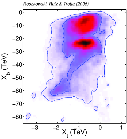
Figure 2: The 2–dim relative probability density in the plane of $X_{t}$ and $X_{b}$. The probability color code shown here applies also to all subsequent figures showing 2–dim relative probability density. The inner (outer) solid contours delimit the regions of 68% and 95% total probability, respectively.

3 Properties of the lightest Higgs boson in the CMSSM

In this work we are particularly interested in the properties of the lightest neutral Higgs boson. At the tree level, the Higgs sector of the MSSM is determined by $\tan\beta$ and $m_{A}$. The (by far dominant) one–loop radiative corrections are generated by diagrams involving the top quark and its scalar partners, and, at large $\tan\beta$, also the bottom quark and its scalar partners. Both are proportional to their respective Yukawa couplings. The radiative corrections have been computed using several different methods. Full one–loop expressions are known [33, 34, 35]. Leading two–loop corrections have been computed using renormalization group [36] and two–loop effective potential methods [37, 38], and in the Feynman–diagrammatic approach [39]. Furthermore the tadpole corrections, needed to minimise the effective scalar potential, have been calculated at one loop [35, 40] and the leading ones at two loops [41, 42]. The remaining theoretical uncertainty in the light Higgs mass $m_{h}$ has conservatively been estimated at $\mathrel{\hbox to0.0pt{\lower 4.0pt\hbox{\hskip 1.0pt$\sim$}\hss}\raise 1.0pt\hbox{$<$}}3\mbox{ GeV}$ [43, 44].

In computing the Higgs (and SUSY) mass spectrum we employ the code SOFTSUSY v2.08 [45], which implements radiative corrections in the modified Dimensional Reduction scheme, $\overline{DR}$, based on the results of [35, 38, 41]. For comparison, in FeynHiggs [46] the On–Shell scheme approach is adopted. Both are in good agreement [43], i.e., within the above theoretical uncertainty.

In the literature one often considers the cases of “maximal mixing” and “no mixing” (or “minimal mixing”) to describe the impact on the Higgs sector of the off–diagonal terms $m_{q}X_{q}$ ($q=t,b$) in the stop and sbottom mass matrices relative to their diagonal entries. In terms of

$$X_{t}=A_{t}-\mu\cot\beta,~{}~{}~{}~{}~{}~{}~{}~{}~{}~{}~{}~{}~{}~{}~{}~{}X_{b}=A_{b}-\mu\tan\beta,$$ (4)

where $A_{t,b}$ are the stop/sbottom trilinear soft parameters, the “no mixing” case, in particular, corresponds to $X_{t}=0$ and $X_{b}=0$. In fig. 1 we show in the left panel the 1–dim relative probability densities for $X_{t}$ and in the right panel those for $X_{b}$ in the CMSSM. Their 2–dim relative probability density (marginalized over all other parameters) is shown in fig. 2. One can see that both variables are typically negative, with $|X_{b}|\gg|X_{t}|$. Very large negative values of $X_{b}$ are predominantly caused by the fact that the relative probability density of $\tan\beta$ is strongly peaked at large values of $\simeq 52$ [9, 11, 19]; compare fig. 2 of [11]. Such large values of both $X_{t}$ and $X_{b}$ do not, however, necessarily imply large mixings in the stop and sbottom sectors since in the corresponding mass matrices they are multiplied by their respective quark masses. In fact, in the CMSSM in the sbottom sector we find a nearly strict no–mixing limit while in the stop sector we find a spread of values (mild mixing) but again with the peak in the probability distribution close to no mixing. Note that the ranges of $X_{t}$ and $X_{b}$ in figs. 1 and 2 are very different from the values proposed for general MSSM Higgs searches at the Tevatron [21, 22].

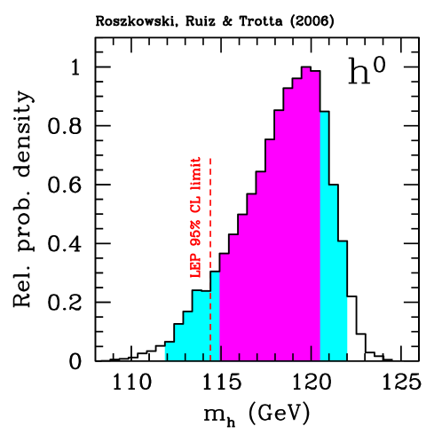
Figure 3: The 1–dim relative probability density for the light Higgs boson mass $m_{h}$. Magenta (dark shaded) and cyan (shaded) bands delimit 68% and 95% posterior probability (2 tails) ranges of $m_{h}$, respectively.

The values of $X_{t}$ and $X_{b}$ determine to some extent the upper bound on $m_{h}$ [1, 2]:

$$m_{h}^{2}\mathrel{\hbox to0.0pt{\lower 4.0pt\hbox{\hskip 1.0pt$\sim$}\hss}\raise 1.0pt\hbox{$<$}}m_{Z}^{2}+\frac{3g_{2}^{2}m_{t}^{4}}{8\pi^{2}m_{W}^{2}}\left[\mbox{ln}\left(\frac{{\overline{m}}_{{\widetilde{t}}}^{2}}{m_{t}^{2}}\right)+\frac{X_{t}^{2}}{{\overline{m}}_{{\widetilde{t}}}^{2}}\left(1-\frac{X_{t}^{2}}{12{\overline{m}}_{{\widetilde{t}}}^{2}}\right)\right]+\left(t\to b,{\widetilde{t}}\to{\widetilde{b}}\right),$$ (5)

where $g_{2}$ is the $SU(2)_{L}$ gauge coupling and ${\overline{m}}_{{\widetilde{t}}}^{2}=(m_{{\widetilde{t}}_{1}}^{2}+m_{{\widetilde{t}}_{2}}^{2})/2$ is an average stop mass–squared, and analogously for the sbottoms. From fig. 2 one can easily see that the bottom–sbottom contribution to (5) can be comparable to the top–stop one.

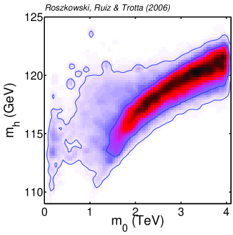
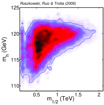
Figure 4: The 2–dim relative probability densities in the plane of $(m_{0},m_{h})$ (left panel) and $(m_{1/2},m_{h})$ (right panel). The inner (outer) solid contours delimit the regions of 68% and 95% total probability, respectively.

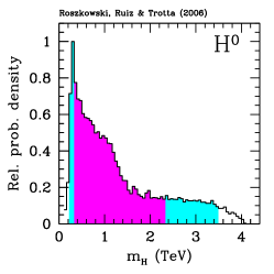
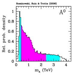
Figure 5: The 1–dim relative probability densities for the masses of $H$, $A$ and $H^{\pm}$, respectively. Magenta (dark shaded) and cyan (shaded) bands delimit mass ranges of 68% and 95% of posterior probability (2 tails), respectively.

In fig. 3 we display the 1–dim relative probability density of the light Higgs scalar mass. It is clearly well confined, with the ranges of posterior probability given by

$$115.4\mbox{ GeV}<m_{h}<120.4\mbox{ GeV} (68\%\text{ region}),$$ (6)

$$112.5\mbox{ GeV}<m_{h}<121.9\mbox{ GeV} (95\%\text{ region}).$$

The finite tail on the l.h.s. of the relative probability density in fig. 3, below the final LEP–II lower bound of $114.4\mbox{ GeV}$ (95% CL) is a consequence of the fact that our likelihood function does not simply cut off points with $m_{h}$ below some arbitrary CL, but instead it assigns to them a lower probability, as described above. On the other hand, the sharp drop–off on the r.h.s. of the relative probability density is mostly caused by the assumed upper bound on $m_{0}<4\mbox{ TeV}$. This is shown in the left panel of fig. 4. The upper bound on $m_{h}$ increases with ${\overline{m}}_{{\widetilde{t}}}$ and ${\overline{m}}_{{\widetilde{b}}}$ (5), whose largest values in turn depend on the maximum allowed value of $m_{0}$, as we could already see in fig. 5 of [11]. With the new SM value for $BR(\overline{B}\rightarrow X_{s}\gamma)$ in the current analysis, the dependence on the prior range of $m_{0}$ has, unfortunately, become even stronger. For instance, adopting a much more generous upper limit $m_{0}<8\mbox{ TeV}$ would lead to changing the ranges 6 to roughly $120.4\mbox{ GeV}\mathrel{\hbox to0.0pt{\lower 4.0pt\hbox{\hskip 1.0pt$\sim$}\hss}\raise 1.0pt\hbox{$<$}}m_{h}\mathrel{\hbox to0.0pt{\lower 4.0pt\hbox{\hskip 1.0pt$\sim$}\hss}\raise 1.0pt\hbox{$<$}}124.4\mbox{ GeV}$ (68% CL) and $115.4\mbox{ GeV}\mathrel{\hbox to0.0pt{\lower 4.0pt\hbox{\hskip 1.0pt$\sim$}\hss}\raise 1.0pt\hbox{$<$}}m_{h}\mathrel{\hbox to0.0pt{\lower 4.0pt\hbox{\hskip 1.0pt$\sim$}\hss}\raise 1.0pt\hbox{$<$}}125.6\mbox{ GeV}$ (95% CL). We will come back to this issue when we discuss light Higgs detection prospects at the Tevatron.

On the other hand, the upper bound on $m_{h}$ does not depend on the upper limit imposed in the prior for $m_{1/2}$, as can be seen in the right panel of fig. 4 (compare also fig. 2 in ref. [11]). Basically, for very large $\tan\beta\mathrel{\hbox to0.0pt{\lower 4.0pt\hbox{\hskip 1.0pt$\sim$}\hss}\raise 1.0pt\hbox{$>$}}60$ the bottom quark Yukawa running coupling becomes non–perturbative below the unification scale and it is no longer possible to find consistent mass spectra using the RGEs. This upper bound on $\tan\beta$ limits from above the values of $m_{1/2}$ that can still be consistent with $\Omega_{\chi}h^{2}$ [11].

Fig. 3 confirms the well–known fact that in the CMSSM the largest values of $m_{h}$ are typically much lower than in the general MSSM where stop and sbottom masses can to a large extent be treated as free parameters. The shape of the relative probability density also agrees rather well with ref. [12].

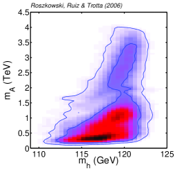
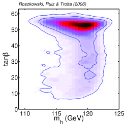
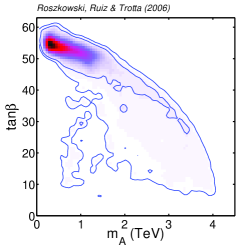
Figure 6: The 2–dim relative probability density in the plane of $(m_{h},m_{A})$ (left panel), $(m_{h},\tan\beta)$ (middle panel) and $(m_{A},\tan\beta)$ (right panel).

The other Higgs bosons are typically somewhat, but not necessarily much, heavier. This can be seen in fig. 5, where we show the 1–dim relative probability densities for the masses of $H$, $A$ and $H^{\pm}$, respectively. Note that the shapes of their relative probability densities are almost identical since the masses of the three Higgs bosons are nearly degenerate. Their posterior probability regions are given by

$$0.4\mbox{ TeV}<m_{H,A,H^{\pm}}<2.5\mbox{ TeV} (68\%\text{ region}),$$ (7)

$$0.2\mbox{ TeV}<m_{H,A,H^{\pm}}<3.6\mbox{ TeV} (95\%\text{ region}).$$

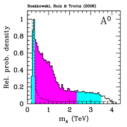
Figure 7: The same as in figs. 3 and 5 but with the mean quality–of–fit (dashed line) added for comparison.

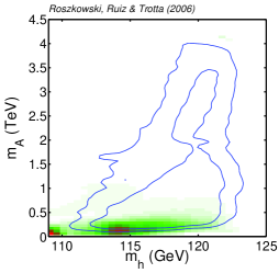
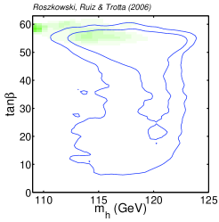
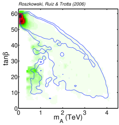
Figure 8: The mean quality–of–fit (dashed line) in the planes of $(m_{h},m_{A})$ (left panel), $(m_{h},\tan\beta)$ (middle panel) and $(m_{A},\tan\beta)$ (right panel). The 68% and 95% posterior probability contours from fig. 6 are also shown for comparison.

It is interesting to see a 2–dim relative probability density in the ($m_{h},m_{A}$) plane. This is presented in the left panel of fig. 6. One can see that the pseudoscalar mass $m_{A}$ always remains somewhat larger than $m_{h}$, but that most of its probability density is actually concentrated at fairly low values. (Compare also fig. 5.) For $m_{h}\mathrel{\hbox to0.0pt{\lower 4.0pt\hbox{\hskip 1.0pt$\sim$}\hss}\raise 1.0pt\hbox{$<$}}115\mbox{ GeV}$ (118 GeV), at 68% CL we find $m_{A}\mathrel{\hbox to0.0pt{\lower 4.0pt\hbox{\hskip 1.0pt$\sim$}\hss}\raise 1.0pt\hbox{$<$}}0.8\mbox{ TeV}$ (1.5 TeV). Experimental limits on Higgs boson searches in the MSSM are often presented in the plane spanned by the mass of the Higgs boson and $\tan\beta$. Our CMSSM results for the 2–dim relative probability density are presented in fig. 6 in the plane of $(m_{h},\tan\beta)$ (middle panel) and $(m_{A},\tan\beta)$ (right panel). It is clear from fig. 6 that in the CMSSM $m_{A}\gg m_{Z}$ (the decoupling regime) but we find $m_{A}$ predominantly in the regime of a few hundred GeV, which is on the borderline of a “mild decoupling” regime. This will affect some relevant Higgs couplings, as we will see shortly.

At this point we want to digress to emphasize the difference between posterior probability (Bayesian statistics) and the mean quality–of–fit statistics. In the absence of strong constraints from data, the two can produce quite different distributions, which ought to be interpreted carefully since their meaning is different. (See ref. [11] for more details and a thorough discussion.) We illustrate this in fig. 7, for the case of Higgs masses where we show the distribution of the mean quality–of–fit (dashed line) in addition to the relative probability density. Next, in fig. 8 we present the mean quality–of–fit in the planes of $(m_{h},m_{A})$ (left panel), $(m_{h},\tan\beta)$ (middle panel) and $(m_{A},\tan\beta)$ (right panel). This figure should be compared with fig. 6. It is clear that the largest values of the mean quality–of–fit show preference for a smaller $m_{h}$, with the peak of the distribution at $114\mbox{ GeV}$ (below the LEP–II bound of $114.4\mbox{ GeV}$). The mean quality–of–fit also favors significantly smaller $m_{A}\mathrel{\hbox to0.0pt{\lower 4.0pt\hbox{\hskip 1.0pt$\sim$}\hss}\raise 1.0pt\hbox{$<$}}1\mbox{ TeV}$ (as well as the other heavy Higgs masses). We note that, according to the mean quality–of–fit statistics, the favored region of parameter space lies at smaller masses than the 68% range of posterior probability, as can be seen in fig. 7. Such a discrepancy between the two statistical measures can only be resolved with better data. We also note that we have found a handful of points (about 100) with $\zeta_{h}^{2}\ll 1$ exhibiting a very good quality–of–fit at very small values of $m_{h}\sim 90\mbox{ GeV}$. Since their statistical weight is insignificant (compared to some $3\times 10^{5}$ samples in our chain) we do not display their quality–of–fit in fig. 8.

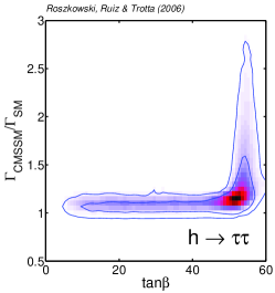
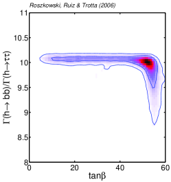
Figure 9: The 2–dim relative probability density in the plane of $\tan\beta$ and the decay width $\Gamma(h\to b\bar{b})_{\text{CMSSM}}$ (left panel) and $\Gamma(h\to\tau^{+}\tau^{-})_{\text{CMSSM}}$ (middle panel) in the CMSSM, both normalized to the SM values. In the right panel the same quantity is plotted for the ratio of the two widths. The inner (outer) solid contours encompass regions of the 68% (95%) total probability, respectively.

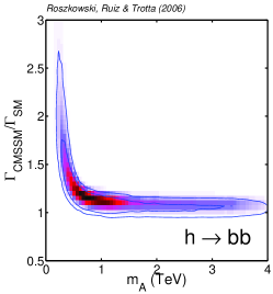
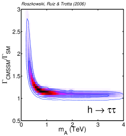
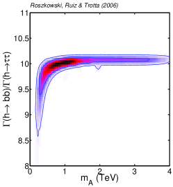
Figure 10: The same as in fig. 9 but with $\tan\beta$ replaced by $m_{A}$.

Next, we discuss some relevant couplings. We compute them with the help of FeynHiggs v2.5.1 [46] via the corresponding decay widths. For this purpose we translate all the Higgs and superpartner mass spectra and other relevant parameters from the output of SOFTSUSY. The decay widths of the neutral Higgs bosons are evaluated with the full rotation to on–shell Higgs bosons, i.e., beyond the effective coupling approximation. That means that the mixing matrix is constructed through the $Z$–factors resulting from the Higgs boson wave function normalization [48]. In the case of the vector bosons $V=Z,W$ the coupling ratio is $g(hVV)_{\text{MSSM}}/g(hVV)_{\text{SM}}=\sin(\beta-\alpha_{\text{eff}})$, where $\alpha_{\text{eff}}$ denotes the effective (i.e., radiatively–corrected) mixing angle in the Higgs scalar sector. The ratio is typically strongly suppressed in the general MSSM. In contrast, in the CMSSM it is close to 1 as we have already mentioned when discussing $\zeta_{h}^{2}$ in the previous section. This is the case in both the decoupling and the mild decoupling regimes.

The light Higgs couplings–squared to the third generation down–type fermions show a more complex behavior, as shown in figs. 9 and 10. In the (C)MSSM the light Higgs coupling to bottoms $g(hb\bar{b})_{\text{CMSSM}}$ and to taus $g(h\tau^{+}\tau^{-})_{\text{CMSSM}}$, normalized to their SM value, $g(hf\bar{f})_{\text{SM}}=gm_{b,\tau}/2m_{W}$, are given by $-\sin\alpha_{\text{eff}}/\cos\beta=\sin(\beta-\alpha_{\text{eff}})-\tan\beta\cos(\beta-\alpha_{\text{eff}})$. At tree level both ratios are equal to 1. We note two effects here. First, for not too large $\tan\beta\mathrel{\hbox to0.0pt{\lower 4.0pt\hbox{\hskip 1.0pt$\sim$}\hss}\raise 1.0pt\hbox{$<$}}45$ (for which in the CMSSM there is strong preference for $m_{A}\mathrel{\hbox to0.0pt{\lower 4.0pt\hbox{\hskip 1.0pt$\sim$}\hss}\raise 1.0pt\hbox{$>$}}1\mbox{ TeV}$) we find that the ratio $\Gamma_{\text{CMSSM}}/\Gamma_{\text{SM}}$ becomes close to 1.01. This is probably again just a result of an approximation used in FeynHiggs, as in the case of the $VV$ mode. At larger $\tan\beta$ the second term starts playing a bigger role. As $m_{A}$ decreases to below some $0.8\mbox{ TeV}$, corresponding to large $\tan\beta\mathrel{\hbox to0.0pt{\lower 4.0pt\hbox{\hskip 1.0pt$\sim$}\hss}\raise 1.0pt\hbox{$>$}}50$, both coupling–squared ratios grow rather fast. The enhancements in this region can be seen in the left and middle panels of figs. 9 and 10. At the $2\sigma$ level, we find that the widths are increased relative to their SM counterparts by a factor of up to some 2.5.

The second effect on the couplings is caused by radiative corrections from sbottom–gluino and stop–higgsino loops to the tree–level relation between the bottom mass and its Yukawa coupling [47]. At large $\tan\beta$ this leads to modifying the coupling $g(hb\bar{b})$ [49], while the analogous coupling to taus is not affected. (Implications of this effect for Tevatron Higgs searches have recently been discussed in ref. [22].) As a result, in the CMSSM at large $\tan\beta\mathrel{\hbox to0.0pt{\lower 4.0pt\hbox{\hskip 1.0pt$\sim$}\hss}\raise 1.0pt\hbox{$>$}}50$, in a sizable number of cases the quantity $g^{2}(hb\bar{b})_{\text{CMSSM}}$, while remaining dominant, will show a small decrease relative to $g^{2}(h\tau^{+}\tau^{-})_{\text{CMSSM}}$. This feature, which is displayed in the right panels of figs. 9 and 10, will give one some chance of producing a somewhat increased number of taus in light Higgs decays at the Tevatron, as we will see shortly.

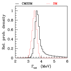
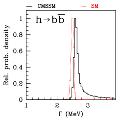
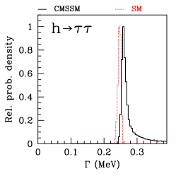
Figure 11: The 1–dim relative probability densities for the light Higgs total decay width (left panel) and partial decay widths to $b\bar{b}$ (middle panel) and $\tau^{+}\tau^{-}$ (right panel). For comparison, the widths of the SM Higgs boson with the same mass are also shown.

Figure 12: The 1–dim relative probability density of the branching ratios $BR(h\to b\bar{b})$ (left panel), $BR(h\to\tau^{+}\tau^{-})$ (middle panel) and $BR(h\to WW^{\ast})$ (right panel), all normalized to their SM counterparts.

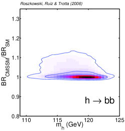
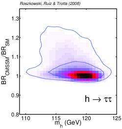
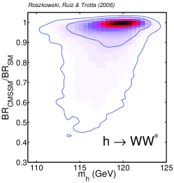
Figure 13: The 2–dim relative probability density of the branching ratios $BR(h\to b\bar{b})$ (left panel), $BR(h\to\tau^{+}\tau^{-})$ (middle panel) and $BR(h\to WW^{\ast})$ (right panel), all normalized to their SM counterparts, as a function of $m_{h}$.

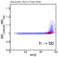
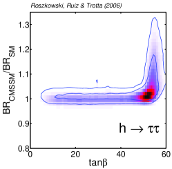
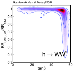
Figure 14: The 2–dim relative probability density of the branching ratios $BR(h\to b\bar{b})$ (left panel), $BR(h\to\tau^{+}\tau^{-})$ (middle panel) and $BR(h\to WW^{\ast})$ (right panel), all normalized to their SM counterparts, as a function of $\tan\beta$.

We will now examine the impact of the above properties of the light Higgs couplings on its decays. The varying of the couplings to bottoms and staus is reflected in the total and partial decay widths of $h$ to $b\bar{b}$ and $\tau^{+}\tau^{-}$ for which relative probability densities are presented in fig. 11. For comparison, we show the same quantities for the SM Higgs with the same mass. Somewhat larger widths in the $b\bar{b}$ and $\tau^{+}\tau^{-}$ modes are a result of both decay channels being enhanced at large $\tan\beta$. On the other hand, we have checked that the decay width for $h\to W^{\ast}W$ (followed by vector boson decays into light fermions) shows no deviation from the SM.

The ensuing effect on the branching ratios is shown in figs. 12–14. We remind the reader that, in the range of mass predicted in the CMSSM, the SM–like light Higgs boson decays predominantly into $b\bar{b}$ pairs ($\sim 90\%$), followed by $\tau^{+}\tau^{-}$ pairs ($\sim 9\%$), although at small $\tan\beta$ the $h\to WW^{\ast}$ branching ratio grows quickly with $m_{h}$ and at $m_{h}\simeq 120\mbox{ GeV}$ it can exceed some $10\%$ (at the expense of the above two channels). The dominance of the $b\bar{b}$ mode, however, is so large that, despite some decrease of the coupling $hb\bar{b}$ relative to the one of $h\tau^{+}\tau^{-}$ at large $\tan\beta$ in some parts of the CMSSM parameter space, the branching ratio into $b\bar{b}$ remains basically unaffected. On the other hand it is the subdominant modes $\tau^{+}\tau^{-}$ and $WW^{\ast}$ that, at large $\tan\beta$, can experience either a relative increase or decrease, respectively. These effects can be seen in fig. 12, where we display 1–dim relative pdf’s of the branching ratios for $h\to b\bar{b}$ (left panel), $h\to\tau^{+}\tau^{-}$ (middle panel) and $h\to WW^{\ast}$ (right panel), all normalized to the analogous quantities for the SM Higgs boson. The corresponding 2–dim relative probability densities are shown in figs. 13 and 14, in the planes spanned by the above SM–normalized branching ratios and $m_{h}$ and $\tan\beta$, respectively. Note a small increase in the number of produced $\tau$–leptons (which is rather small to start with), which may help in Higgs searches in that important decay channel.

In conclusion, in the CMSSM with flat prior ranges as given at the beginning of sec. 2.2 (most importantly $m_{0}<4\mbox{ TeV}$) and with observables as in tables 1 and 2, the mass of the light Higgs lies predominantly in the range shown in (6) and fig. 3, while the other Higgs bosons are typically somewhat, but not necessarily much, heavier. The light Higgs coupling to $VV$ remains basically SM–like, while the ones to $b\bar{b}$ and $\tau^{+}\tau^{-}$ do show some increase relative to the SM ones at large $\tan\beta$. This has some effect on on light Higgs decays and, in the case of the bottoms, also on its production, as we shall see in the next section.

4 Light Higgs production and decay

We will now assess the discovery prospects of the light CMSSM Higgs boson at the Tevatron. To this end we will consider the following production and decay processes:

• vector boson bremsstrahlung: $V^{\ast}\to Vh$ (where $V=W,Z$), followed by $h\to b\bar{b}$, $h\to\tau^{+}\tau^{-}$ or, in the case of $Wh$, also $h\to WW^{\ast}$;

• gluon–gluon fusion: $gg\to h$, followed by either $h\to WW^{\ast}$ or $h\to\tau^{+}\tau^{-}$;

• associated bottom production: $hb(b)$, with a $b$ quark tagged on a hard spectrum ($p_{T}>15\mbox{ GeV}$ and $\eta<2.5$), followed by either $h\to b\bar{b}$ or $h\to\tau^{+}\tau^{-}$;

• inclusive production: $p\bar{p}\to h$, followed by $h\to\tau^{+}\tau^{-}$.

We have also considered $VV$ fusion and $t\bar{t}h$ Higgs production processes, but in the CMSSM these are subdominant.

Some additional comments about the processes that we consider are in order. The vector boson bremsstrahlung process is determined by the effective coupling $g(hVV)\sim\sin(\beta-\alpha_{\text{eff}})$. On the other hand, the other three processes are to a large extent determined by the behavior of the effective coupling $g(hb\bar{b})$ which, as we have seen above, for $\tan\beta\mathrel{\hbox to0.0pt{\lower 4.0pt\hbox{\hskip 1.0pt$\sim$}\hss}\raise 1.0pt\hbox{$>$}}50$ and $m_{A}\mathrel{\hbox to0.0pt{\lower 4.0pt\hbox{\hskip 1.0pt$\sim$}\hss}\raise 1.0pt\hbox{$<$}}1\mbox{ TeV}$, can markedly deviate from the SM value.

In the gluon–gluon fusion process $gg\to h$ we include diagrams with top or bottom quark (and their superpartner) lines in the loop. In the associated bottom production process $hb(b)$ we compute the cross section of $bg\to bh$. An alternative, and effectively equivalent, way would be to consider the process $gg\to hb\bar{b}$ with the momentum of one of the bottoms integrated out [50]. The inclusive process $p\bar{p}\to h$ can likewise be computed in two ways. At NLO in the four–flavor scheme one can add the (dominant) process $gg\to hb\bar{b}$ and the (subdominant) one $q\bar{q}\to hb\bar{b}$, and integrate out the momenta of the bottoms. Alternatively, one obtains very similar results by computing the process $b\bar{b}\to h$ at NNLO in the five–flavor scheme [50]. Here we follow the latter approach. Relative strengths of the above processes depend on several parameters, especially on $\tan\beta$ (when large) but typically, in the MSSM in the regime of light Higgs mass and large $\tan\beta$, the gluon–gluon fusion process is dominant and associated bottom production is a factor of a few smaller but otherwise comparable. For a comprehensive review of Higgs properties and collider search prospects, see, for instance, ref. [2].

Since, as we have seen above, the light Higgs boson is SM–like, it will be convenient to normalize our results to the corresponding processes involving the SM Higgs boson with the same mass. We expect most ratios to be close to 1 and in fact it is some possible departures from the SM case that we will attempt to identify.

We compute the light Higgs production cross sections in the CMSSM, normalized to their SM counterparts, $\sigma_{\text{CMSSM}}/\sigma_{\text{SM}}$, with the help of FeynHiggs v2.5.1 [46]. The package implements the Higgs production cross sections at the Tevatron and the LHC, both evaluated in the effective coupling approximation using the SM cross sections provided in ref. [51]. The calculation of the branching ratios is based on ref. [52]. The code also includes SUSY corrections to Higgs couplings to the bottom quarks, which can be substantial at large $\tan\beta$, as discussed earlier.

Figure 15: The 1–dim relative probability density for light Higgs production cross sections at the Tevatron (normalized to the SM case) for $V^{\ast}\to Vh$, where $V=Z,W$ (upper left panel), $gg\to h$ (upper right panel), $hb(b)$ (lower left panel) and $p\bar{p}\to h$ (lower right panel).

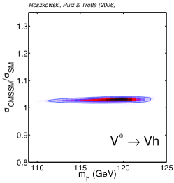
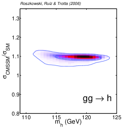
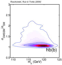
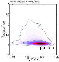
Figure 16: The 2–dim relative probability density of light Higgs production cross sections at the Tevatron (normalized to the SM case) as a function of its mass $m_{h}$.

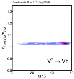
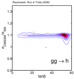
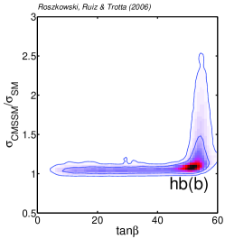
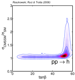
Figure 17: The 2–dim relative probability density for light Higgs production cross sections at the Tevatron (normalized to the SM case) as a function of $\tan\beta$.

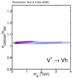
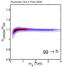
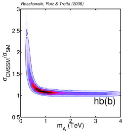
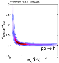
Figure 18: The 2–dim relative probability density for light Higgs production cross sections at the Tevatron (normalized to the SM case) as a function of $m_{A}$.

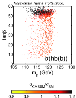
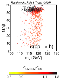
Figure 19: Values in the $(m_{h},\tan\beta)$ plane of light Higgs production cross sections at the Tevatron (normalized to the SM case) for the processes $hb(b)$ and $p\bar{p}\to h$. For the processes $V^{\ast}\to Vh$, where $V=Z,W$, and $gg\to h$ the values are almost independent of $\tan\beta$; compare fig. 17.

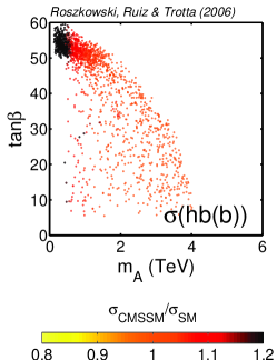
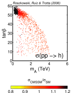
Figure 20: Values in the $(m_{A},\tan\beta)$ plane of light Higgs production cross sections at the Tevatron (normalized to the SM case) for the processes $hb(b)$ and $p\bar{p}\to h$. For the processes $V^{\ast}\to Vh$, where $V=Z,W$, and $gg\to h$ the values are almost independent of $\tan\beta$ and $m_{A}$; compare figs. 17 and 18.

As above, we will follow the procedure developed in [11] in presenting our results in terms of relative posterior pdf, here simply called relative probability density, for various variables. First, in fig. 15 we display relative probability densities for $\sigma_{\text{CMSSM}}/\sigma_{\text{SM}}$ for the processes of primary interest at the Tevatron. All the ratios are close to 1 but only in the case of $V^{\ast}\to Vh$ ($V=Z,W$) is a pdf very strongly peaked very close to 1. The pdf for the gluon–gluon fusion SM–normalized cross section is peaked around 1.1, with rather little variation. This is a reflection of the behavior of the (radiatively corrected) coupling $g(hb\bar{b})_{\text{CMSSM}}$; compare the left panels of figs. 9 and 10. For the remaining two processes we observe some more variation, and increase relative to the SM, than in $gg\to h$. Actually, because of the way these processes are computed (as described above), their pdf’s will in most cases be very similar. We nevertheless present them both for completeness.

In order to display the behavior of the production cross sections in more detail, we present in fig. 16 a 2–dim relative probability density of the SM–normalized cross sections as a function of $m_{h}$, in fig. 17 of $\tan\beta$ and in fig. 18 of the pseudoscalar Higgs mass $m_{A}$. As regards the gluon–gluon fusion process, the bottom quark exchange contribution to the cross section is subdominant relative to the top quark one (by a factor of a few). This explains why there is much less variation in the corresponding pdf than for $hb(b)$ and $p\bar{p}\to h$. On the other hand, the enhancement of the coupling $g(hb\bar{b})_{\text{CMSSM}}$ at $\tan\beta\mathrel{\hbox to0.0pt{\lower 4.0pt\hbox{\hskip 1.0pt$\sim$}\hss}\raise 1.0pt\hbox{$>$}}50$ and $m_{A}\mathrel{\hbox to0.0pt{\lower 4.0pt\hbox{\hskip 1.0pt$\sim$}\hss}\raise 1.0pt\hbox{$<$}}1\mbox{ TeV}$, cause a slight increase of a few per cent in the cross section relative to the SM. Otherwise, unsurprisingly, the pdf’s for the three processes mirror the behavior of the $g(hb\bar{b})_{\text{CMSSM}}$ coupling and we include them for completeness. To finish our discussion of light Higgs production, we present in fig. 19 the ranges in the CMSSM of the SM–normalized cross sections for the above two processes in the plane of $\tan\beta$ and $m_{h}$, while in fig. 20 the same is shown in the plane of $\tan\beta$ and $m_{A}$.

Figure 21: The 1–dim relative probability density for light Higgs production cross sections times decay branching ratios at the Tevatron (normalized to the SM case).

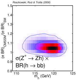
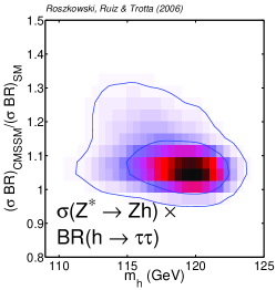
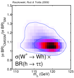
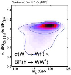
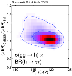
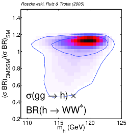
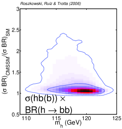
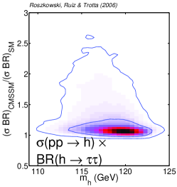
Figure 22: The 2–dim relative probability density of light Higgs production cross sections times decay branching ratios at the Tevatron (normalized to the SM case) as a function of its mass $m_{h}$.

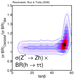
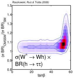
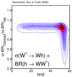
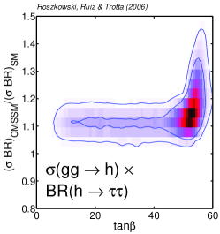
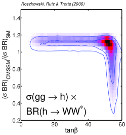
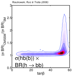
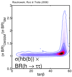
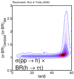
Figure 23: The 2–dim relative probability density for light Higgs production cross sections times decay branching ratios at the Tevatron (normalized to the SM case) as a function of $\tan\beta$.

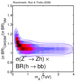
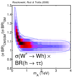
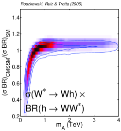
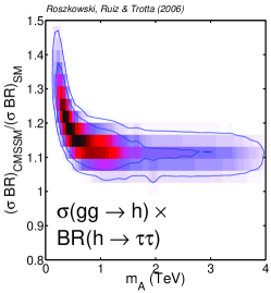
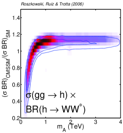
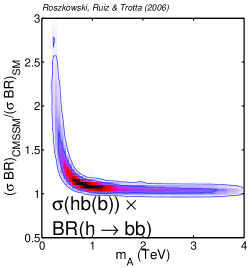
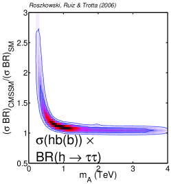
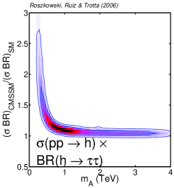
Figure 24: The 2–dim relative probability density for light Higgs production cross sections times decay branching ratios at the Tevatron (normalized to the SM case) as a function of $m_{A}$.

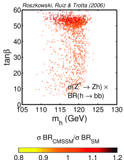
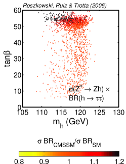
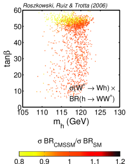
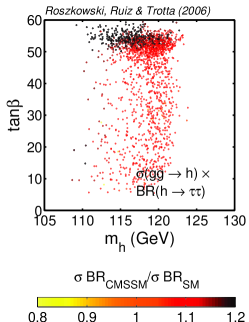
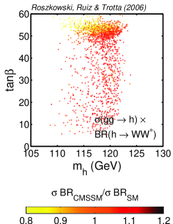
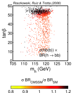
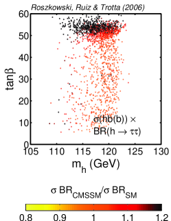
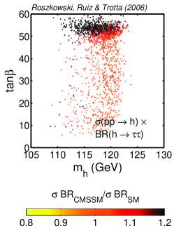
Figure 25: Values in the $(m_{h},\tan\beta)$ plane of production cross section times the branching ratio, normalized to their SM values, for the main light CMSSM Higgs production and decay channels at the Tevatron in the $(m_{h},\tan\beta)$ plane.

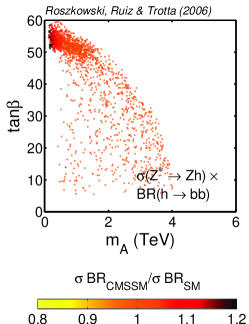
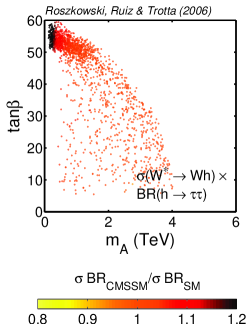
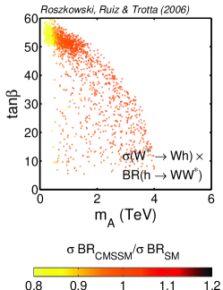
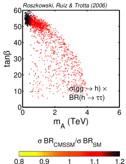
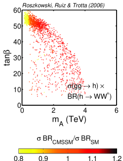
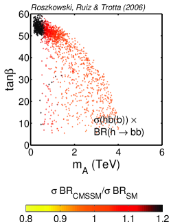
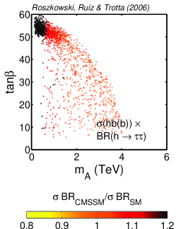
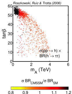
Figure 26: Values in the $(m_{A},\tan\beta)$ plane of production cross section times the branching ratio, normalized to their SM values, for the main light CMSSM Higgs production and decay channels at the Tevatron.

We now combine the above results for the light Higgs production cross sections and decay branching ratios at the Tevatron. In fig. 21 we show 1–dim relative probability densities for SM–normalized light Higgs production cross section times decay branching ratio $(\sigma\times BR)_{\text{CMSSM}}/(\sigma\times BR)_{\text{SM}}$, while the ratio’s dependence on $m_{h}$ is displayed in fig. 22, on $\tan\beta$ in fig. 23, and on $m_{A}$ in fig. 24. In fig. 25 we show a distribution of values of the above product in the plane spanned by $m_{h}$ and $\tan\beta$, while in fig. 26 the same quantities are shown in the usual plane of $m_{A}$ and $\tan\beta$. As before, all parameters other than the ones shown in each figure have been marginalized over.

The emerging picture is rather clear. As expected, in the CMSSM, for all the considered processes, we generally find very similar light Higgs search prospects as for the SM Higgs boson with the same mass. We note, however, some differences, which may help optimize search strategies. To start with, in the vector boson bremsstrahlung process $V^{\ast}\to Vh$ ($V=Z,W$), $h\to b\bar{b},\tau^{+}\tau^{-}$ modes are almost indistinguishable from the SM Higgs case with the same mass. This is caused by the fact that in the CMSSM the coupling $g(hVV)_{\text{CMSSM}}$ is very close to its SM value. We note, however, that we do find a slight enhancement of the $b\bar{b}$ and $\tau^{+}\tau^{-}$ final states, which may be of some help in these important search channels. The same is of course true for all the other processes considered here. On the other hand, we have found in the CMSSM parameter space some deviations in the $g(hb\bar{b})_{\text{CMSSM}}$ coupling from the SM value, which may significantly change production cross section of all the modes except $V^{\ast}\to Vh$. On the other hand, the $h\to WW^{\ast}$ mode is typically reduced by up to some 5% within the 68% posterior probability region. Within the 95% posterior probability region, it can actually be significantly reduced, especially in the region of $\tan\beta\mathrel{\hbox to0.0pt{\lower 4.0pt\hbox{\hskip 1.0pt$\sim$}\hss}\raise 1.0pt\hbox{$>$}}50$ and $m_{A}\mathrel{\hbox to0.0pt{\lower 4.0pt\hbox{\hskip 1.0pt$\sim$}\hss}\raise 1.0pt\hbox{$<$}}1\mbox{ TeV}$.

We emphasize that the results presented in figs. 21–26 have been derived in the framework of the CMSSM. This should be kept in mind when comparing them with existing experimental Higgs search limits. Many of them have been set for specific (e.g., maximal and no mixing) scenarios and/or choices of parameters in the general MSSM, which are basically never realized in the CMSSM. Conversely, it would be helpful to add to experimental results limits applicable to the CMSSM.

5 Summary and conclusions

In this work we have performed a global scan of the CMSSM parameter space by employing a powerful MCMC technique. We have then analyzed our results for light Higgs properties and discovery prospects at the Tevatron, mostly in terms of Bayesian statistics, although we have demonstrated that an alternative mean quality–of–fit analysis can lead to rather different results. In particular, while the former favors the light Higgs mass range above the final LEP–II 95% CL, the latter points more towards values below it for a large part.

The couplings of the light Higgs of the CMSSM to vector bosons and bottoms and taus are basically very similar to those of the SM Higgs boson with the same mass. Small enhancements, at the level of a few per cent, have been found in most of the CMSSM parameter space, although at large $\tan\beta\mathrel{\hbox to0.0pt{\lower 4.0pt\hbox{\hskip 1.0pt$\sim$}\hss}\raise 1.0pt\hbox{$>$}}50$ and $m_{A}\mathrel{\hbox to0.0pt{\lower 4.0pt\hbox{\hskip 1.0pt$\sim$}\hss}\raise 1.0pt\hbox{$<$}}1\mbox{ TeV}$ (the preferred region), the differences can be substantial. Our intention was to provide experimentalists involved in Higgs searches at the Tevatron detailed information about detection prospects of the CMSSM light Higgs boson. Despite the fact that the pdf’s for associate bottom production and inclusive Higgs production modes are basically indistinguishable, we have displayed them separately for the sake of completeness and convenience.

At the Tevatron, the sensitivity to a SM–like Higgs boson in the mass range of up to some $122\mbox{ GeV}$ (compare (6)) seems excellent. According to ref. [53], with about $2\,\mbox{fb}^{-1}$ of integrated luminosity per experiment (expected by the end of 2006), a 95% CL exclusion limit can be set for the whole 95% posterior probability light Higgs mass range given *** in (6) ****. We stress again that this conclusion depends on our assumed ranges of flat priors, especially on $m_{0}<4\mbox{ TeV}$, as discussed in the text. (Extending the range of $m_{0}$ up to $8\mbox{ TeV}$, and accordingly $m_{h}$ up to $\mathrel{\hbox to0.0pt{\lower 4.0pt\hbox{\hskip 1.0pt$\sim$}\hss}\raise 1.0pt\hbox{$<$}}125.6\mbox{ GeV}$ (95% CL), would require instead about $2.5\,\mbox{fb}^{-1}$ of integrated luminosity per experiment, which is again well within Tevatron’s reach.) While keeping this in mind, we still find it remarkable that negative Higgs searches at the Tevatron should allow one to make definitive conclusions about the ranges of CMSSM parameters, in particular $m_{0}$, which extend well beyond the reach of even the LHC in direct searches for superpartners.

Should a signal (hopefully) start being seen in this mass range, a $3\sigma$ evidence ($5\sigma$ discovery) can be claimed with about $4\,\mbox{fb}^{-1}$ ($12\,\mbox{fb}^{-1}$) per experiment. On the other hand, with about $8\,\mbox{fb}^{-1}$ of integrated luminosity ultimately expected per experiment, a $5\sigma$ discovery will be possible, should the light Higgs mass be around $115\mbox{ GeV}$. While such low mass is just below the 68% region of posterior probability according to Bayesian statistics, it is actually favored by an alternative mean quality–of–fit analysis. In other words, according to this measure, light Higgs search appears more promising than in the more conservative Bayesian probability scenario. A conclusive search for the CMSSM light Higgs boson at the Tevatron seems therefore fully feasible.

Acknowledgements
L.R. thanks the Theoretical Astrophysics Group at Fermilab and the CERN Theory Division for hospitality and support during his visits when some of the work was done. L.R. is grateful to P. Slavich, A. Sopczak and D. Tovey for helpful comments, and to A. Anastassov, G. Bernardi, T. Junk, J. Nachtman, S.M. Wang and T. Wright for their clarifications regarding Higgs searches at the Tevatron. R.RdA. thanks S. Heinemeyer and T. Hahn for their help with FeynHiggs and A.L. Read for providing LEP–II Higgs mass bounds data. We thank M. Misiak for providing us with his code and helpful information. R.T. thanks L. Lyons and G. Nicholls for useful discussions. R.RdA. is supported by the program “Juan de la Cierva” of the Ministerio de Educación y Ciencia of Spain. R.T. is supported by the Royal Astronomical Society through the Norman Lockyer Fellowship. R.T. thanks the Galileo Galilei Institute for Theoretical Physics for hospitality during the completion of this work and the INFN for partial support. We acknowledge support from ENTApP, part of ILIAS, contract number RII3-CT-2004-506222. L.R. acknowledges support from the EC 6th Framework Programme MRTN-CT-2004-503369. The use of the Glamdring cluster of Oxford University and the HEP cluster of Sheffield University are gratefully acknowledged. Parts of our numerical code are based on the publicly available package cosmomc.

References

- [1] M. Carena and H. E. Haber, Higgs Boson Theory and Phenomenology, Prog. Part. Nucl. Phys. 50 (2003) 63 [hep-ph/0208209] and references therein.
- [2] A. Djouadi, The anatomy of electro–weak symmetry breaking. II: The Higgs bosons in the minimal supersymmetric standard model, hep-ph/0503173 and references therein.
- [3] G. L. Kane, C. F. Kolda, L. Roszkowski and J. D. Wells, Study of constrained minimal supersymmetry, Phys. Rev. D49 (1994) 6173 [hep-ph/9312272].
-
[4]
See, e.g., H. P. Nilles,
Supersymmetry, Supergravity and Particle Physics,
Phys. Rep. 110 (1984) 1;
A. Brignole, L. E. Ibañez and C. Muñoz, Soft supersymmetry breaking terms from supergravity and superstring models, published in Perspectives on Supersymmetry, ed. G. L. Kane, 125 [hep-ph/9707209]. -
[5]
J. Ellis, S. Heinemeyer, K. A. Olive and G. Weiglein,
Observability of the lightest CMSSM Higgs boson at
hadron colliders, Phys. Lett. B515 (2001) 348 [hep-ph/0105061]; and
Precision analysis of the lightest Higgs boson at
future colliders, 2003006 [hep-ph/0211206]
;
S. Ambrosiano, A. Dedes, S. Heinemeyer, S. Su and G. Weiglein, Implications of the Higgs boson searches on different soft SUSY–breaking scenarios, Nucl. Phys. B624 (2002) 3 [hep-ph/0106255];
A. Dedes, S. Heinemeyer, S. Su and G. Weiglein, The Lightest Higgs boson of mSUGRA, mGMSB and mAMSB at present and future colliders: observability and precision analysis, Nucl. Phys. B674 (2003) 271 [hep-ph/0302174]. - [6] J. R. Ellis, S. Heinemeyer, K. A. Olive and G. Weiglein, Indirect sensitivities to the scale of supersymmetry, 2005013 [hep-ph/0411216].
- [7] See, e.g., B. A. Berg, Markov chain monte carlo simulations and their statistical analysis, World Scientific, Singapore (2004).
- [8] E. A. Baltz and P. Gondolo, Markov chain monte carlo exploration of minimal supergravity with implications for dark matter, 2004052 [hep-ph/0407039].
- [9] B. C. Allanach and C. G. Lester, Multi–dimensional MSUGRA likelihood maps, Phys. Rev. D73 (2006) 015013 [hep-ph/0507283].
- [10] B. C. Allanach, Naturalness priors and fits to the constrained minimal supersymmetric standard model, Phys. Lett. B635 (2006) 123 [hep-ph/0601089].
- [11] R. Ruiz de Austri, R. Trotta and L. Roszkowski, A Markov Chain Monte Carlo analysis of the CMSSM, 2006002 [hep-ph/0602028]; see also R. Trotta, R. Ruiz de Austri and L. Roszkowski, Prospects for direct dark matter detection in the Constrained MSSM, astro-ph/0609126.
- [12] B. C. Allanach, C. G. Lester and A. M. Weber, The dark side of mSUGRA, hep-ph/0609295.
- [13] J. Ellis, S. Heinemeyer, K. A. Olive and G. Weiglein, Phenomenological indications of the scale of supersymmetry, 2006005 [hep-ph/0602220].
- [14] P. Gambino and M. Misiak, Quark mass effects in , Nucl. Phys. B611 (2001) 338 [arXiv:hep-ph/0104034].
- [15] M. Misiak and M. Steinhauser, NNLO QCD corrections to the matrix elements using interpolation in , Nucl. Phys. B764 (2007) 62 [hep-ph/0609241].
- [16] T. Becher and M. Neubert, Analysis of at NNLO with a Cut on Photon Energy, Phys. Rev. Lett. 982007022003 [hep-ph/0610067].
- [17] E. Barberio et al. [HFAG], Averages of b-hadron properties at the end of 2005, hep-ex/0603003.
- [18] The CDF Collaboration, Observation of oscillations, hep-ex/0609040 and Measurement of the oscillation frequency, Phys. Rev. Lett. B97 (2006) 062003 [hep-ex/0606027].
- [19] L. Roszkowski, R. Ruiz de Austri and R. Trotta, in preparation.
-
[20]
A. Anastassov (for CDF and D0
Collaborations), Search for MSSM Higgs bosons at the Tevatron,
PoS HEP2005, 326 (2006).
See also, e.g., S. Choi, http://octs.osu.edu/PASCOS06/images/progsched/Sunday/choi.pdf for a recent presentation at PASCOS-2006. - [21] M. Carena, S. Heinemeyer, C. E. M. Wagner and G. Weiglein, Suggestions for benchmark scenarios for MSSM Higgs boson searches at hadron colliders, Eur. Phys. J. C26 (2003) 601 [hep-ph/0202167].
- [22] M. Carena, S. Heinemeyer, C. E. M. Wagner and G. Weiglein, MSSM Higgs boson searches at the Tevatron and the LHC: Impact of different benchmark scenarios, Eur. Phys. J. C45 (2006) 797 [hep-ph/0511023].
- [23] The Tevatron Electroweak Working Group, Combination of CDF and D0 results on the mass of the top quark, hep-ex/0608032.
- [24] W.-M. Yao et al. [Particle Data Group], J. Phys. G33 (2006) 1.
- [25] See http://lepewwg.web.cern.ch/LEPEWWG.
- [26] D.N. Spergel et al. [The WMAP Collaboration], Wilkinson Microwave Anisotropy Probe (WMAP) Three Year Results: Implications for Cosmology, astro-ph/0603449.
- [27] The CDF Collaboration, Search for and decays in collisions with CDF–II, CDF note 8176 (June 2006).
-
[28]
The LEP Higgs Working Group,
http://lephiggs.web.cern.ch/LEPHIGGS;
G. Abbiendi et al. [the ALEPH Collaboration, the DELPHI Collaboration, the L3 Collaboration and the OPAL Collaboration, The LEP Working Group for Higgs Boson Searches], Search for the standard model Higgs boson at LEP, Phys. Lett. B565 (2003) 61 [hep-ex/0306033]. - [29] J. Foster, K. Okumura and L. Roszkowski, Probing the flavour structure of supersymmetry breaking with rare B–processes: a beyond leading order analysis, 2005094 [hep-ph/0506146]; and Current and future limits on general flavour violation in b s transitions in minimal supersymmetry, 2006044 [hep-ph/0510422].
- [30] J. Foster, K. Okumura and L. Roszkowski, New Constraints on SUSY Flavour Mixing in Light of Recent Measurements at the Tevatron, Phys. Lett. B641 (2006) 452.
- [31] M. Awramik, M. Czakon, A. Freitas and G. Weiglein, Precise prediction for the W boson mass in the standard model, Phys. Rev. D69 (2004) 053006 [hep-ph/0311148]; and Complete two–loop electroweak fermionic corrections to and indirect determination of the Higgs boson mass, Phys. Rev. Lett. B93 (2004) 201805 [hep-ph/0407317].
- [32] A. Djouadi, P. Gambino, S. Heinemeyer, W. Hollik, C. Junger and G. Weiglein, Leading QCD corrections to scalar quark contributions to electroweak precision observables, Phys. Rev. D57 (1998) 4179 [hep-ph/9710438].
-
[33]
Y. Okada, M. Yamaguchi and T. Yanagida,
Upper bound of the lightest Higgs boson mass in the minimal
supersymmetric standard model, Prog. Theor. Phys. 85 (1991) 1;
J. Ellis, G. Ridolfi and F. Zwirner, Radiative corrections to the masses of supersymmetric Higgs bosons, Phys. Lett. B257 (1991) 83;
H. Haber and R. Hempfling, Can the mass of the lightest Higgs boson of the minimal supersymmetric model be larger than ?, Phys. Rev. Lett. B66 (1991) 1815. -
[34]
P. H. Chankowski, P. Pokorski and J. Rosiek,
Charged and neutral supersymmetric Higgs boson
masses: complete one loop analysis, Phys. Rev. Lett. B274 (1992) 191;
A. Brignole, Radiative corrections to the supersymmetric neutral Higgs boson masses, Phys. Lett. B281 (1992) 284;
A. Dabelstein, The one loop renormalization of the MSSM Higgs sector and its applications to the neutral scalar Higgs masses, Z. Phys. C67 (1995) 495 [hep-ph/9409375]. - [35] D. M. Pierce, J. A. Bagger, K. T. Matchev and R-J. Zhang, Precision corrections in the minimal supersymmetric standard model, Nucl. Phys. B491 (1997) 3 [hep-ph/9606211].
-
[36]
M. Carena, J. R. Espinosa, M. Quirós and C. E. M. Wagner,
Analytical expressions for radiatively corrected Higgs
masses and couplings in the MSSM,
Phys. Lett. B355 (1995) 209 [hep-ph/9504316];
M. Carena, M. Quirós and C. E. M. Wagner, Effective potential methods and the Higgs mass spectrum in the MSSM, Nucl. Phys. B461 (1996) 461 [hep-ph/9508343];
H. E. Haber, R. Hempfling and A. H. Hoang, Approximating the radiatively corrected Higgs mass in the minimal supersymmetric model, Z. Phys. C75 (1997) 539 [hep-ph/9609331]. -
[37]
R. Hempfling and A. H. Hoang,
Two loop radiative corrections to the upper limit of the
lightest Higgs boson mass in the minimal supersymmetric model,
Phys. Lett. B331 (1994) 99 [hep-ph/9401219];
J. R. Espinosa and R. J. Zhang, Complete two loop dominant corrections to the mass of the lightest CP even Higgs boson in the minimal supersymmetric standard model, Nucl. Phys. B586 (2000) 3 [hep-ph/0003246];
A. Brignole, G. Degrassi, P. Slavich and F. Zwirner, On the two loop sbottom corrections to the neutral Higgs boson masses in the MSSM, Nucl. Phys. B643 (2002) 79 [hep-ph/0206101];
A. Dedes, G. Degrassi and P. Slavich, On the two loop corrections to the neutral Higgs boson masses at large , Nucl. Phys. B672 (2003) 144 [hep-ph/0305127]. -
[38]
G. Degrassi, P. Slavich and F. Zwirner,
On the neutral Higgs boson masses in the MSSM for arbitrary
stop mixing, Nucl. Phys. B403 (2001) 403 [hep-ph/0105096];
A. Brignole, G. Degrassi, P. Slavich and F. Zwirner, On the two loop corrections to the neutral Higgs boson masses in the MSSM, Nucl. Phys. B631 (2002) 195 [hep-ph/0112177]. - [39] S. Heinemeyer, W. Hollik and G. Weiglein, The masses of the neutral CP even Higgs bosons in the MSSM: accurate analysis at the two loop level, Eur. Phys. J. C9 (1999) 343 [hep-ph/9812472]; The mass of the lightest MSSM Higgs boson: a compact analytical expression at two loop level, Phys. Lett. B455 (1999) 179 [hep-ph/9903404]; and Precise prediction for the mass of the lightest Higgs boson in the MSSM, Phys. Lett. B440 (1998) 296 [hep-ph/9807423].
-
[40]
P. Nath and R. Arnowitt,
Loop corrections to radiative breaking of electroweak symmetry
in supersymmetry, Phys. Rev. D46 (1992) 3981;
V. D. Barger, M. S. Berger and P. Ohmann, The supersymmetric particle spectrum, Phys. Rev. D49 (1994) 4908 [hep-ph/9311269]. - [41] A. Dedes and P. Slavich, Two loop corrections to radiative electroweak symmetry breaking in the MSSM, Nucl. Phys. B657 (2003) 333 [hep-ph/0212132].
- [42] S. P. Martin, Complete two loop effective potential aproximation to the lightest Higgs scalar boson mass in supersymmetry, Phys. Rev. D67 (2003) 095012 [hep-ph/0211366].
- [43] B. C. Allanach, A. Djouadi, J. L. Kneur, W. Porod and P. Slavich, Precise determination of the neutral Higgs boson masses in the MSSM, 2004044 [hep-ph/0406166].
- [44] S. Heinemeyer, W. Hollik, H. Rzehak and G. Weiglein, High-precision predictions for the MSSM Higgs sector at , Eur. Phys. J. C39 (2005) 465 [hep-ph/0411114].
- [45] B. C. Allanach, SOFTSUSY: a C++ program for calculating supersymmetric spectra, Comp. Phys. Comm. C143 (2002) 305 [hep-ph/0104145].
- [46] S. Heinemeyer, W. Hollik and G. Weiglein, Feynhiggs: a program for the calculation of the masses of the neutral CP even Higgs boson in the MSSM, Comp. Phys. Comm. C124 (2000) 76 [hep-ph/9812320].
-
[47]
T. Banks,
Supersymmetry and the quark mass matrix,
Nucl. Phys. B303 (1988) 172;
R. Hempfling, Yukawa coupling unification with supersymmetric threshold corrections, Phys. Rev. D49 (1994) 49;
L. J. Hall, R. Rattazzi and U. Sarid, The top quark mass in supersymmetric SO(10) unification, Phys. Rev. D50 (1994) 7048 [hep-ph/9306309];
M. Carena, M. Olechowski, S. Pokorski and C. E. M. Wagner, Electroweak symmetry breaking and bottom–top Yukawa unification, Nucl. Phys. B426 (1994) 269 [hep-ph/9402253]. - [48] M. Frank, T. Hahn, S. Heinemeyer, W. Hollik, H. Rzehak and G. Weiglein, The Higgs Boson Masses and Mixings of the Complex MSSM in the Feynman-Diagrammatic Approach, hep-ph/0611326.
- [49] M. Carena, D. Garcia, U. Nierste and C. E. M. Wagner, Effective Lagrangian for the interaction in the MSSM and charged Higgs phenomenology, Nucl. Phys. B577 (2000) 88 [hep-ph/9912516].
- [50] K. A. Assamagan et al., The Higgs working group: Summary report 2003, in Proceedings 3rd Les Houches Workshop: Physics at TeV Colliders, Les Houches, France, 26 May - 6 June 2003 [hep-ph/0406152].
- [51] TeV4LHC Higgs Working Group, http://maltoni.home.cern.ch/maltoni/TeV4LHC.
- [52] S. Heinemeyer, W. Hollik and G. Weiglein, Decay widths of the neutral CP even MSSM Higgs bosons in the Feynman diagrammatic approach, Eur. Phys. J. C16 (2000) 139 [hep-ph/0003022].
-
[53]
M. Carena, J. S. Conway, H. E. Haber and J. D. Hobbs,
Report of the Tevatron Higgs working group,
hep-ph/0010338;
L. Babukhadi et al. [CDF and D0 Working Group Members], Results of the Tevatron Higgs sensitivity study, FERMILAB-PUB-03-320-E, Oct 2003.