Strongly coupled plasma with electric and magnetic charges

Abstract

A number of theoretical and lattice results lead us to believe that Quark-Gluon Plasma not too far from $T_{c}$ contains not only electrically charged quasiparticles – quarks and gluons – but magnetically charged ones – monopoles and dyons – as well. Although binary systems like charge-monopole and charge-dyon were considered in details before in both classical and quantum settings, it is the first study of coexisting electric and magnetic particles in many-body context. We perform Molecular Dynamics study of strongly coupled plasmas with $\sim 1000$ particles and different fraction of magnetic charges. Correlation functions and Kubo formulae lead to such transport properties as diffusion constant, shear viscosity and electric conductivity: we compare the first two with empirical data from RHIC experiments as well as results from AdS/CFT correspondence. We also study a number of collective excitations in these systems.

]

I Introduction

This paper has two main goals. One is to introduce a new view of finite $T-\mu$ QCD based on a competition between $electrically$ and $magnetically$ charged quasiparticles (to be referred to as EQPs and MQPs below). The second is to begin quantitative studies of many-body effects based on these ideas, starting with the simplest approach possible, namely by use of classical mechanics and basic forces acting between them.

The motivations and some details related to those quasiparticles will be explained in the rest of the Introduction: but before doing so let us start with a short summary of the picture proposed. It is different from the traditional approach, which puts $confinement$ phenomenon at the center of the discussion, dividing the temperature regimes into two basic phases: (i) confined or hadronic phase at $T<T_{c}$, and (ii) deconfined or quark-gluon plasma (QGP) phase at $T>T_{c}$.

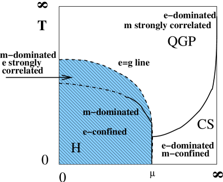
We, on the other hand, focus on the competition of EQPs and MQPs and divide the phase diagram differently, into (i) the “magnetically dominated” region at $T<T_{E=M}$ and (ii) “electrically dominated” one at $T>T_{E=M}$. In our opinion, the key aspect of the physics involved is the coupling strength of both interactions. So, a divider is some E-M equilibrium region at intermediate $T$-$\mu$. Since it does $not$ correspond to a singular line, one can define it in various ways: the most direct one is to use a condition that electric (e) and magnetic (g) couplings are equal

$$e^{2}/{\hbar c}=g^{2}/{\hbar c}=1/2$$ (1)

The last equality follows from the celebrated Dirac quantization condition [1]

$$\frac{eg}{\hbar c}=\frac{n}{2}$$ (2)

with $n$ being an integer, put to 1 from now on.

Besides equal couplings, the equilibrium region is also presumably characterized by comparable densities as well as masses of both electric and magnetic quasiparticles.

The “magnetic-dominated” low-$T$ (and low-$\mu$) region (i) can in turn be subdivided into the $confining$ part (i-a) in which electric field is confined into quantized flux tubes surrounded by the condensate of MQPs, forming t’Hooft-Mandelstamm “dual superconductor” [2], and a new “postconfinement” region (i-b) at $T_{c}<T<T_{E=M}$ in which EQPs are still strongly coupled (correlated) and still connected by the electric flux tubes. We believe this picture better corresponds to a situation in which string-related physics is by no means terminated at $T=T_{c}$: rather it is at its maximum there. Then if leaving this “magnetic-dominated” region and passing through the equilibrium region by increase of $T$ and/or $\mu$, we enter either the high-$T$ ”electric-dominated” QGP or a color-electric superconductor at high-$\mu$ replacing the dual superconductor (with diquark condensate taking place of monopole condensate).

A phase diagram explaining this viewpoint pictorially is shown in Fig.1.

The paper is structured as follows. We start with a mini-review of the subject, including RHIC phenomenology and lattice data relevant for this picture. Then we start discussing classical dynamics of electric and magnetic charges interacting with each other. We briefly summarize what is known about the two-body problems in section II, and proceed to (idealized) 3-body problem, namely a motion of a magnetically charged object in a field of a static electric dipole, and discuss flux tubes in classical plasmas. We then proceed to Molecular Dynamics (MD) simulations. The main parameters of the model are (i) the ratio of MQPs/EQPs concentration and (ii) the ratio of magnetic-to-electric coupling $g/e$. The main issues discussed are how the transport properties (in particular the $shear$ $viscosity$) of the plasma depend on them. More specifically, the issue is whether admixture of weaker-coupled MQPs increases or decreases it.

FIG. 1.: (color online) A schematic phase diagram on a (“compactified”) plane of temperature and baryonic chemical potential $T-\mu$. The (blue) shaded region shows “magnetically dominated” region $g<e$, which includes the e-confined hadronic phase as well as “postconfined” part of the QGP domain. Light region includes “electrically dominated” part of QGP and also color superconductivity (CS) region, which has e-charged diquark condensates and therefore obviously m-confined. The dashed line called “e=g  line” is the line of electric-magnetic equilibrium. The solid lines indicate true phase transitions, while the dash-dotted line is a deconfinement cross-over line.

A Strongly coupled Quark-Gluon plasma in heavy ion collisions

A realization [3, 4] that QGP at RHIC is not a weakly coupled gas but rather a strongly coupled liquid has led to a paradigm shift in the field. It was extensively debated at the “discovery” BNL workshop in 2004 [5] (at which the abbreviation sQGP was established) and multiple other meetings since.

Collective flows, related with explosive behavior of hot matter, were observed at RHIC and studied in detail: the conclusion is that they are reproduced by the ideal hydrodynamics remarkably well. Indeed, although these flows affect different secondaries differently, yet their spectra are in quantitative agreement with the data for all of them, from $\pi$ to $\Omega^{-}$. At non-zero impact parameter the original excited system is deformed in the transverse plane, creating the so called elliptic flow described by

$$v_{2}(s,p_{\,t},M_{i},y,b,A)=<cos(2\phi)>$$ (3)

where $\phi$ is the azimuthal angle and the others stand for the collision energy, transverse momentum, particle mass, rapidity, centrality and system size. Hydrodynamics explains all of those dependence, for about 99% of the particles.

Naturally, theorists want to understand the nature of this behavior by looking at other fields of physics which have prior experiences with liquid-like plasmas. One of them is related with the so called AdS/CFT correspondence between strongly coupled $\cal N$=4 supersymmetric Yang-Mills theory (a relative of QCD) to weakly coupled string theory in Anti-de-Sitter space (AdS) in classical SUGRA regime. We will not discuss it in this work: for a recent brief summary of the results and references see e.g. [6].

Zahed and one of us [4] argued that marginally bound states create resonances which can strongly enhance transport cross section. Similar phenomenon does happen for ultracold trapped atoms, due to Feshbach-type resonances at which the binary scattering length $a\rightarrow\infty$, which was indeed shown to lead to a near-perfect liquid. van Hees, Greco and Rapp[7] studied $\bar{q}c$ resonances, and found enhancement of charm stopping.

Combining lattice data on quasiparticle masses and interparticle potentials, one finds a lot of quark and gluon bound states [8, 9] which contribute to thermodynamical quantities and help explain the “pressure puzzle” [8], an apparent contradiction between heavy quasiparticles near $T_{c}$ and rather large pressure. The magnetic sector discussed in this paper provides another contribution, that of MQPs (monopoles and dyons), which will help to resolve the pressure puzzle.

A very interesting issue is related with counting of the bound states of all quasiparticles. Here the central notion is that of curves of marginal stability (CMS), which are not thermodynamic singularities but lines indicating a significant change of physics where a switch from one language to another (like E$\rightleftharpoons$M ) is appropriate or even mandatory.

Let us mention one example related with quite interesting “metamorphosis” discussed in literature, in the context of $\cal N$=2 SUSY theories. The CMS in question is related with the following reaction

$$gluon\leftrightarrow monopole+dyon$$ (4)

in which the r.h.s. system is magnetically bound pair (obviously with zero total magnetic charge). The curve itself is defined by the equality of thresholds,

$$M(gluon)=M(dyon)+M(monopole)$$ (5)

As discussed in details by Ritz et al [10] , inside the region surrounded by CMS (in which the state in the r.h.s. is $lighter$ than the gluon) even a notion of a gluon as a separate state does not exist, and using the “magnetic language” (r.h.s.) for its description becomes mandatory.

B Classical Molecular Dynamics for non-Abelian plasmas

Another direction, pioneered by Gelman, Zahed and one of us [11], is to use experience of classical strongly coupled electromagnetic plasma. Their model for the description of strongly interacting quark and gluon quasiparticles as a classical and non-relativistic Non-Abelian Coulomb gas. The sign and strength of the inter-particle interactions are fixed by the scalar product of their classical color vectors subject to Wong’s equations. The EoM for the phase space coordinates follow from the usual Poisson brackets:

$$\{x_{\alpha\,i}^{m},p_{\beta\,j}^{n}\}=\delta^{mn}\delta_{\alpha\beta}\delta_{ij}\,\,\,\,\{Q_{\alpha\,i}^{a},Q_{\beta\,j}^{b}\}=f^{abc}\,Q_{\alpha\,i}^{c}$$ (6)

For the color coordinates they are classical analogue of the SU(N_c) color commutators, with $f^{abc}$ the structure constants of the color group. The classical color vectors are all adjoint vectors with $a=1...(N_{c}^{2}-1)$. For the non-Abelian group SU(2) those are 3d vectors on a unit sphere, for SU(3) there are 8 dimensions minus 2 Casimirs=6 d.o.f..

This cQGP model was studied using Molecular Dynamics (MD), the equations of motion were solved numerically for $n\sim 100$ particles. It also displays a number of phases as the Coulomb coupling is increased ranging from a gas, to a liquid, to a crystal with anti-ferromagnetic-like color ordering. There is no place for details here, let us only mention that important transport properties like diffusion and viscosity vs coupling. note how different and nontrivial they are. When extrapolated to the sQGP suggest that the phase is liquid-like, with a diffusion constant $D\approx 0.1/T$ and a bulk viscosity to entropy density ratio $\eta/s\approx 1/3$. The second paper of the same group[11] discussed the energy and the screening at $\Gamma>1$, finding large deviations from the Debye theory.

The first study combining classical MD with quantum treatment of the color degrees of freedom has been attempted by the Budapest group [12].

C Electric-magnetic dualities in supersymmetric theories

Progress in supersymmetryc (SUSY) Quantum Field Theories was originally stimulated by a desire to get rid of perturbative divergencies and solve the so called hierarchy problems. However in the last 2 decades it went much further than just guesses of possible dynamics at superhigh energies. A fascinating array of nonperturbative phenomena have been discovered in this context, making them into an excellent theoretical laboratory. However we think that their relevance to QCD-like theories are neither understood not explored in a sufficient depth yet.

Studies of instantons in these theories have resulted in exact beta functions [13] and other tools, which have allowed Seiberg to get quite complete picture of the phase structure of ${\cal N}\,\,$=1 SUSY gauge theories [14].

This was enhanced in the context of ${\cal N}\,\,$=2 SUSY gauge theories by Seiberg and Witten [15], who were able to show how physical content of the theory changes as a function of Higgs VeVs (in a “moduli space” of possible vacua). Singularities in moduli space were identified with the phase transitions, in which one of the MQPs gets massless. Seiberg and Witten have found a fascinating set of $dualities$, explaining where and how a transition from one language to another (e.g. from “electric” to “magnetic” to “dyonic” ones) can explain what is happening at the corresponding part of the moduli space, in the simplest and most natural way.

One lesson from those works, which is most important for us, is what happens with the strength of electric $e$ and magnetic coupling $g$ near the phase transition. As e.g. monopoles gets light and even massless at some point, the “Landau zero charge” in the IR is enforced by the $U(1)$ beta function of the magnetic QEDs, making them weakly coupled in IR, $g<<1$. The Dirac quantization (2) therefore demands that the electric coupling must get large $e>>1$, enforcing the “strongly coupled” electric sector in this region.

Since two pillars of this argument – $U(1)$ beta function and Dirac quantization – do not depend on supersymmetry or any other details of the SW theory, we therefore now propose it to be a generic phenomenon. We thus conjecture it to be also true near the QCD deconfinement transition $T\approx T_{c}$, explaining why phenomenologically we see a strong coupling regime there.

The high-$T$ limit, on the other hand, is similar to large-VEV domain of moduli space: here the $SU(N)$ asymptotic freedom in UV plus screening makes the electric charge small. Thus here MQPs are heavy and strongly coupled.

D Lessons from lattice gauge theory

Static potentials. One of the principal reasons we proposed to change the traditional viewpoint of putting confinement at the center, can be explained using lattice data on the $T-$dependence of the so called “static potentials”. The traditional reasoning points to the free energy $F(r,T)$ associated with static quark pair separated by a distance $r$, and defines the deconfinement as the disappearance of a (linearly) growing “string” term in it, so that at $T>T_{c}$ there is a finite limit of the free energy at large distances, $F(\infty,T)$. This phenomenon has often been referred to as a “melting of the confining string” at $T_{c}$.

FIG. 2.: The energy (a) and entropy (b) (as $TS_{\infty}(T)$) derived from the free energy of two static quarks separated by large distance, in $2$-flavor QCD according to [17].

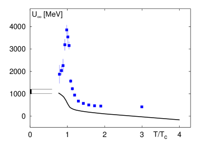
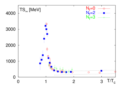
However, as explained by Polyakov nearly 3 decades ago [16], the string actually should not disappear at $T_{c}$: at this point its energy gets instead $compensated$ by the entropy term so that the $free$ energy $F=U-TS$ vanishes. As detailed lattice studies revealed, in fact the energy and entropy associated with a static quark pair are strongly peaked exactly at $T\approx T_{c}$, see Fig.2. The potential energy is really huge there, reaching about 4 GeV(!), while the associated entropy reaches equally impressive value of about 20. Nothing like that can be explained on the basis of Debye-screened weakly coupled gas of EQPs – the usual picture of QGP until few years ago. We think that the explanation of such large energy and huge number $\sim exp(20)$ of occupied states can only be obtained if several correlated quasiparticles are bound to heavy charges, presumably in the form of gluonic chains or “polymers” [9] conducting the electric flux from one charge to another.

Therefore, the “deconfinement” seen in disappearing linear term in free energy is actually restricted to static (or adiabatically slowly moving) charges, while for finite-frequency motion of light or even heavy (charmed) quarks one still should find mesonic bound states even in the deconfined phase [8]. Lattice studied of light quark and charmonium states [18] found that they indeed persist till $T\approx 2T_{c}$: this conclusion was dramatically confirmed by experimental discovery that $J/\psi$ suppression at RHIC is smaller than expected and is consistent with a new view, that $J/\psi$ is $not$ melting at RHIC (where $T<2T_{c}$).

One set of well-known lattice studies have tried to answer the following questions: Is a “dual superconductor” picture consistent with what is observed on the lattice? In particular, is the shape and field distribution inside the confining strings in agreement with that in the Abrikosov flux tube of a superconductor (Abelian Higgs model)? As one can read e.g. in [19], the answer seems to be a definite yes. Can one define in some way monopoles and their paths, and are those (in average) consistent with dual Maxwell equations? As one can read in e.g. [20], the answer seems to be also yes.

Unfortunately, those studies (as reviewed in [21]) were mostly concentrated in the vacuum $T=0$, while we are interested by the deconfined plasma $T>T_{c}$. Is there any general reason to think that MQPs play an important role here as well? The most important argument is the persistence of static magnetic screening at all $T$, up to infinitely high $T$.

Screening. Although static magnetic screening was shown to be absent in perturbative diagrams [22], it has been conjectured by Polyakov [16] to appear nonperturbatively at the “magnetic scale” which at high $T$ is

$$\Lambda_{M}=e^{2}T$$ (7)

The magnetic screening mass and monopole density should thus be

$$M_{M}=C_{M}\Lambda_{M},\hskip 28.45274ptn_{M}=C_{n}\Lambda_{M}^{3}$$ (8)

with some numerical constants $C_{M},C_{n}$.

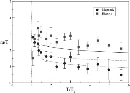
To illustrate current lattice results, we show the $T$-dependence of the electric and magnetic screening masses calculated by Nakamura et al [23], see Fig.3. Note that electric mass is larger than magnetic one at high $T$, but vanishes at $T_{c}$ (because here electric objects gets too heavy and effectively disappear). The magnetic screening mass however grows toward $T_{c}$, which is consistent with its scaling estimate

$$M_{M}^{2}\sim(e^{2}T)^{2}$$ (9)

(Another estimate of the magnetic screening can be done in the dual language as

$$M_{M}^{2}\sim g^{2}n_{M}/T\sim g^{2}(e^{2}T)^{3}/T$$ (10)

which is a perturbative (small magnetic coupling $g$) loop: note that it agrees with the former one due to Dirac condition $e\sim 1/g$.)

If one uses screening masses to get an idea about density of electric and magnetic objects, one finds that the point at which electric and magnetic masses are equal should be close to the E-M equilibrium point we emphasized above. This argument places the equilibrium temperature somewhere in the region of

$$T_{E=M}\approx(1.2-1.5)T_{c}=250-300\,MeV$$ (11)

.

FIG. 3.: Temperature dependence of electric and magnetic screening masses according to Nakamura et al [23]. The dotted line is fitted by the assumption, $m_{g}\sim g^{2}T$. For the electric mass, the dashed and solid lines represent LOP and HTL resummation results, respectively.

High-T monopoles. The total pressure related to magnetic (3d) sector of the theory and especially the spatial string tension are other observable related to MQPs above $T_{c}$: for a short recent summary see [24]. Two important points made by Korthals-Altes are: (i) MQPs must be in the $adjoint$ color representation, to explain data on k-strings and magnetic pressure; (ii) there seems to be a nontrivial small “diluteness” parameter of the MQPs ensemble

$$\delta={\sigma_{1}\over M_{M}^{2}}\approx{(N-1)n_{M}\over M_{M}^{3}}\approx{1\over 20}$$ (12)

The fact that screening takes place at distances $smaller$ than the average inter-MQP ones is a clear indication that screening is not a Debye-type weak coupling one, but rather the opposite $strongly$ coupled (correlated) screening.

Dyons. A very special sector of MQPs are particles with both charges. Because they produce parallel electric and magnetic fields, they have nonzero $(\vec{E}\vec{B})$ and thus the topological charge. In fact, as shown by Kraan et al [25], finite-$T$ instantons can be viewed as being made of $N_{c}$ self-dual dyons: for a very nice AdS/CFT “brane-based” construction leading to the same conclusion, see [26].

Topology is in turn associated with the Dirac zero eigenvalues for fermions, which can be located and counted on the lattice quite accurately. Furthermore, a “visualization” of dyons inside lattice gauge field configurations (using variable non-trivial holonomy) has been developed into a very sensitive tool [27], revealing multi-dyon configurations and their dynamics. One can verify that they make a rather dilute but highly correlated systems: in fact closed chains of up to 6 dyons of alternating charges have been seen. The self-dual dyon density and other properties, as well as their relation to instantons and confinement are summarized in recent paper [28]. It is enough to mention only that self-dual dyons, like instantons, are electrically screened [29, 30] and thus rapidly disappear into the QGP at $T>T_{c}$. Around $T_{c}$ their density can thus be related to the instanton density

$$n_{dyon}\sim N_{c}n_{instantons}/T\sim 3fm^{-3}$$ (13)

and the mass to the instanton action

$$M_{dyon}=T*S_{instanton}/N_{c}\sim(3-4)T$$ (14)

Both are of the order of the density (and the mass) of the electric (gluon and quark) quasiparticles at $1.5T_{c}$, confirming a suggested E-M equilibrium in this region.

E Higgs phenomenon in QGP?

In this subsection we would like to comment, in a brief form, on a number of questions which are invariably asked in connection with Higgs phenomenon and monopoles at $T>T_{c}$.

Naively, there is no simple and direct way to apply the lessons from supersymmetric theories such as $\cal N$=2 Seiberg-Witten theory to QCD-like setting. The former has scalar fields and flat “moduli space” of possible vacua, while the latter has neither scalars nor supersymmetry to keep the moduli space flat.

At finite $T$ the role of Higgs field is delegated to temporal component $A_{0}$ of the gauge field: and in fact in gluodynamics there is a spontaneous breaking of the $Z(N_{c})$ symmetry at $T>T_{c}$ because the corresponding effective action $S_{eff}(<A_{0}>)$ has $N_{c}$ discrete degenerate minima.

Furthermore, the corresponding effective action gets small near $T_{c}$ and large fluctuations in “Higgs VEV” $<A_{0}>$ are seen in lattice configurations; so one may think first about a generic case in which it is some (color matrix valued) constant in each configuration, to be averaged with appropriate weight $exp[-S_{eff}(<A_{0}>)]$ later. Thus one may think about an explicit adjoint Higgs breaking of the color group, parameterized by $N_{c}-1$ real VEVs (e.g. for $SU(3)$ $Tr<A_{0}\lambda^{a}>$with Gell-Mann diagonal matrices a=3,8). Such breaking makes all gluons massive, except the remaining unbroken $N_{c}-1$ U(1)’s which remain massless. These remaining U(1)’s are the Abelian gauge fields which define magnetic charges of the monopoles and their long-range interactions (and electric ones, in the case of dyons).

Finally, the last comment about one lesson from SUSY theories which we don’t think can be transferred into the QCD world: these are the enforced properties of monopoles (and many other topological objects like branes) which happen to be “BPS states” with their Coulomb interactions being exactly cancelled by massless scalar exchanges. As a result, such objects can often “levitate” in SUSY settings. In QCD we however do not see or need massless scalars, leaving the usual Coulomb and Lorentz forces dominant at large distances.

II Few-body problems with Magnetic charges

The simplest few-body system with magnetic charge is made of two particles: one has electric charge and the other has magnetic charge. In a more general sense we should consider them as two dyons, both with nonzero electric as well as magnetic charges. This problem has been very well studied for many years in both classical and quantum mechanics, and it has fascinated the physicists with many unusual features. See for example [31][32][33].

In such problems one has both electric and magnetic fields. We have the electric field from an E-charge (at space point $\vec{r}_{e}$) to be

$$\vec{E}(\vec{r})=e\frac{\vec{r}-\vec{r}_{e}}{|\vec{r}-\vec{r}_{e}|^{3}}$$ (15)

and magnetic field from a M-charge (at space point $\vec{r}_{g}$) to be

$$\vec{B}(\vec{r})=g\frac{\vec{r}-\vec{r}_{g}}{|\vec{r}-\vec{r}_{g}|^{3}}$$ (16)

The interaction between one moving dyon $(e_{1},g_{1})$ and the other $(e_{2},g_{2})$ is given by the Coulomb and $O(v/c)$ Lorentz forces

$$\vec{F}_{12}= (e_{2}\cdot e_{1}+g_{2}\cdot g_{1})\frac{\vec{r}}{r^{3}}$$ (18)

$$+(e_{2}\cdot g_{1}-g_{2}\cdot e_{1})\frac{\vec{v}_{2}}{c}\times\frac{\vec{r}}{r^{3}}+O(v^{2}/c^{2})$$

with $\vec{r}=\vec{r}_{2}-\vec{r}_{1}$. Here we have used the Gaussian units in which $\vec{E}$ and $\vec{B}$ have the same unit and so are the charges $e$ and $g$.

As early as in 1904, J. J. Thomson found the even two non-moving charges have a nonzero angular momentum $J$ carried by rotating electromagnetic field . Indeed, for an E-charge and a M-charge (separated by $\vec{r}$) as sources, it is

$$\vec{J}_{field}=\int d^{3}x\vec{x}\times\frac{\vec{E}\times\vec{B}}{4\pi c}=\frac{eg}{c}\hat{r}$$ (19)

This angular momentum depends only on the value of charges, independent on how far or close they may be. Its direction is radial, pointing from the E-charge to the M-charge.

FIG. 4.: The trajectory of a dyon in a field of static charge.

Even earlier, in 1896 Poincare observed that a dyon moves in a charge Coulomb field on the surface of a cone, as shown in Fig.4. Their relative motion (angular rotation and radial bouncing ) is always confined inside a cone simply because of the conservation of total angular momentum including the relative rotation and the field’s angular momentum (19) as well. When getting closer to each other the two particles are forced to rotating faster thus experiencing effective repelling which makes them bouncing radially. Another way to explain the conical motion is to notice that a magnetic charge is making Larmor circles around the electric field; it shrinks near the charge because the fields gets stronger there.

Quantum mechanics of such two-dyon system has been worked out in many details since 1970s, especially the many bound states are calculated, see [32, 33] for review.

A Static Electric Dipole and a Dynamical Monopole

A very interesting and important few-body problem is a magnetic monopole moving in the field of a static electric dipole. This is a starting point for studying a ”color”-electric dipole(quark-anti-quark) surrounded by a gas of weakly interacting monopoles which, as we argue, may be very much relevant for understanding confinement. Also as far as we know, this system seems never been studied before.

FIG. 5.: Trajectory of monopole motion in a static electric dipole field (with charges at $\pm 1\,\hat{z}$) as (left panel)projected on x-y plane and (right panel)projected on R-z plane ($R=\sqrt{x^{2}+y^{2}}$).

FIG. 6.: Trajectory of monopole motion in a static electric dipole field (with charges at $\pm 1\,\hat{z}$) as (left panel)projected on x-y plane and (right panel)projected on R-z plane ($R=\sqrt{x^{2}+y^{2}}$).

Considering quark-anti-quark pair surrounded by a gas of weakly interacting monopoles as the scenario for confining the flux tube just around $T_{c}$, one realize that to find possible bound states (namely, states with the monopole attached around the electric dipole permanently or at least for long time before ”decaying” away) of such a system is potentially a key to understand the source of large entropy associated with static quark-anti-quark as indicated by lattice. We will discuss this issue in both classical and quantum mechanics.

In classical mechanics, we have the EoM for the monopole (of mass $m$ and magnetic charge $g$) to be the following:

$$m\frac{d^{2}\vec{r}}{dt^{2}}=g\vec{E}_{d}\times\frac{d\vec{r}}{dt}$$ (20)

with $\vec{E}_{d}$ the electrostatic field from the dipole with $\pm e$ charges sitting at $\pm a$ on $z$ axis:

$$\vec{E}_{d}=e\,{\bigg{[}}\frac{\vec{r}-a\hat{z}}{|\vec{r}-a\hat{z}|^{3}}-\frac{\vec{r}+a\hat{z}}{|\vec{r}+a\hat{z}|^{3}}{\bigg{]}}$$ (21)

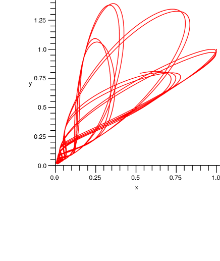
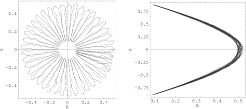
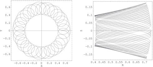
It will be much convenient to work in the cylinder coordinate $(\rho,\phi,z)$. By running this EoM numerically with various initial conditions, we can directly obtain real time trajectories of the monopole.

FIG. 7.: Trajectory of monopole motion in a static electric dipole field (with charges at $\pm 1\,\hat{z}$) as (left panel)projected on x-y plane and (right panel)projected on R-z plane ($R=\sqrt{x^{2}+y^{2}}$).

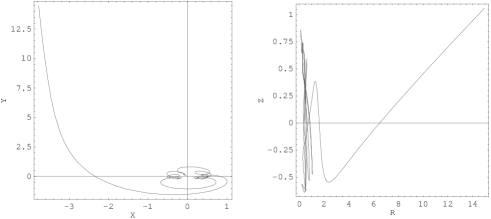
A lot of very complicated and very different motions have been found, sensitively depending on the initial conditions. Roughly one may divide these trajectories into two categories: ”trapping” cases (see Fig.5 and Fig.6) and ”escaping” cases (see Fig.7). By ”trapping” cases we mean the monopole starts with $|\vec{r}|\sim a$ and after a relatively long time it still remains within distance $\sim a$ from the dipole, while in ”escaping” cases the monopole begins moving further and further away from the dipole after a somewhat short time. Due to limited space we show below only few pictures for both cases. Let’s just emphasize one particular feature as clearly revealed in Fig.5: the monopole is bouncing back and forth between the two electric charges, because of the effective repulsion when it is getting close to the charges (as has been explained in the charge-monopole motion). We have found many such cases which look like two standing charges playing E-M ”ping-pong” with the monopole. So there are many classical bound states for such system, and in principle one can scan through the phase space of monopole’s initial position and momentum to estimate the ”trapping” states’ phase space volume.

This phenomenon as shown here is dual to the famous “magnetic bottle”, a device invented for containment of hot electromagnetic plasmas, provided magnetic coils at its ends are substituting the electric dipole and a moving monopole replaced by the electric charge.

Now let’s turn to the quantum mechanics of such system. One can write down the following Hamiltonian for the monopole:

$$\hat{\cal H}=\frac{(\vec{p}+g{\vec{A}_{e}})^{2}}{2m}$$ (22)

Here $\vec{A}_{e}$ is the electric vector potential of the dipole electric field, which can be thought of as a dual to the normal magnetic vector potential of a magnetic dipole made of monopole-anti-monopole. By symmetry argument we can require the vector potential as $\vec{A}_{e}=A^{\phi}_{e}(\rho,z)\hat{\phi}$ and the monopole wavefunction as $\Psi=\psi(\rho,z)e^{if\phi}$ with $f$ the z-angular-momentum quantum number. Then the stationary Schroedinger equation is simplified to be

$$[\frac{\vec{p}_{\rho}^{\,\,2}+\vec{p}_{z}^{\,\,2}}{2m}+V_{eff}]\psi=E\psi$$ (23)

$$V_{eff}=\frac{\hbar^{2}}{2m}[\frac{1}{\rho/a}(\frac{ge}{\hbar}\frac{\rho A_{e}^{\phi}}{e}+f)]^{2}$$ (24)

To go further one has to specify a gauge (which is equivalent to choosing some particular dual Dirac strings for the charges) so as to explicitly write down $A_{e}^{\phi}$. We use the gauge which corresponds to the situation with one Dirac string going from the positive charge along positive $\hat{z}$ axis to $+\infty$ and the other going from the negative charge along negative $\hat{z}$ axis to $-\infty$. This gives us:

$$A_{e}^{\phi}=-\frac{e}{\rho}[2+\frac{z-a}{\sqrt{\rho^{2}+(z-a)^{2}}}-\frac{z+a}{\sqrt{\rho^{2}+(z+a)^{2}}}]$$ (25)

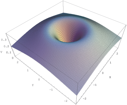
To give an idea of the effective potential we show Fig.8 where $V_{eff}(\rho,z,f)=V_{eff}(\sqrt{x^{2}+y^{2}},z,f)$ is plotted for the x-y plane with $z=0$ and $f=0$. From the plot we can see that there must also be quantum states with the monopole bounded within the potential well around the dipole for a long time before eventually decaying away. Namely one can find states with $E=\hbar\omega+i\Gamma$ with $\Gamma<<\hbar\omega$ and count how many there are. This issue will be separately addressed in details elsewhere.

FIG. 8.: (color online) Quantum mechanical effective potential for a monopole in a static electric dipole field. See text for details.

B Flux tubes in a classical gas

The problem discussed in the previous subsection has of course not only “trapped” monopole states emphasized above, but also a lot of scattering states for monopoles with positive energy. In a simple classical setting it is quite clear that in an ensemble (gas) of monopoles, particles would scatter off the effective positive potential depicted in Fig.8 and provide effective pressure on it. The net result should be nothing but stabilization of the $electric$ flux tubes in a gas of monopoles, at a size equilibrating gas pressure with the field stress tensor.

The situation dual to the problem discussed is $magnetic$ flux tubes in a gas of electric charges. Since this does not need magnetic charges, it takes place in electrodynamic plasmas. As a well known example, stabilized magnetic flux tubes are found in the solar plasma: there they extend for millions of kilometers and are seen in a modern telescope as a substructure of “solar black spots”.

Although we would discuss classical flux tubes in a separate paper, we would like to point out now their role in our general picture. We believe those occur at two extremes: (i) at $T$ just above $T_{c}$, as classical electric flux tubes are expelled by dominant MQPs, and (ii) at very high $T$ when there are magnetic flux tubes expelled by dominant EQPs. In the former case electric flux tubes are a natural continuation of $quantum$ electric flux tubes which are created by Bose-condensed MQPs in the confining phase at $T<T_{c}$. What we would like to point out here is that MQPs expel the electric field lines out of the volume they occupy irrespective whether they are Bose-condensed or not.

III Molecular dynamics without periodic boxes

Molecular dynamics (MD) provides a straightforward way to study the various dynamical properties of a classical many-body system. The system we are interested in is a plasma containing both electric and magnetic (and both positive and negative) charges. So in the normal convention used by plasma physics community, this is a four-component-plasma(FCP). We however would rather name it as 2E-2M-plasma to explicitly show its content. More widely speaking we may even include one more type of particles, namely dyons with both electric and magnetic charges for individual particles, making a 2E-2M-4D-plasma. In this paper we will report our results for 2E-2M-plasma with three different contents: pure electric (which reduces to normal TCP) plasma, plasma with about one quarter of particles as magnetic charges, and plasma with about half of particles as magnetic charges, labelled throughout this paper as M00, M25, M50 respectively. Comparison among them is expected to give indications about the role of magnetic charges, especially in the transport properties. The microscopic dynamics is classical EM, given by Newton’s second law together with electric Coulomb force (between two E-charges), magnetic Coulomb force (between two M-charges) and $O(v)$ Lorentz force (between one E-charge and one M-charge).

The routine MD method (as used in GSZ and most MD study of usual plasma) is to put desired number of particles in a cubic box and then include as many periodical image boxes (in all three directions) as allowed by computing capacity. The summation over images is very much time consuming especially for cases with Coulomb type long range forces. Also energy conservation is not very well preserved after long-time run because of the ”kick” on particles leaving one truncation boundary and entering periodically on the opposite boundary which will gradually heat up the system.

Here it should be emphasized that we have used an alternative approach without any periodic boxes. What we have done is to simply give all particles certain initial conditions and then let them go. It turns out there are two different regimes which we deal with separately: 1) ”plasma in cup” at medium/weak coupling regime, in which case we place a sharply rising large radial potential barrier at certain radial distance to hold the particles inside this ”cup”; 2) ”self-holding drop” at very strongly coupled regime, which means the particles don’t fall apart into small pieces but behave like a little raindrop and so there is no need for a ”cup”. In this way we are able to perform MD easily with thousand particles and can conserve energy for less than percent even after really long-time run. We will give more technical details about our simulations in the second subsection while present basic formulae, units and physical parameters in the first subsection .

A Formulae,units and physical parameters

For our 2E-2M-plasma, each particle has either electric charge or magnetic charge. The E-charges are assigned as $e_{i}e$ with $e_{i}$ randomly and equally given $\pm 1$ ($e_{i}=0$ for M-charges) and the M-charges are assigned as $g_{i}g$ with $g_{i}$ randomly and equally given $\pm 1$ ($g_{i}=0$ for E-charges) too. For a pair of particles their mutual force involves three combinations of their charges: $e_{ij}=e_{i}\cdot e_{j}$, $g_{ij}=g_{i}\cdot g_{j}$, and an important new one $\kappa_{ij}=e_{i}\cdot g_{j}-g_{i}\cdot e_{j}$. In present study we use the same mass $m$ for both types of charges.

The equation of motion for the $i$th component particle is given by:

$$m\frac{d^{2}\vec{r}_{i}}{dt^{2}}=\sum_{j\neq i}{\bigg{[}}\frac{C}{r_{ij}^{K+1}}\hat{r}_{ji} +\frac{e^{2}\,e_{ij}}{r_{ij}^{2}}\hat{r}_{ji}$$ (27)

$$+\frac{g^{2}\,g_{ij}}{r_{ij}^{2}}\hat{r}_{ji}+\frac{ge\,\kappa_{ij}}{r_{ij}^{2}}\frac{d\vec{r}_{i}}{c\,dt}\times\hat{r}_{ji}{\bigg{]}}$$

where $\vec{r}_{ji}=\vec{r}_{i}-\vec{r}_{j}$. The first term on RHS is the well-known necessary repulsive core without which all classical plasma will collapse sooner or later since no quantum effect arises at small distance to prevent positive charges falling onto negative partners. We choose $K=9$ in our MD, which is the same as some previous work[11][34]. There is no particular meaning for $K=9$ except that we want a large value of $n$ which leads to relatively small correction ($\sim 1/K$) to potential energy between $+e$ and $-e$ at and beyond the equilibrium distance.

To set the units in our numerical study, we use the following scaling for length and time (the unit of mass is naturally set by particle mass $m$)

$$\vec{\tilde{r}}=\vec{r}/r_{0}\qquad with\qquad r_{0}=(C/e^{2})^{\frac{1}{K-1}}$$ (28)

$$\tilde{t}=t/\tau\qquad with\qquad\tau=(mr_{0}^{3}/e^{2})^{\frac{1}{2}}$$ (29)

which leads to the dimensionless equation of motion

$$\frac{d^{2}\vec{\tilde{r}}_{i}}{d{\tilde{t}}^{2}}=\sum_{j\neq i}{\bigg{[}} \frac{1}{\tilde{r}_{ij}^{n+1}}\hat{r}_{ji}+\frac{e_{ij}}{\tilde{r}_{ij}^{2}}\hat{r}_{ji}$$ (31)

$$+(\frac{g}{e})^{2}\frac{g_{ij}}{\tilde{r}_{ij}^{2}}\hat{r}_{ji}+(\frac{g}{e}\frac{r_{0}/\tau}{c})\frac{\kappa_{ij}}{\tilde{r}_{ij}^{2}}\frac{d\vec{\tilde{r}}_{i}}{d\tilde{t}}\times\hat{r}_{ji}{\bigg{]}}$$

With these setting, we have for example: Length = # $\times r_{0}$, Time = # $\times\tau$, Frequency = # $\times\frac{1}{\tau}$, Velocity = # $\times\frac{r_{0}}{\tau}$, Energy = # $\times\frac{e^{2}}{r_{0}}$, etc. All numbers obtained from numerics are subjected to association with proper dimensional factors in our units.

Now we still have two dimensionless physical parameters which controls in the above the magnetic-related coupling strength:
1. $\tilde{g}=\frac{g}{e}$ : this parameter characterizes the relative coupling strength of magnetic to electric sector. In principle there is no limitation for it from classical physics. Since we want to focus on the parametric regime which may be relevant to sQGP problem near $T_{c}$ (where electric sector gets strongly coupled while magnetic sector gets weak), the parameter $\tilde{g}$ is expected to be small, so we will use $\tilde{g}=0.1$ in the MD calculation. Naively suppose one has a quantum problem with same $\tilde{g}=g/e$, then by combination with the minimum Dirac condition $\frac{eg}{\hbar c}=\frac{e^{2}}{\hbar c}\tilde{g}=\frac{1}{2}$, one gets $\alpha=\frac{e^{2}}{\hbar c}=1/(2\tilde{g})\sim 5$ which is indeed very strongly coupled.
2. $\beta=\frac{r_{0}/\tau}{c}=\sqrt{\frac{e^{2}/r_{0}}{mc^{2}}}$ : this parameter tells us how relativistic the particles’ motion will typically be. The importance of this parameter lies in that it controls the strength of Lorentz force ($\beta\cdot\tilde{g}$) between E-M charges. An important observation here is that compared to the Lorentz coupling of a pure electric plasma (which is $\beta^{2}$ from electric current-current) our Lorentz force has only the first power of the small parameter $\beta$ and is thus enhanced because of the existence of magnetic charges. Since we are doing non-relativistic molecular dynamics, a small value of $\beta$ should be chosen. In the sQGP the typical speed is estimated to be about $1/3$ of $c$, in present calculation we however will choose $\beta=0.1$ which on one hand is not far from $1/3$ and yet on the other hand limits the relativistic corrections to be not more than few percent.

One more physical parameter we should mention here is the so called plasma parameter $\Gamma$ defined as the ratio of average potential kinetic energy (neglecting the sign)

$$\Gamma={\bigg{|}}\frac{<U>}{<E_{k}>}{\bigg{|}}={\bigg{|}}\frac{<U/N>}{3k_{B}T/2}{\bigg{|}}$$ (32)

This definition looks a little different from others[11][34] where usual MD study with periodic boxes defines $\Gamma=\frac{e^{2}/a}{k_{B}T}$ with $a=(3/4\pi n)^{1/3}$. They use this conveniently because in their approach the density is fixed as desired, while in our case there is no boxes any more and we use the direct ratio which is essentially meaning the same thing. The difference and relation between the two $\Gamma$ values will be further discussed in section V D.

The plasma parameter $\Gamma$ is important in that:
1. it distinguishes strongly coupled plasma $\Gamma>>1$ and weakly coupled plasma $\Gamma<<1$;
2. it roughly distinguishes a gas phase $\Gamma<1$, a liquid phase $\Gamma\sim 10$ and a solid (or solid-like) phase $\Gamma>100$ ;
3. different types of plasma with the same value of $\Gamma$ could be compared in order to reveal the dependence of macroscopic properties on plasma contents and microscopic dynamics, and so we will measure properties as a function of $\Gamma$.

B Details of MD simulations

In our MD simulations, 1000 particles are initially placed on the sites of a $10\times 10\times 10$ cubic lattice with lattice spacing $a=1.2r_{0}$ . They are given electric charges $\pm 1$ in an alternating way in all 3 directions. Then for the M25 (M50) plasma, we randomly pick out 25% (50%) of the particles and re-assign them magnetic charges instead of electric charges. Then all the particles are randomly given initial velocity (for each of the three component) $v^{i}_{1,2,3}(t=0)=V*(RANDOM\#)$ ($RANDOM\#$ is between [0,1]) under condition that the total velocity of the whole system is zero. For each type of plasma, changing the value of $V$ can eventually lead to different equilibrated system after certain time. Roughly the larger $V$ is, the smaller (lower) the plasma parameter $\Gamma$ (temperature $T$) will be. The total running time is $2000\Delta t$ with $\Delta t=0.1\tau$ (which is actually our output time step). In general it takes $t_{therm}\sim 20-30\tau$ to equilibrate the system and we start measurements at $t=50\tau$. The iteration step and accuracy in EoM subroutine is so chosen that the energy could be conserved to less than few percent at the end of run. As mentioned before, we have two different regimes which we will discuss the details separately in the following.

1 Plasma in cup

Numerically we found that for about $\Gamma<25$, the little drop we created couldn’t hold itself and after some running time it will break into a few much smaller pieces, which means the surface tension is not large enough to maintain the original ”big” drop. To confine the particles in a finite volume and make them mix up sufficiently, we put a radial potential barrier at some cut-distance $R_{cut}$ to make a container holding such plasma:

$$V=[B*(r-R_{cut})]^{L}*\theta(r-R_{cut})$$ (33)

By choosing $B=5$ and $L=11$ we make the edge of our ”cup” a really steep one, thus keeping as many particles inside the ”cup” as possible at all time because only very energetic particles are able to climb up the edge a little and will soon be reflected back. In our simulations we have used $R_{cut}=11r_{0}$. In real time of course the number of particles confined within the $R_{cut}$ is always fluctuating, so are other macroscopic quantities like energy etc. So this system is like a grand-canonical ensemble. For this plasma in cup, all the measurements are made for particles inside the cup only (namely with $r\leq R_{cut}$).

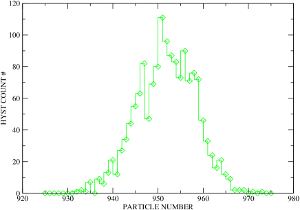
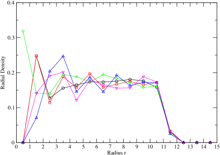
By looking at the histogram of total number of particles at different time points in Fig.9, one see that the system has very good distribution with well-defined average $N\sim 950$ and $\sqrt{N}\sim 30$ fluctuation width. Another important check is to see if the system is really homogeneous. In Fig.10 the radial local density $n(r)$ at five different time points (from early to very late time) are shown, from which it is clear that the density distribution is homogeneous and stable enough. The large fluctuation at very small r is understandable because one has much less particle numbers $n4\pi r^{2}$ for small r. One can also see that near our cutting edge ($R_{cut}=11$) the particle density quickly drops down as we want. These observations are true in all of our runs, and the number density of our cupped plasma at different $\Gamma$ is controlled all at $n\approx 0.17$ with negligible variation. These have shown that our simulations for cupped plasma is reliable.

FIG. 9.: (color online) Histogram of total number of particles inside $R_{cut}$ at 1500 different time points. This is an example from M25 plasma at $\Gamma=0.99$.

FIG. 10.: (color online) Radial density of particles as a function of radius $r$. The five curves are taken from different time points. This is an example from M25 plasma at $\Gamma=0.99$.

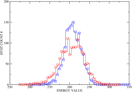
It is also important to check the fluctuation in energy. In Fig.11 we show a typical histogram of fluctuation in kinetic and potential energy at all time points. Clearly both distributions make complete sense and so are other macroscopic variables which we skip because of limited space. Again these justify our ”plasma-in-cup” approach.

FIG. 11.: (color online) Histogram of total kinetic(blue square) and potential(red circle)energy inside $R_{cut}$ at 1500 different time points. This is an example from M25 plasma at $\Gamma=0.99$.

The results to be reported in Section IV. and V. are all obtained with this method, which cover the $\Gamma$ value about $0.3-14$. We want to focus on this region because it is most relevant to the sQGP.

2 Self-holding drop

For about $\Gamma>25$ we have found our little drop can, amazingly, hold itself despite the possible expansion and shrinking with considerable amplitude. By mapping the particles’ coordinates at the end of run we found the particles more or less staying around their original positions. This very strongly coupled system behaves more like a crystal, especially for $\Gamma\to 100$. In this regime, we have found very good collective modes which are shown to manifest themselves in the dynamical correlation functions in a profound way. These results will be reported in section VI. It should be pointed out that the self-holding region is reached only for pure electric plasma (our M00 plasma). For our M25/M50 plasma, with present method the largest $\Gamma$ that can be achieved (after ”cooling” and equilibrating scheme) and maintained in a stable way is up to $\sim 25$. The ”cooling” method, namely turning on a braking force proportional to particle velocity for some time and then turning it off, can bring the M25/M50 system down to some instant $\Gamma\sim 1000$ but then the system kinetic energy slowly but steadily keeps increasing with potential energy getting more negative, the overall effect of which eventually increases $\Gamma$ back down to few tens. It seems indicating the mixture plasma refuses to become solidified even at classical level because of Lorentz type force (different from permanent liquid Helium which is due to quantum effect). We will leave this issue for future investigation.

IV Equation of state

Before showing the data, we once again emphasize that the goal is to compare three types of plasma (M00, M25, and M50) with different E-charges and M-charge concentration, and all the comparison will be made by plotting certain macroscopic properties as a function of plasma parameter $\Gamma$.

FIG. 12.: Temperature $T$ calculated at different plasma parameter $\Gamma$ in log-log plot for M00(triangle), M25(square), and M50(diamond) plasma respectively, with the three lines from linear fitting (see text).

The first quantity we want to look at is the temperature dependence on $\Gamma$ which is sort of equation of state for plasma. In Fig.12 the EoS for M00, M25, and M50 are compared in log-log plots. Data for all three show a linear relation with similar slopes but different intercepts. By simple linear fitting we get the following parameterized EoS for them:

$$M00\quad:\quad T=0.257\,/\,\Gamma^{\,0.827}$$ (34)

$$M25\quad:\quad T=0.191\,/\,\Gamma^{\,0.806}$$ (35)

$$M50\quad:\quad T=0.125\,/\,\Gamma^{\,0.759}$$ (36)

So already from the EoS we’ve seen considerable difference among the three plasma. Since EoS is important for dynamical processes, we proceed to study correlation functions and transport coefficients in next section, expecting to see more differences.

V Correlation functions and transport coefficients

Study of transport coefficients is very important in order to understand the experimental discoveries about sQGP, such as the very low viscosity and the diffusion of heavy quarks. In this section the transport coefficients of our three different plasma will be calculated and compared in order to see the influence of magnetic charges on the transport properties. To do that, we will first measure certain correlation functions and then relate them to the corresponding transport coefficients through the Kubo-type formulae, as is usually done in MD works.

A Velocity autocorrelation and diffusion constant

The first correlation function we will study is the velocity autocorrelation which is defined as:

$$D(\tau)=\frac{1}{3N}<\sum_{i=1}^{N}\vec{v}_{i}(\tau)\cdot\vec{v}_{i}(0)>$$ (37)

Here $\tau$ is the correlation time, $\vec{v}_{i}$ denotes the velocity of the $i$th particles and the sum is over all particles. The average is over thermal ensemble which is done in numerical program by average over all time points (with the number typically of order $\sim 1000$).

FIG. 13.: (color online) Velocity autocorrelation functions $D(\tau)$ for (from top down at zero time) M00(black curve), M25(green curve) and M50(red curve) plasma, taken at $\Gamma=1.01,0.99,1.00$ respectively.

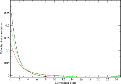
In Fig.13 we show typical curves for velocity autocorrelation function in M00, M25, and M50 plasma respectively. A fast damping behavior at small correlation time is observed, followed by small fluctuation from random noise at longer correlation time.

The corresponding transport coefficient, namely diffusion constant, is calculated by the following Kubo formula

$$D=\int_{0}^{\infty}D(\tau)\,d\tau$$ (38)

FIG. 14.: Diffusion constant $D$ calculated at different plasma parameter $\Gamma$ in log-log plot for M00(triangle), M25(square), and M50(diamond) plasma respectively, with the three lines from linear fitting (see text).

In Fig.14 we plot $LogD$ as a function of $Log\Gamma$ for M00,M25 and M50 plasma. Approximate linear relation is seen for all three, but with visible difference in slopes and intercepts. A linear fit gives the following approximate functions $D(\Gamma)$:

$$M00\quad:\quad D=0.396\,/\,\Gamma^{\,0.752}$$ (39)

$$M25\quad:\quad D=0.342\,/\,\Gamma^{\,0.707}$$ (40)

$$M50\quad:\quad D=0.273\,/\,\Gamma^{\,0.626}$$ (41)

At small $\Gamma<1$ there are considerable differences of the three lines. In the physically interesting region $\Gamma\sim 1-10$ the three plasma have visible but not too much difference in diffusion constants. The three lines will cross at about $\Gamma\sim 10$ and after that deviation from each other again grows quickly. The important feature common to all three types of plasma as well as to cQGP model in [11] is the power-law dropping of diffusion constant with increasing coupling strength. We see the diffusion constant can become few orders of magnitude smaller when one changes from weakly coupled gasous regime into strongly coupled liquid regime. This qualitative scaling in coupling is also found from AdS/CFT calculation by Casalderrey-Solana and Teaney in [35].

Interestingly if one combines (39) and (34), the dependence of $D$ on $T$ is then obtained:

$$M00\quad:\quad D=1.36\,T^{\,0.91}$$ (44)

$$M25\quad:\quad D=1.46\,T^{\,0.88}$$

$$M50\quad:\quad D=1.52\,T^{\,0.82}$$

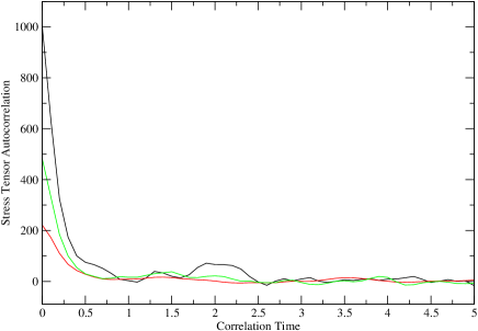
B Stress tensor autocorrelation and shear viscosity

It is of particular interest to study the shear viscosity of our three plasma, as the low viscosity is one of the most important discoveries for sQGP from RHIC experiments. For this purpose, one can measure the autocorrelation of the off-diagonal elements of stress tensor, namely

$$\eta(\tau)=\frac{1}{3VT}<\sum_{l<k}^{1,2,3}{\cal T}_{lk}(\tau){\cal T}_{lk}(0)>$$ (45)

with the stress tensor off-diagonal elements

$${\cal T}_{lk} = \sum_{i=1}^{N}m(\vec{v}_{i})_{l}(\vec{v}_{i})_{k}+\frac{1}{2}\sum_{i\neq j}(\vec{r}_{ij})_{l}(\vec{F}_{ij})_{k}$$ (46)

$$= \sum_{i=1}^{N}m(\vec{v}_{i})_{l}(\vec{v}_{i})_{k}+\sum_{i=1}^{N}m(\vec{r}_{i})_{l}(\vec{a}_{i})_{k}$$ (47)

In the above equations $i,j$ refer to particles while $l,k$ refer to components of three-vectors like separation, velocity and force. $\vec{r}_{ij}$ and $\vec{F}_{ij}$ are the separation and force from particle $i$ to particle $j$ respectively, while $\vec{r}_{i},\vec{v}_{i},\vec{a}_{i}$ are the position, velocity, acceloration of particle $i$. The equavalence of the two expressions in the second equation is discussed in great details in [36]. The $V$ in the first equation is the system volume. In Fig.15 typical plots of $\eta(\tau)$ for three plasma are shown. Again the relaxation of real correlation is pretty quick and noises dominate the later time. With these correlation functions at hand the Kubo formula then leads to the following shear viscosity $\eta$:

$$\eta=\int_{0}^{\infty}\eta(\tau)d\tau$$ (48)

In general shear viscosity is a complicated property of many-body systems, the value of which depends on many factors in a nontrivial way. Roughly, a system with either very small $\Gamma$ (like a gas) or very large $\Gamma$ (like a solid) will have large viscosity while a system in between (like a liquid) will have low viscosity with a minimum usually in $\Gamma=1\sim 10$(see for example [11] [37]). A qualitative explanation is that both the particles in a gas and the phonons in a solid can propagate very far (having a large mean-free-path) and transfer momenta between well-separated parts, thus producing a large viscosity, while in a liquid neither particles nor collective modes could go far between subsequent scattering, thus making momenta transfer very much localized and leading to a low viscosity.

FIG. 15.: (color online) Stress tensor autocorrelation functions $\eta(\tau)$ for (from top down at zero time) M00(black curve), M25(green curve) and M50(red curve) plasma, taken at $\Gamma=1.01,0.99,1.00$ respectively.

Now turning to our plasma with magnetic charges, since we have a relatively weakly-coupled magnetic sector, one may wonder if the magnetic particles will contribute more to large-distance momenta transfer and hence increase the viscosity significantly. We however argue that in the opposite, the Lorentz force induced by the existence of magnetic charges will somehow confuse particles and collective modes, thus helping keep the viscosity to be low. Indeed, as shown in Fig.16, the viscosity goes down as increasing concentration of magnetic charges. At small $\Gamma<1$ (in the gas phase) the three curves are getting close to each other, but when $\Gamma$ increases into the liquid region $\geq 1$ there is a considerable decrease of viscosity in M25 and even more in M50 plasma. The M50 with E-charges and M-charges to be 50%-50%, has the values of viscosity about half of the pure electric M00 plasma at the same $\Gamma$. So, we conclude that the existence of magnetic charges may help us to understand the extremely low viscosity of sQGP. A rough parametrization of the data gives the following viscosity dependence on $\Gamma$ in the plotted region:

$$M00\quad:\quad\eta=0.002\,/\,\Gamma^{\,3.64}+0.168\,/\,\Gamma^{\,0.353}$$ (49)

$$M25\quad:\quad\eta=0.013\,/\,\Gamma^{\,1.36}+0.105\,/\,\Gamma^{\,0.237}$$ (50)

$$M50\quad:\quad\eta=0.096\,/\,\Gamma^{\,0.500}+0.001\,\cdot\,\Gamma^{\,1.12}$$ (51)

In all of them the first term is most dominant at very small $\Gamma$ while the second term becomes important at relatively large $\Gamma$. We noticed that for M50 there is already positive power term of $\Gamma$, which is in accord with the expected qualitative feature. Similar terms will appear in two other plasma when we will be able to include in the fitting more points from large $\Gamma$.

FIG. 16.: Shear viscosity $\eta$ calculated at different plasma parameter $\Gamma$ for M00(circle), M25(square), and M50(diamond) plasma respectively.

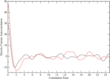
C Electric current autocorrelation and conductivity

The last transport property we study in this paper is the electric current autocorrelation and the electric conductivity. This analysis is only done for pure electric M00 plasma since the comparison among M00, M25 and M50 (which already have different E-charge concentrations) doesn’t make much sense. The electric current autocorrelation is given by

$$\sigma(\tau)=\frac{1}{3VT}<(\sum_{i=1}^{N}e_{i}\vec{v}_{i}(\tau))\cdot(\sum_{i=1}^{N}e_{i}\vec{v}_{i}(0))>$$ (52)

with $e_{i}$ the electric charge of the $i$th particle. And the electric conductivity is obtained from Kubo formula as

$$\sigma=\int_{0}^{\infty}\sigma(\tau)d\tau$$ (53)

In Fig.17 we show the typical $\sigma(\tau)$ as a function of $\tau$ for two values of $\Gamma$. For this correlation function we do notice that even for $\Gamma$ not large, the late time correlation is not purely noise but still has small oscillation. This is not unreasonable since related collective modes like plasmon may develop even for a gas. After integration it turns out in the region $\Gamma\sim 0.3-15$ the conductivity is scattered between $\sigma=0.101-0.141$ without clear tendency, which may indicate the electric current dissipation is not sensitive to $\Gamma$ in this region. It is very interesting to see what will happen to the color-electric conductivity (giving information about color charge transport) in a Non-Abelian plasma.

FIG. 17.: (color online) Electric current autocorrelation functions $\sigma(\tau)$ for pure electric M00 plasma taken at (from top down at zero time) $\Gamma=6.33$(red curve) and $\Gamma=14.53$(black curve).

D Mapping between MD systems and sQGP

With the MD-obtained empirical formulae for diffusion and viscosity, it is of great interest to see what they predict for the parameter region corresponding to the sQGP experimentally created at RHIC. To do this mapping, one has to identify the corresponding physical values of basic units (namely mass, length and time) in the destination system and then combine dimensionless numbers and relations from MD with proper dimensions. Also the plasma parameter $\Gamma$ should be determined for the destination system such that we pick up the MD-predicted values of interesting quantities (say, diffusion constant and shear viscosity) at exactly the same $\Gamma$ value.

Following similar estimates as in [11], we summarize below the relevant quantities of sQGP around $1.5T_{c}$:
1. Quasiparticle (quarks and gluons) mass can be estimated as $m\approx 3.0T$;
2. The typical length scale is simply estimated from quantum localization to be $r_{0}\approx 1/m\approx 1/(3.0T)$;
3. The electric coupling strength, after averaging over different EQPs(quarks and gluons) with their respective Casimir, is roughly $<\alpha_{s}C>\approx 1$;
4. The particle density is roughly given, under the light that lattice results have shown the sQGP pressure and entropy to reach about 0.8 of Stefan-Boltzmann limit, by $n\approx 0.8(0.122\times 2\times 8+0.091\times 2\times 2\times N_{c}\times N_{f})T^{3}\approx 4.2T^{3}$;
5. This density estimation leads to the Wigner-Seitz radius $a_{WS}=(\frac{3}{4\pi n})^{1/3}\approx 1/(2.6T)\approx 1.1r_{0}$;
6. We then get the time scale as the inverse of plasmon frequency $\tau_{p}=1/\omega_{p}=(\frac{m}{4\pi n\alpha_{s}C})^{1/2}\approx 1/(4.2T)$;
7. The entropy density is estimated from Stefan-Boltzmann limit as $s\approx 0.8\times\frac{4\pi^{2}}{90}[2\times 8+(7/8)\times 2\times 2\times N_{c}\times N_{f}]T^{3}\approx 16T^{3}$.

Now let’s discuss the value of $\Gamma$. As already mentioned, the $\Gamma$ given in our MD is the actual ratio of potential to kinetc energy, which is measured during the simulation. The usually quoted one, defined as $\tilde{\Gamma}=\frac{e^{2}}{a_{WS}(k_{B}T)}$, could be considered as a pre-determined ’superficial Gamma’. Unfortunately it is not clear how to estimate the actual Gamma $\Gamma$ of sQGP while the superficial Gamma $\tilde{\Gamma}$ is obtainable for sQGP, which is $\tilde{\Gamma}\approx 2.6<\alpha_{s}C>\approx 2.6$. So we should try to figure out the superficial Gamma in our MD and map the results accordingly. The two are different though, they are monotonously related to each other, namely when one is large(small) so is the other. Since our MD has been done with $n\lambda^{3}=0.17$, the $(a_{WS})_{MD}\approx 1.12\lambda$ which means in our MD $\tilde{\Gamma}=0.89/T$, which after combination with (34) will give us the convertion formula between the two Gamma’s. Similar convertion relation could also be obtained for cQGP in [11] from their Fig.8 though in their case they use superficial Gamma as basic parameter and measure potential energy from simulation.

FIG. 18.: (color online) Plots of $Log[1/\eta]$ v.s. $Log[1/D]$ for three different plasmas. The shaded region is mapped back from experimental values, see text.

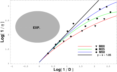
With all the above ingredients we are at place to do the mapping for interesting transport coefficients $D$ and $\eta$ between our MD systems and the sQGP. The mapping is a two-way business: one may map the experimentally suggested values back into corresponding MD numbers, as is done and shown in Fig.18; or one can use the MD-obtained relations to predict the corresponding relations of sQGP after conversion of units, as is shown in Fig.32 and discussed in the summary part. Here let’s focus on MD systems in Fig.18 where a $Log[1/\eta]$ v.s. $Log[1/D]$ is plotted: data points for all three plasmas fall on a universal unit-slope straight line on the left lower part, indicating a small $\Gamma$ gas limit with diffusion and viscosity both proportional to mean free path; all three curves soon deviate from gas limit at larger $\Gamma$ (strong coupling) and become flat in the liquid region; the shaded oval is obtained by mapping back the following experimental values: $\eta/s\approx 0.1-0.3$, $2\pi TD\approx 1-5$, which is clearly not close to gas region but near the liquid region, especially the one of the M50 curve. More about comparison will be given in the summary part at the end of the paper.

VI Collective excitations at very strongly coupled regime

In this section we will report interesting results for collective excitations found at very strongly coupled regime ($\Gamma$ greater than a few tens) of the pure electric (M00) plasma. The signals of these excitations are extraordinarily clear when $\Gamma$ goes to $\sim 100$ or larger. We came to notice these very good modes not in a straight forward way. Instead, these modes have revealed themselves dramatically in some unusual structures of the dynamical correlation functions and their fourier spectra, which we measured first. Only after thinking about possible source of these structures we turned to systematic and direct measurements for certain collective modes, which are found to coincide with correlation functions’ structures in a distinct manner. As mentioned before, in this regime our plasma is like a ”self-holding drop” which has very different collective motions from a plasma in periodic boxes: the latter has the familiar phonon modes while the former is really like a raindrop, having vibration modes like monopole modes, dipole modes, quadruple modes, etc corresponding to different components of density distribution’s spherical harmonics. We will discuss these modes respectively in more details in the following.

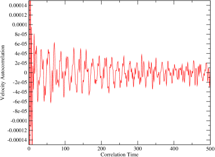
A Monopole modes

Let’s start with the velocity autocorrelation function (37) which is supposed to almost vanish (except a little random noise) at large correlation time and give convergent integral to yield diffusion constant, as seen in previous section. 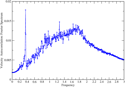However when measured in the very strongly coupled regime, this correlation function is found to have robust oscillating behavior even for very large time which of course couldn’t be considered as noise, see Fig.19. By looking at the fourier spectrum of it, one immediately sees a large and narrow peak at $\omega^{D}_{1}=0.35$ very clearly on top of a very broad shoulder structure, as shown in Fig.20. These behaviors are true for $\Gamma$ down to about $50$.

FIG. 19.: (color online) Velocity autocorrelation function taken at $\Gamma=116.91$.

FIG. 20.: (color online) Fourier transformed spectrum of velocity autocorrelation function taken at $\Gamma=116.91$.

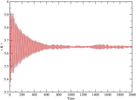
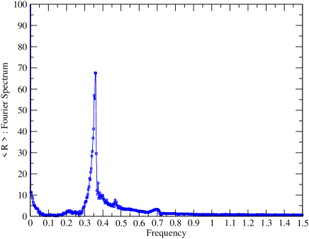
Now the question is why there will be such peaks in velocity autocorrelation. The answer lies in the monopole modes, which can be directly measured through simply the time dependence of average particle radial position, namely:

$$R(t)=\frac{1}{N}\sum_{i=1}^{N}|\vec{r}_{i}(t)|$$ (54)

In Fig.21 one sees really nice oscillations lasting for near hundred revolutions. In a small movie showing the positions of particles at several subsequent time points the ”drop” in monopole mode looks like a beating heat. This oscillation amplitude decreases slowly indicating a nonzero but small width of this monopole mode. Again the fourier spectrum gives important information such as the characteristic frequency and width of collective mode. In Fig.22 we can see one major narrow peak at $\omega^{M}_{1}=0.35$ together with a few roughly visible but much smaller lumps at $\omega=0.22,0.46,0.70$. $\omega=0.70$ structure may be a secondary harmonics of the major peak, and seemingly the $0.22$ and $0.46$ may also be in the same series of harmonics with different ranks.

The important finding we want to point out is the coincidence of $\omega^{M}_{1}$ here with the peak $\omega^{D}_{1}$ from velocity autocorrelation function. This result tells us the monopole mode, in a form of radial vibration, has nontrivial influence on velocity autocorrelation and consequently on particle diffusion.

FIG. 21.: (color online) Average monopole moment $R(t)$ (see text) as a function of time, taken at $\Gamma=116.91$.

FIG. 22.: (color online) Fourier transformed spectrum of average monopole moment $R(t)$(see text), taken at $\Gamma=116.91$.

B Quadruple modes

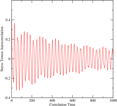
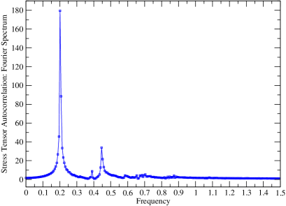
The study of stress tensor autocorrelation in the strongly coupled plasma gives us even more interesting correspondence between correlation functions and collective modes. In Fig.23 we plot the stress tensor autocorrelation (45) as a function of time, and in Fig.24 its fourier spectrum, in which three clear and narrow peaks can be seen at $\omega^{\eta}_{1}=0.20$, $\omega^{\eta}_{2}=0.40$, and $\omega^{\eta}_{3}=0.45$. The $0.40$ peak, which is the smallest one, may be a secondary harmonics of the remarkable $0.20$ peak. At $\Gamma$ as small as about 25, the $0.20$ peak is still alive in this correlation function. Because of the existence of these, the correlation function has significant oscillations with large amplitude even for very large correlation time.

FIG. 23.: (color online) Stress tensor autocorrelation function taken at $\Gamma=116.91$.

FIG. 24.: (color online) Fourier transformed spectrum of stress tensor autocorrelation function taken at $\Gamma=116.91$.

FIG. 25.: (color online) Average off-diagonal quadruple moment $Q_{23}(t)$ (see text) as a function of time, taken at $\Gamma=116.91$.

FIG. 26.: (color online) Fourier transformed spectrum of average off-diagonal quadruple moment $Q_{23}(t)$ (see text), taken at $\Gamma=116.91$.

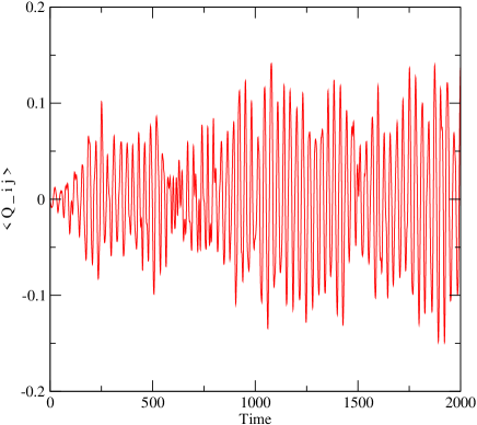
To find the source of these, we directly measured the off-diagonal quadruple modes by the following probe:

$$Q_{lk}(t)=\frac{1}{N}\sum_{i=1}^{N}(\vec{r}_{i}(t))_{l}(\vec{r}_{i}(t))_{k}\quad,\,l,k=1,2,3,\quad l\neq k$$ (55)

We have three independent of them, say $Q_{12},Q_{23},Q_{31}$. In Fig.25 we show one of them as a function of time with similar results for the other two. From the figure we can see that at the very beginning there is almost no quadruple mode but its amplitude grows significantly in a time interval $0-200$ during which the monopole mode decays down (see Fig.21). Then after that they persist for long time. This indicates that these off-diagonal quadruple modes are very robust and somehow ”cheap” to excite and the energy initially in the monopole modes is preferably transferred into the quadruple modes.

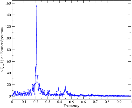
Now when we plot the fourier spectrum of the off-diagonal quadruple modes in Fig.26, amazingly three very clear peaks appear at $\omega^{Q}_{1}=0.20$, $\omega^{Q}_{2}=0.40$, and $\omega^{Q}_{3}=0.45$, which are exactly the same frequencies found in the stress tensor autocorrelation. The relative amplitudes among the three peaks are also similar in two cases. This is a profound correspondence which means the stress tensor correlation and the related transport property, namely viscosity, are especially dominated by the off-diagonal quadruple modes of the system. This type of connection may be universal and one may find certain collective excitations for each dynamical correlation function.

Before closing this subsection, let’s also mention the diagonal quadruple modes which we also studied. This part of quadruples could be probed by the following quantity:

$$Q_{ll}(t)=\frac{1}{N}\sum_{i=1}^{N}{\big{[}}3((\vec{r}_{i}(t))_{l})^{2}-|\vec{r}_{i}(t)|^{2}{\big{]}}\quad,\,l=1,2,3$$ (56)

It has similar behavior as the off-diagonal modes (to save space we skip to show the plots) , with peaks in spectrum at $\omega^{Q}_{4}=0.12$ and $\omega^{Q}_{5}=0.25$ which presumably are different ranks in the same harmonic series. These peaks however are not seen in the stress tensor autocorrelation, which is understandable since the stress tensor autocorrelation we study is actually the correlation of stress tensor’s off-diagonal parts which is related to shear viscosity. We think these peaks of diagonal quadruple modes must be seen in the diagonal parts of stress tensor correlation which is related to the bulk viscosity.

C Plasmon modes

It is clear that our ”drop” won’t have dipole (or any odd-multiple) excitation according to symmetric setting. But there can be another type of dipole excitations, namely the electric dipole modes, or in a more common notion the plasmon modes. These can be probed by

$$(e\vec{R})_{l}(t)=\frac{1}{N}\sum_{i=1}^{N}e_{i}(\vec{r}_{i}(t))_{l}\quad,\,l=1,2,3$$ (58)

FIG. 27.: (color online) Electric current autocorrelation function taken at $\Gamma=116.91$.

FIG. 28.: (color online) Fourier transformed spectrum of electric current autocorrelation function taken at $\Gamma=116.91$.

FIG. 29.: (color online) Average electric dipole moment $eR(t)$ (see text) as a function of time, taken at $\Gamma=116.91$.

FIG. 30.: (color online) Fourier transformed spectrum of average electric dipole moment $eR(t)$ (see text), taken at $\Gamma=116.91$.

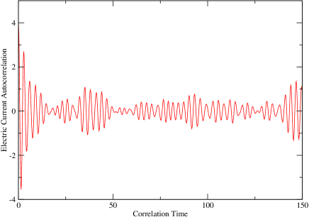
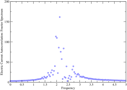
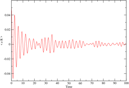
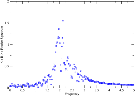
The corresponding correlation function should be the electric current autocorrelation (52). To clearly reveal these modes we shift our positive charges and negative charges with small displacement in opposite directions at the initial time which introduces zero dipole but nonzero electric dipole. We then plot the electric current autocorrelation (Fig.27) and its fourier spectrum (Fig.28), and the direct electric dipole (Fig.29) and its fourier spectrum (Fig.30) as well.

Again one see similar behavior in both and find similar peak structure at $\omega^{J}=\omega^{E}=2.0$ in both spectra. These peaks are large but broad and have some fluctuation, as compared with previous peaks, which is understandable as the plasmon modes usually have bigger width (larger dissipation) than sound modes. These modes seem to be present even if the system has only $\Gamma\sim 10$. If one calculate the plasmon frequency using the simple formula $\omega_{p}=\sqrt{\frac{4\pi ne^{2}}{m}}$ for our drop (with $n=1/a^{3}\,,\,a=1.18\lambda$) we then get $\omega_{p}=2.7$. This is not far from the observed $2.0$ and the discrepancy must be there because the size of our system is only about 10 times the microscopic scale and the positive and negative charges in the middle are not entirely screening each other as assumed when deriving the formula.

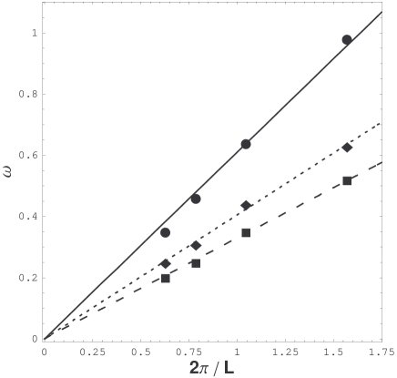
D Size scaling of the collective modes

Since the monopole and quadruple modes should be sound modes, it is interesting to see how their frequencies scale with the system size. For a large enough system one expects the sound modes dispersion to be $\omega=c_{s}k-\frac{i}{2}\Gamma_{s}k^{2}$, namely the mode frequency itself scales linearly in $k$ while the width scales quadratically. What we did is to change system size to be $10\times 10\times 10$, $8\times 8\times 8$, $6\times 6\times 6$, and $4\times 4\times 4$, and then look at the change of peaks in those monopole and quadruple modes (picking the major peaks $\omega^{M}_{1}$, $\omega^{Q}_{1}$ and $\omega^{Q}_{5}$). As demonstrated in Fig.31 where these frequencies are shown as function of $2\pi/L$ with $L$ the system size, the linear scaling is very well observed. We obtain the following linear fitting for the three modes:

$$Monopole\, :\,\omega^{M}_{1}=0.610\,\cdot\,k$$ (59)

$$Quadruple\,D\, :\,\omega^{Q}_{5}=0.404\,\cdot\,k$$ (60)

$$Quadruple\,N-D\, :\,\omega^{Q}_{1}=0.329\,\cdot\,k$$ (61)

The two quadruple modes have similar slope (with the diagonal one a little larger) which means they have close propagation velocity, while the monopole modes have a slope or propagation velocity larger by a factor about $1.5-2$. This is reasonable, just like in usual solid the longitudinal sound waves have larger velocity than the transverse ones. The lines show remarkable consistency with the fact that sound modes with infinitely large wavelength should have zero frequency. For the width however we didn’t unambiguously see a regular dependence on $L$, which indicates our systems are not macroscopic enough since the width is more sensitive than frequency itself to the dissipation effect related to system size.

FIG. 31.: Peak frequency as a function of $2\pi/L$ (with $L$ the system size) for monopole modes(circle), diagonal quadruple modes(diamond), and off-diagonal quadruple modes(square) respectively, with the three lines from linear fitting (see text).

The last result to mention is about the dependence of plasmon modes on system size. Actually we found for all four sizes, the plasmon frequencies roughly stay around $\omega^{E}=2.0$ without changing, only with the peak structure getting worse. Again this is expected since the usual plasmon dispersion displays a plateau at $\omega_{p}=\sqrt{\frac{4\pi ne^{2}}{m}}$ for $k$ not large.

VII Summary and discussion

In summary, we propose to view the finite-$T$ QCD as a competition between electrically charged quasiparticles (EQPs) and the magnetically charged (MQPs). The high-$T$/high density limit is known to be perturbative QGP, which is electric-dominated. This implies that EQPs are more numerous, with density $\sim N_{c}^{2}T^{3}$, while the density of MPQs is $\sim N_{c}^{2}T^{3}/log^{3}(T/\Lambda_{QCD})$. In this case the electric coupling is $weaker$ than the magnetic $e<g$. We think that at some intermediate $T\sim 300\,MeV$ both sectors’ couplings and densities are similar, and below it $T<300\,MeV$ the roles are reversed, with dominant MQPs and electric coupling being $stronger$ than magnetic $e>g$. One of the important consequences of this picture is “postconfinement” phenomena and (electrically) strongly coupled QGP right above the deconfinement phase transition $T=(200-300)\,MeV$.

Using these ideas as a motivation, we start a program of studies aimed at understanding the many-body aspect of matter composed of both of electrically and magnetically charged quasiparticles. (Two-body charge-monopole and charge-dyon situations have been covered in the literature [32, 33].)

Beginning with a 3 body problem: a static E-dipole plus a dynamical monopole, we have found evidences both classically and quantum mechanically that a monopole can be bound to an electric dipole, which will later be more thoroughly treated in a dilute monopole gas scenario and may eventually lead to an explanation of large entropy associated with static quark-anti-quark just above $T_{c}$ as indicated by lattice data.

We have then used molecular dynamics to do the first systematic study of a plasma with both electric and magnetic charges. Two regimes have been separately studied:
1. In the weak and medium coupling regime ($\Gamma<25$), which is most relevant to sQGP problem, the equation of state, the correlation functions and the transport coefficients have been evaluated and compared among plasma with different magnetic contents. Most interestingly we found by increasing the concentration of magnetic charges to about 50% we get a factor $2$ down for viscosity, which is particularly important in view of explaining surprisingly low viscosity of sQGP as observed at RHIC.
2. In the very strongly coupled regime ($\Gamma>25$), very interesting correspondence between correlation functions and collective excitations have been revealed. The monopole modes are found to induce long time oscillation in velocity autocorrelation, while the off-diagonal quadruple modes are shown to have profound dominance on the nontrivial oscillating behavior of stress tensor (off-diagonal) autocorrelation. In a similar manner the plasmon modes are connected to electric current autocorrelation. So with such relation, studying one side also gives us information about the other side. The sound modes nature of such collective excitations has been demonstrated by studying the scaling property of their peak frequencies with system size.

Finally, we would like to compare our results with those obtained using the AdS/CFT correspondence and also with empirical data about sQGP from RHIC experiments. Those are summarized in Fig.32, as a log-log plot of properly normalized dimensionless (heavy quark) diffusion constant and viscosity.

FIG. 32.: (color online) Plots of $Log[1/(\eta/s)]$ v.s. $Log[1/(2\pi TD)]$ including results from our MD simulations, the Ads/CFT calculations, the weakly coupled CFT calculations, as compared with experimental values, see text.

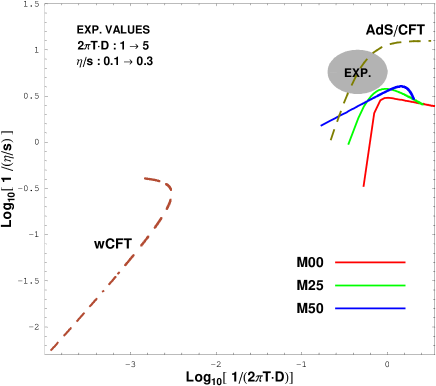
The dashed curve in the left lower corner is for $\cal N$=4 SUSY YM theory in weak coupling, where viscosity is from [41] and diffusion constant from[40]. The curve has a slope of one on this plot, as in weak coupling both quantities are proportional to the same mean free path. As one can easily see, weak coupling results are quite far from empirical data from RHIC, shown by a gray oval in the right upper corner. Viscosity estimates follow from deviations of the elliptic flow at large $p_{t}$ from hydro predictions [38], and diffusion constants are estimated from $R_{AA}$ and elliptic flow of charm [39].

The curve for strong-coupling AdS/CFT results (viscosity according to [42] with $O(\lambda^{-3/2})$ correction, diffusion constant from [35]), shown by upper dashed line, is on the other hand going right through the empirical region. At infinite coupling this curve reaches $s/\eta=4\pi$ which is conjectured to be the ever possible upper bound.

Our results – three solid lines on the right – correspond to our calculations with different EQPs/MQPs ratio. They are close to the empirical region, especially the version with the equal mixture of EQPs and MQPs.

Let us end with a warning, that the empirical data, the mapping from classical system to sQGP and the relation between QCD and the $\cal{N}$ =4 SUSY YM used in AdS/CFT will only become quantitative with time: this figure is just the first attempt to get together all three ingredients of the broad picture.

Acknowledgments.

This work was supported in parts by the US-DOE grant DE-FG-88ER40388. ES thanks A.Vainshtein, E. M.Ilgenfritz and C.Korthals-Altes for helpful discussions.