Lepton asymmetry in the primordial gravitational wave spectrum

Abstract

Effects of neutrino free streaming is evaluated on the primordial spectrum of gravitational radiation taking both neutrino chemical potential and masses into account. The former or the lepton asymmetry induces two competitive effects, namely, to increase anisotropic pressure, which damps the gravitational wave more, and to delay the matter-radiation equality time, which reduces the damping. The latter effect is more prominent and a large lepton asymmetry would reduce the damping. We may thereby be able to measure the magnitude of lepton asymmetry from the primordial gravitational wave spectrum.

I Introduction

Cosmological baryon asymmetry and lepton asymmetry are among the most fundamental quantities of our Universe. The magnitude of baryon asymmetry is determined by two independent methods. Baryon asymmetry can be estimated by comparing the prediction of abundances of the light elements with observations of those quantities in big bang nucleosynthesis (BBN) BBN . The observations of small scale anisotropies of the cosmic microwave background (CMB) also determine the baryon asymmetry. Recent results of the Wilkinson Microwave Anisotropy Probe (WMAP) coincide with the results of BBN within two sigma level WMAP ; WMAP3 . Thus, cosmological baryon asymmetry has been determined very precisely.

On the other hand, lepton asymmetry has still large uncertainties both theoretically and observationally. At very high temperature, sphaleron processes are active, to convert lepton asymmetry to baryon asymmetry and vice versa sphaleron . Then, it is naively expected that the magnitudes of baryon and lepton asymmetry are of the same order through these effects. But, it does not always hold true and many scenarios which allow large lepton asymmetry have been proposed oscillation ; second ; MRM ; KTY ; sp . Then, the determination of the magnitude of lepton asymmetry is crucial to determine cosmic history of our universe. Contrary to the case of baryon asymmetry, however, cosmological lepton asymmetry cannot be observed directly and only upper bounds on lepton asymmetry has been obtained by indirect methods such as BBN, CMB, large scale structure, and so on. The most stringent constraint comes from BBN and the degeneracy parameter $\xi$ is constrained as

$$|\xi_{\nu_{e}}|<0.2\quad{\rm or}\quad|\xi_{\nu_{\mu},\nu_{\tau}}|<2.6$$ (1)

for the case of no mixing HMMMP and

$$|\xi|<0.07$$ (2)

for each family in the case of strong mixing smixing . Here the degeneracy parameter $\xi$ is the ratio of the chemical potential $\mu$ to the (effective) temperature,

$$\xi=\frac{\mu}{T_{\nu}}~{}.$$ (3)

In this paper, we argue that lepton asymmetry may be directly measurable if one can observationally determine the primordial gravitational wave spectrum precisely. During inflation, stochastic gravitational waves are generated and expanded to cosmological scales staro . Then, such gravitational waves memorize all cosmic history during and after inflation, and provide us with fruitful information. For example, the amplitude of the spectrum gives us the energy scale of inflation directly. The spectral shape reflects the history of cosmic expansion: the spectrum is roughly proportional to $f^{-2}$, $f^{0}$, $f$ for the modes which reenter the horizon in the matter dominated phase, the radiation dominated phase, and the kinetic-energy dominated phase. This feature may be used to probe the possible change of the equation of state in the early universe seto . Recently, Watanabe and Komatsu took into account the change of the effective number of degrees of freedom of all standard model particles of particle physics and showed that such changes leave characteristic features in the spectrum WK . Furthermore, Weinberg pointed out that the square amplitude of the gravitational wave is reduced by 35.6% if neutrino free streaming effects are taken into account weinberg .

In this paper, we evaluate neutrino free streaming effects on the primordial gravitational wave spectrum by taking into account lepton asymmetry (chemical potential of neutrinos) and neutrino masses. Lepton asymmetry induces two opposite effects. One is to increase anisotropic pressure, which increases the damping of the spectrum by free streaming effects of neutrinos. The other is to delay the matter-radiation equality, which decreases it. Then, we show that net effect of lepton asymmetry is to decrease the damping of the amplitude of the primordial gravitational wave by free streaming effects of neutrinos.

In the next section, we briefly review the basics of lepton asymmetry and derive anisotropic pressure of neutrino in the presence of lepton asymmetry. In Sec. III, we investigate the evolution of gravitational wave and discuss the damping of the amplitude of the primordial gravitational wave by free streaming effects of neutrinos. Finally we give our discussion and summary.

II Lepton Asymmetric Cosmology

In this section we quickly review the basics of massive degenerate neutrinos. Observational implications of degenerate massive neutrinos for density perturbations have been discussed in the literature LP ; OKMW ; LRV . Here we apply them to the evolution of primordial gravitational wave background.

II.1 background

The energy density of one species of massive degenerate neutrinos and anti-neutrinos is given by FKT ; LP

$$\rho_{\nu}+\rho_{\bar{\nu}} = a^{-4}(k_{B}T_{\nu,0})^{4}\int\frac{d^{3}q}{(2\pi)^{3}}\sqrt{q^{2}+a^{2}m^{2}}\left(f_{\nu}(q)+f_{\bar{\nu}}(q)\right)$$ (4)

$$= (k_{B}T_{\nu})^{4}\int\frac{d^{3}q}{(2\pi)^{3}}\epsilon\left(f_{\nu}(q)+f_{\bar{\nu}}(q)\right)~{}.$$

Here $T_{\nu}$ and $T_{\nu_{0}}$ are the temperature of neutrinos and that of today, respectively, $a$ is a cosmic scale factor, $q$ is comoving momentum in units of $k_{B}T_{\nu,0}$, $m$ is normalized neutrino mass defined by

$$m=\frac{m_{\nu}}{kT_{\nu,0}}~{},$$ (5)

and $\epsilon\equiv\sqrt{q^{2}+a^{2}m^{2}}$ is the comoving energy density. Note that comoving momentum $q$ is related to the proper momentum $p$ by $p=q/a$, which redshifts as $a^{-1}$. Therefore, $q$ is constant relative to the expansion of the universe. When the universe was dense and hot enough, neutrinos were kept in thermal equilibrium with the rest of the plasma through weak interactions so that the distribution function had been relaxed to the form of Fermi-Dirac distribution. Even after neutrino decoupling at $\sim$MeV, owing to Liouville’s theorem, the distribution function is still given by the distribution:

$$f_{\nu}(q)=\frac{1}{1+e^{q-\xi}}~{},\hskip 28.45274ptf_{\bar{\nu}}(q)=\frac{1}{1+e^{q+\xi}}~{}.$$ (6)

Here $\xi$ is the degeneracy parameter.

The pressure is given by

$$3\left(P_{\nu}+P_{\bar{\nu}}\right)=(k_{B}T_{\nu})^{4}\int\frac{d^{3}q}{(2\pi)^{3}}\frac{q^{2}}{\epsilon}\left(f_{\nu}(q)+f_{\bar{\nu}}(q)\right)~{}.$$ (7)

Here and hereafter, we assume that $\mu$ (and $\xi$) is spatially homogeneous for simplicity. In our calculation we also assume, for simplicity, that all the three generations have the same properties, that is, we set $m_{\nu_{e}}=m_{\nu_{\mu}}=m_{\nu_{\tau}}\equiv m_{\nu}$ and $\xi_{\nu_{e}}=\xi_{\nu_{\mu}}=\xi_{\nu_{\tau}}\equiv\xi$.

It will be useful to note the expressions for the energy density and the pressure of massive degenerate neutrinos, in the relativistic and non-relativistic limits for numerical stability and efficiency. In the relativistic limit, the energy density can be written as

$$\rho_{\nu}+\rho_{\bar{\nu}} \approx \frac{(k_{B}T_{\nu})^{4}}{2\pi^{2}}\left[\int q^{3}dq(f_{\nu}+f_{\bar{\nu}})+\int q^{3}dq(f_{\nu}+f_{\bar{\nu}})\frac{(am)^{2}}{2q^{2}}\right]$$ (8)

$$= (\rho_{\nu_{0}}+\rho_{\bar{\nu}_{0}})\left[\left\{1+\frac{30}{7}\left(\frac{\xi}{\pi}\right)^{2}+\frac{15}{7}\left(\frac{\xi}{\pi}\right)^{4}\right\}+\left(\frac{5}{7\pi^{2}}\right)\left\{1+3\left(\frac{\xi}{\pi}\right)^{2}\right\}a^{2}m^{2}\right]~{}.$$

Here we have used the well-known expression for the energy density of massless non-degenerate neutrinos

$$\rho_{\nu_{0}}+\rho_{\bar{\nu}_{0}}=(k_{B}T_{\nu})^{4}\int\frac{d^{3}q}{(2\pi)^{3}}q\frac{2}{1+e^{q}}=\frac{2(k_{B}T_{\nu})^{4}}{2\pi^{2}}\left(\frac{7\pi^{4}}{120}\right)~{}.$$ (9)

In the same manner, the expression for the pressure can be found to be

$$3(P_{\nu}+P_{\bar{\nu}})\approx 2(\rho_{\nu_{0}}+\rho_{\bar{\nu}_{0}})\left\{1+\frac{30}{7}\left(\frac{\xi}{\pi}\right)^{2}+\frac{15}{7}\left(\frac{\xi}{\pi}\right)^{4}\right\}-(\rho_{\nu}+\rho_{\bar{\nu}})~{}.$$ (10)

In the non-relativistic limit, on the other hand, we shall expand $\epsilon$ as $\epsilon\approx am(1+\frac{q^{2}}{2a^{2}m^{2}})$. Unfortunately, we do not have any expression for the even moments of degenerate distribution function in terms of a finite power series of $\xi$. Therefore we keep the integral expressions and write the energy density as

$$\rho_{\nu}+\rho_{\bar{\nu}} \approx \frac{(k_{B}T_{\nu})^{4}}{2\pi^{2}}\left[am\int q^{2}dq(f_{\nu}+f_{\bar{\nu}})+\frac{1}{2am}\int q^{4}dq(f_{\nu}+f_{\bar{\nu}})\right]$$ (11)

$$= (\rho_{\nu_{0}}+\rho_{\bar{\nu}_{0}})\left(am\Theta_{2}+\frac{1}{2am}\Theta_{4}\right)~{},$$

and the pressure as

$$3(P_{\nu}+P_{\bar{\nu}}) \approx \frac{(k_{B}T_{\nu})^{4}}{2\pi^{2}}\left[\frac{1}{am}\int q^{4}dq(f_{\nu}+f_{\bar{\nu}})-\frac{1}{2(am)^{3}}\int q^{6}dq(f_{\nu}+f_{\bar{\nu}})\right]$$ (12)

$$= (\rho_{\nu_{0}}+\rho_{\bar{\nu}_{0}})\left(\frac{1}{am}\Theta_{4}-\frac{1}{2(am)^{3}}\Theta_{6}\right)~{}.$$

Here we have defined the even-moments of distribution function $\Theta_{n}$, normalized by the third moment of non-degenerate fermion distribution, $\int q^{3}dq\frac{2}{(1+e^{q})}=2(\frac{7\pi^{4}}{120})$, as

$$\Theta_{n}(\xi)=\frac{1}{2}\int q^{n}dq(f_{\nu}+f_{\bar{\nu}})\left/\left(\frac{7\pi^{4}}{120}\right)\right.~{}.$$ (13)

Before finishing this subsection we would like to comment on the relation between the cosmological neutrino density parameter $\Omega_{\nu}$ and the mass of a neutrino $m_{\nu}$ FKT .

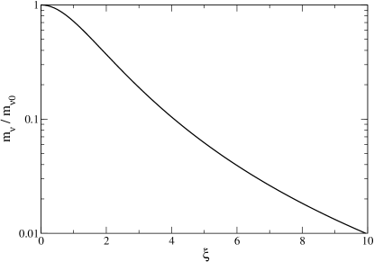
Figure 1: The neutrino mass as a function of $\xi$ normalized by $\xi=0$ non-degenerate neutrino. With $\Omega_{\nu}h^{2}$ fixed, the mass of neutrinos in lepton asymmetric models are lighter than that in symmetric models.

Basically, as long as $m_{\nu}$ is larger than $k_{B}T_{\nu}$, the neutrino mass is related to $\Omega_{\nu}$ as

$$m_{\nu}=\frac{\Omega_{\nu}\rho_{\rm crit}}{N_{\nu}(n_{\nu}+n_{\bar{\nu}})}~{},$$ (14)

where $\Omega_{\nu}$ is the density parameter of neutrinos, $\rho_{\rm crit}$ is the critical density, $N_{\nu}$ is the number of species of massive neutrino, $n_{\nu}$ is the number density of one species of massive neutrino. In the case of degenerate neutrino, the number density is different from that of non-degenerate one, and it is given by

$$(n_{\nu}+n_{\bar{\nu}}) = (k_{B}T_{\nu})^{3}\int\frac{d^{3}q}{(2\pi)^{3}}(f_{\nu}(q)+\bar{f}_{\bar{\nu}}(q))$$ (15)

$$= \frac{(k_{B}T_{\nu})^{3}}{2\pi^{2}}\times 2\left(\frac{7\pi^{4}}{120}\right)\Theta_{2}~{}.$$

By remembering that for non-degenerate massive neutrinos the number density is expressed as

$$(n_{\nu_{0}}+n_{\bar{\nu}_{0}})=\frac{(k_{B}T_{\nu})^{3}}{2\pi^{2}}\times 2\times\frac{3}{2}\zeta(3)~{},$$ (16)

where $\zeta$ is the zeta function, we obtain the following relation between masses of degenerate neutrino and non-degenerate one as

$$\sum m_{\nu}=\frac{\frac{3}{2}\zeta(3)}{\frac{7\pi^{4}}{120}\Theta_{2}(\xi)}\sum m_{\nu_{0}}\left(\frac{T_{\nu}(0)}{T_{\nu}(\xi)}\right)^{3}~{}.$$ (17)

Here $\sum m_{\nu_{0}}=m_{{\nu_{e}}_{0}}+m_{{\nu_{\mu}}_{0}}+m_{{\nu_{\tau}}_{0}}=94.1$ eV $\Omega_{\nu}h^{2}$ is the neutrino mass in the non-degenerate cases, and $T_{\nu}(0)$ and $T_{\nu}(\xi)$ are the present temperatures of standard and degenerate neutrinos, respectively.

The temperatures of degenerate and non-degenerate neutrinos can differ greatly from each other if the chemical potential of neutrinos is so large that neutrinos decouple from the rest of the plasma before muon-antimuon annihilation. In reality, however, neutrinos can be kept in kinetic equilibrium with $e^{\pm}$ even with a significant degeneracy to hold the same temperature as the rest of the plasma until at least the muon-antimuon annihilation ends IK2003 , while number freeze-out can occur before cosmological QCD phase transition KS1992 ; OKMW2 . So, we can safely set $T_{\nu}(0)=T_{\nu}(\xi)=\left(\frac{4}{11}\right)^{1/3}T_{\gamma,0}$ in Eq.(17). Therefore, with the density parameter $\Omega_{\nu}h^{2}$ being fixed, the mass should be monotonically smaller as the neutrinos are degenerate larger. The mass ratio between degenerate and non-degenerate cases is plotted in Fig. 1.

II.2 perturbations

In this paper we only consider the tensor type perturbations. The line element is given by

$$ds^{2}=g_{\mu\nu}dx^{\mu}dx^{\nu}=a^{2}(\tau)\left[-d\tau^{2}+(\delta_{ij}+h^{T}_{ij})dx^{i}dx^{j}\right]~{},$$ (18)

where $h^{T}_{ij}$ denotes tensor type perturbation (gravitational waves) around flat Friedmann-Robertson-Walker metric. We shall work in the transverse traceless gauge, which is set by the conditions $h^{T}_{ij,i}=h^{T}_{ii}=0$. The evolution of gravitational waves $h^{T}_{ij}$ is determined by the linearized Einstein equations:

$$\ddot{h}^{T}_{ij}+2\left(\frac{\dot{a}}{a}\right)\dot{h}^{T}_{ij}+k^{2}h^{T}_{ij}=16\pi Ga^{2}\pi_{ij}~{},$$ (19)

where dots indicate conformal time derivatives, and $\pi_{ij}$ is the anisotropic part of the stress tensor $T_{ij}$, defined by

$$a^{2}\pi_{ij}=T_{ij}-pg_{ij}~{}.$$ (20)

Following the standard procedure, we expand the distribution function of neutrinos into homogeneous and perturbed inhomogeneous parts as

$$f_{\nu}+f_{\bar{\nu}}=(\bar{f}_{\nu}+\bar{f}_{\bar{\nu}})(1+\Psi^{T}(x^{i},\tau,q_{i}))~{}.$$ (21)

Note that we take comoving momentum in the tetrad frame $q_{i}$ as our momentum variable, which is related to the (spatial part of) four momentum $P^{i}$ as $q_{i}=a^{2}P^{j}(\delta_{ij}+\frac{1}{2}h_{ij})$. By virtue of this momentum variable, one can express the moments of distribution function such as energy density, pressure and anisotropic stress in a simple manner, i.e., $q_{i}$ can be treated as that on the flat space background. For example, the anisotropic stress of neutrinos can be written as

$$\pi^{T}_{ij}=(kT_{\nu})^{4}\int\frac{d^{3}q}{(2\pi)^{3}}\frac{q^{2}}{\epsilon}(\gamma_{i}\gamma_{j}-\frac{1}{3}\delta_{ij})(f_{\nu}+f_{\bar{\nu}})\Psi^{T}$$ (22)

where we write the comoving momentum $q_{i}$ in terms of its magnitude and direction: $q_{i}=q\gamma_{i}$, with $\delta^{ij}\gamma_{i}\gamma_{j}=1$.

The perturbed distribution function $\Psi^{T}$ satisfies tensor type collisionless Boltzmann equation in $k$-space

$$\frac{\partial\Psi^{T}_{k}}{\partial\tau}+i\frac{q}{\epsilon}k\mu\Psi^{T}_{k}-\frac{1}{2}\dot{h}_{ij}\gamma^{i}\gamma^{j}\frac{d\ln(\bar{f}_{\nu}+\bar{f}_{\bar{\nu}})}{d\ln q}=0~{},$$ (23)

where $\mu$ is a directional cosine between $\vec{k}$ and $\vec{q}$, and logarithmic derivative of the distribution function with respect to $q$ is given by

$$\frac{d\ln(\bar{f}_{\nu}+\bar{f}_{\bar{\nu}})}{d\ln q}=-\frac{q}{e^{-q}+\cosh\xi}\left(\frac{1+\cosh\xi\cosh q}{\cosh\xi+\cosh q}\right)~{}.$$ (24)

One finds the solution of Eq.(23) as

$$\Psi^{T}=\frac{1}{2}\frac{d\ln(\bar{f}_{\nu}+\bar{f}_{\bar{\nu}})}{d\ln q}\gamma^{i}\gamma^{j}\int^{u}_{0}du^{\prime}e^{i\mu(u^{\prime}-u)}h^{\prime}_{ij}(u^{\prime})~{},$$ (25)

where new time variable $u$ is introduced by

$$u=u(q)\equiv k\int^{\tau}_{\tau_{\rm dec}}\frac{d\tau^{\prime}}{\sqrt{1+\frac{a^{2}m^{2}}{q^{2}}}}~{}.$$ (26)

One of the effects of finite mass comes through Eq.(26), which delays the timing of new time variable $u$ compared with the conformal time $k\tau$.

By inserting the solution Eq.(25) into Eq.(22), and integrating by parts, one obtains

$$\pi^{T}_{ij}=-\frac{(k_{B}T_{\nu})^{4}}{16}\int\frac{q^{2}dq}{2\pi^{2}}(\bar{f}_{\nu}+\bar{f}_{\bar{\nu}})\frac{q^{2}}{\epsilon}\left(5-\frac{q^{2}}{\epsilon^{2}}\right)\int^{u(q)}_{0}du^{\prime}\int^{1}_{-1}dxe^{ix(u-u^{\prime})}(1-x^{2})^{2}\frac{\partial}{\partial u^{\prime}}h_{ij}(u^{\prime})$$ (27)

One can easily confirm that, in cases of massless non-degenerate neutrinos, Eq.(27) reduces to the results obtained in weinberg ; WK . By substituting this expression into the l.h.s. of Eq.(19), one sees that the evolution of gravitational waves is given by solving an integro-differential equation.

In order to see how neutrino asymmetry affects the evolution of gravitational waves, let us first consider massless degenerate neutrinos. When $m=0$, the expression for $\pi^{T}_{ij}$ reduces to

$$\pi^{T}_{ij,\mbox{\scriptsize massless}}=-4(\rho_{\nu}+\rho_{\bar{\nu}})\int^{u}_{0}du^{\prime}\int^{1}_{-1}dx\frac{(1-x^{2})^{2}}{16}e^{ix(u-u^{\prime})}\frac{\partial}{\partial u^{\prime}}h^{T}_{ij}(u^{\prime})~{}.$$ (28)

In such cases, therefore, $q$ dependence of the distribution functions (Eq. (24)) can be integrated away into the energy density, just like in the non-degenerate cases. So the effect of $\xi$ arises only through the background energy density (in the first term of Eq. (8)), and is completely described by introducing an effective number of massless non-degenerate neutrinos.

For massive degenerate neutrinos, however, the situation is quite different. One can no longer express the momentum integration in Eq. (27) in terms of well-known moments such as density, pressure and so on. In other words, it will not be possible to renormalize the dependence of $\xi$ by the effective number of massless non-degenerate neutrinos. Thus, in principle, these two contributions are distinguishable.

In the relativistic limit, the expression of $\pi^{T}_{ij}$ can be expanded to

$$\pi^{T}_{ij} \approx -(k_{B}T_{\nu})^{4}\int\frac{q^{2}dq}{2\pi^{2}}(\bar{f}_{\nu}+\bar{f}_{\bar{\nu}})q\left(4-\frac{a^{2}m^{2}}{q^{2}}\right)$$ (29)

$$\qquad\qquad\qquad\times\int^{u}_{0}du^{\prime}\int^{1}_{-1}dxe^{ix(u-u^{\prime})}\frac{(1-x^{2})^{2}}{16}\frac{\partial}{\partial u^{\prime}}h_{ij}(u^{\prime})$$

$$= \pi^{T}_{ij,\mbox{\scriptsize massless}}+a^{2}m^{2}(\rho_{\nu_{0}}+\rho_{\bar{\nu}_{0}})\left(\frac{10}{7\pi^{2}}\right)\left\{1+3\left(\frac{\xi}{\pi}\right)^{2}\right\}$$

$$\qquad\qquad\qquad\times\int^{u}_{0}du^{\prime}\int^{1}_{-1}dxe^{ix(u-u^{\prime})}\frac{(1-x^{2})^{2}}{16}\frac{\partial}{\partial u^{\prime}}h_{ij}(u^{\prime})~{}.$$

In the non-relativistic limit, on the other hand, $\pi^{T}_{ij}$ can be expressed as

$$\pi^{T}_{ij}\approx-\frac{5}{am}\Theta_{4}(\xi)(\rho_{\nu_{0}}+\rho_{\bar{\nu}_{0}})\int^{u}_{0}du^{\prime}\int^{1}_{-1}dxe^{ix(u-u^{\prime})}\frac{(1-x^{2})^{2}}{16}\frac{\partial}{\partial u^{\prime}}h_{ij}(u^{\prime})$$ (30)

For both limits, a finite mass always acts to suppress the anisotropic stress relative to the massless case. One finds that when neutrinos become massive, $q/\epsilon\to 0$, then $\pi^{T}_{ij}\to 0$.

III evolution of gravitational waves

In the absence of neutrino free streaming in which $\pi^{T}_{ij}=0$, the evolution equation of gravitational waves (Eq. (19)) with an appropriate initial condition has well-known analytical solutions: $h\propto j_{0}(k\tau)$ in the radiation dominated era, and $h\propto j_{1}(k\tau)/(k\tau)$ in the matter dominated era. Thus for both eras, the amplitude of gravitational waves diminishes as $a^{-1}$ with oscillations when waves are well inside the cosmic horizon ($k\tau\gg 1$). This is a general feature of waves in an expanding universe.

The main effect of neutrinos on this evolution of gravitational waves is the damping of amplitude by their free streaming weinberg , and it can be significant when the universe is radiation dominated and neutrinos are relativistic. Because the gravitational waves with wavenumber $k\mathrel{\mathchoice{\lower 3.6pt\vbox{\halign{$\mathsurround=0pt\displaystyle\hfil#\hfil$\cr>\crcr\sim\crcr}}}{\lower 3.6pt\vbox{\halign{$\mathsurround=0pt\textstyle\hfil#\hfil$\cr>\crcr\sim\crcr}}}{\lower 3.6pt\vbox{\halign{$\mathsurround=0pt\scriptstyle\hfil#\hfil$\cr>\crcr\sim\crcr}}}{\lower 3.6pt\vbox{\halign{$\mathsurround=0pt\scriptscriptstyle\hfil#\hfil$\cr>\crcr\sim\crcr}}}}0.01$ Mpc^-1 enter the Hubble horizon before matter-radiation equality for the case of standard massless neutrinos, they suffer from significant damping. This condition holds true unless mass of neutrinos is heavier than $\sim 1$ eV, in which cases neutrinos become non-relativistic before the equality. On the contrary, the gravitational waves with longer wavenumber $k\mathrel{\mathchoice{\lower 3.6pt\vbox{\halign{$\mathsurround=0pt\displaystyle\hfil#\hfil$\cr<\crcr\sim\crcr}}}{\lower 3.6pt\vbox{\halign{$\mathsurround=0pt\textstyle\hfil#\hfil$\cr<\crcr\sim\crcr}}}{\lower 3.6pt\vbox{\halign{$\mathsurround=0pt\scriptstyle\hfil#\hfil$\cr<\crcr\sim\crcr}}}{\lower 3.6pt\vbox{\halign{$\mathsurround=0pt\scriptscriptstyle\hfil#\hfil$\cr<\crcr\sim\crcr}}}}0.01$ Mpc^-1 are not significantly affected by neutrinos. Examples of evolutions of gravitational waves with wavenumbers $k=0.005$, $0.5$ Mpc^-1 are illustrated in Fig. 2.

In Fig. 2, we also show the effect of non-zero chemical potential on the evolution of gravitational waves. Non-zero chemical potential modifies the evolution of gravitational waves mainly in two ways through an effective increase of energy density of neutrinos. One is an effective increase of anisotropic stress in Eq. (28). This increases the effect of free streaming neutrinos, and consequently, the damping of gravitational waves becomes larger. The effect is clearly seen in the numerical evolution of gravitational waves (black dash-dotted line) in Fig. 2. The other is the shift of matter-radiation equality to the later time in the history of the expanding universe. This indirectly gives rise to an overall increase in amplitude of gravitational waves at present for modes which have come across the horizon in the radiation dominated universe.

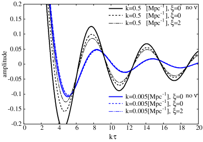
Figure 2: The effects of neutrino free streaming and $\xi$ in the time evolution of gravitational waves. The black lines show the numerical solutions of gravitational waves with wavenumber $k=0.5$ Mpc^-1, and blue (gray) lines show those with wavenumber $k=0.005$ Mpc^-1. The two thickest lines are solutions without neutrinos (no $\nu$). The dash-dotted lines are numerical solutions with degeneracy parameter $\xi=2$. The straight thick and dashed lines are those without chemical potentials. The lines with smaller wavenumber ($k=0.005$) are almost indistinguishable in this figure.

Let us quantitatively discuss the former effect first. An analytic estimation of the damping of gravitational waves by neutrino free streaming was given by DR in a sophisticated way. Here we follow their argument and apply it to the lepton asymmetric cosmology. They expanded a solution of gravitational waves $h(u)$ in a series of spherical Bessel functions as

$$h(u)=\sum_{n=0}^{\infty}a_{n}j_{n}(u)~{}.$$ (31)

At sufficiently late times, the amplitude of gravitational waves asymptotically takes of the form

$$h(u)=A\sin(u+\delta)/u$$ (32)

For large argument, all of the even order Bessel functions go as $\pm\sin x/x$ so the damping factor $A$ is given by

$$A\approx\sum_{n=0}^{5}(-1)^{n}a_{2n}~{}.$$ (33)

Coefficients $a_{2n}$ are determined by the recursion relation

$$a_{2n}=-1.6f_{\nu}\frac{\sum_{k=0}^{n-1}a_{2k}c_{2k,2n-2k}}{2n(2n+1)+1.6f_{\nu}}~{},$$ (34)

starting with $a_{0}=1$, where $f_{\nu}$ is the fraction of the energy density in neutrinos. Numerical coefficients $c_{2k,2n-2k}$ are listed in DR .

For the standard (massless and non-degenerate) neutrinos, $f_{\nu}=0.40523$, which gives $A=0.80313$ DR . However, in the lepton asymmetric cosmology, it is not true in general. Using degeneracy parameter $\xi$, the fraction of the energy density in neutrinos is now given by

$$f_{\nu}(\xi)=\frac{F(\xi)}{F(\xi)+1.46773}~{},$$ (35)

where

$$F(\xi)=1+\frac{30}{7}\left(\frac{\xi}{\pi}\right)^{2}+\frac{15}{7}\left(\frac{\xi}{\pi}\right)^{4}~{}.$$ (36)

When $\xi=\pi$, we get $A\approx 0.64231$. This enhancement of damping by neutrino free streaming is illustrated in Fig. 3.

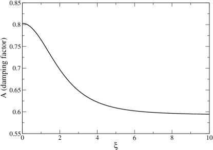
Figure 3: The damping factor as a function of degeneracy parameter $\xi$. The damping effect by neutrino free streaming becomes larger with larger $\xi$.

Next, we discuss the second effect, i.e., the shift of matter-radiation equality. This can result in a modification of the spectrum of gravitational waves at present. In order to investigate it, let us introduce the power spectrum of gravitational waves as

$$\Delta_{h}^{2}=\frac{2k^{3}}{2\pi^{2}}\left<|h|^{2}\right>~{}.$$ (37)

In the simplest inflationary models, it is expected that the power spectrum is nearly scale invariant and has the amplitude of $\frac{16}{\pi}\left(\frac{H_{\rm inf}}{m_{\rm pl}}\right)^{2}$, where $H_{\rm inf}$ is the Hubble parameter during inflation. Alternatively, the spectral energy density, $\Omega_{h}(k)\propto k^{2}\Delta_{h}^{2}$, is often used instead of the power spectrum. It has been shown that, as a result of the evolution of gravitational waves from the deep radiation dominated era through the matter dominated era to the present universe, the spectral energy density has a flat spectrum at $k\mathrel{\mathchoice{\lower 3.6pt\vbox{\halign{$\mathsurround=0pt\displaystyle\hfil#\hfil$\cr>\crcr\sim\crcr}}}{\lower 3.6pt\vbox{\halign{$\mathsurround=0pt\textstyle\hfil#\hfil$\cr>\crcr\sim\crcr}}}{\lower 3.6pt\vbox{\halign{$\mathsurround=0pt\scriptstyle\hfil#\hfil$\cr>\crcr\sim\crcr}}}{\lower 3.6pt\vbox{\halign{$\mathsurround=0pt\scriptscriptstyle\hfil#\hfil$\cr>\crcr\sim\crcr}}}}0.01$ Mpc^-1, where the corresponding Fourier modes have come across the cosmic horizon during radiation dominated era, and $k^{-2}$ at $k\mathrel{\mathchoice{\lower 3.6pt\vbox{\halign{$\mathsurround=0pt\displaystyle\hfil#\hfil$\cr<\crcr\sim\crcr}}}{\lower 3.6pt\vbox{\halign{$\mathsurround=0pt\textstyle\hfil#\hfil$\cr<\crcr\sim\crcr}}}{\lower 3.6pt\vbox{\halign{$\mathsurround=0pt\scriptstyle\hfil#\hfil$\cr<\crcr\sim\crcr}}}{\lower 3.6pt\vbox{\halign{$\mathsurround=0pt\scriptscriptstyle\hfil#\hfil$\cr<\crcr\sim\crcr}}}}0.01$ Mpc^-1, where those have crossed the horizon during matter dominated era Allen . We shall discuss the spectrum of gravitational waves in terms of this spectral energy density.

Because the energy density spectrum of gravitational waves, whose corresponding Fourier modes cross the cosmic horizon during the matter dominated epoch, has a slope of $k^{-2}$ if the primordial spectrum was scale invariant, the amplitude will be boosted by a shift of matter-radiation equality, provided that the normalization of overall amplitude of gravitational waves is given at superhorizon scales. The amplification factor is therefore given by,

$$\frac{\Omega_{h}}{\Omega_{h,\rm standard}}=\left(\frac{k_{\rm eq}}{k_{\rm eq,standard}}\right)^{-2}=\frac{2+1.36F(\xi)}{3.36}~{}.$$ (38)

To derive this relation we have used the fact that the redshift at the matter-radiation equality is given by

$$1+z_{\rm eq}=\frac{\rho_{\rm crit}\Omega_{\rm m}}{\rho_{\gamma,0}+\rho_{\nu,0}}=\frac{8.83\times 10^{3}}{2+1.36F(\xi)}\left(\frac{\Omega_{\rm m}h^{2}}{0.11}\right)~{},$$ (39)

and the corresponding comoving wavenumber is therefore

$$k_{\rm eq}=\frac{H_{\rm eq}}{1+z_{\rm eq}}=0.0145\mbox{ [Mpc${}^{-1}$]}\left(\frac{3.36}{2+1.36F(\xi)}\right)^{1/2}\left(\frac{\Omega_{\rm m}h^{2}}{0.11}\right)~{}.$$ (40)

Here $\Omega_{m}$ is total matter density in units of the critical density $\rho_{\rm crit}$, and $\rho_{\gamma,0}$, $\rho_{\nu_{0}}$ are energy densities of photons and neutrinos today. When $\xi=\pi$, $\frac{\Omega_{h}}{\Omega_{h,\rm st}}\approx 3.6$. This indirect amplification of gravitational waves dominates the damping effect discussed earlier. This is illustrated in Fig. 4.

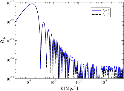
Figure 4: Spectra of gravitational waves with and without lepton asymmetry. The net effect from lepton asymmetry is a rise of the plateau at $k>10^{-2}$ Mpc^-1.

As mentioned earlier, if the mass of neutrinos are heavier than $\sim 1$ eV, neutrinos have gone out from the ultra-relativistic regime before the matter radiation equality and then made their free streaming effect on gravitational waves smaller. In Fig. 5, we depict the effect of finite mass of neutrinos on the time evolution of gravitational waves. From a practical viewpoint, however, the mass of neutrinos as large as $\mathrel{\mathchoice{\lower 3.6pt\vbox{\halign{$\mathsurround=0pt\displaystyle\hfil#\hfil$\cr>\crcr\sim\crcr}}}{\lower 3.6pt\vbox{\halign{$\mathsurround=0pt\textstyle\hfil#\hfil$\cr>\crcr\sim\crcr}}}{\lower 3.6pt\vbox{\halign{$\mathsurround=0pt\scriptstyle\hfil#\hfil$\cr>\crcr\sim\crcr}}}{\lower 3.6pt\vbox{\halign{$\mathsurround=0pt\scriptscriptstyle\hfil#\hfil$\cr>\crcr\sim\crcr}}}}1$ eV is not realistic because even CMB anisotropy data alone by WMAP have already put constraint on the mass as $\sum m_{\nu}\mathrel{\mathchoice{\lower 3.6pt\vbox{\halign{$\mathsurround=0pt\displaystyle\hfil#\hfil$\cr<\crcr\sim\crcr}}}{\lower 3.6pt\vbox{\halign{$\mathsurround=0pt\textstyle\hfil#\hfil$\cr<\crcr\sim\crcr}}}{\lower 3.6pt\vbox{\halign{$\mathsurround=0pt\scriptstyle\hfil#\hfil$\cr<\crcr\sim\crcr}}}{\lower 3.6pt\vbox{\halign{$\mathsurround=0pt\scriptscriptstyle\hfil#\hfil$\cr<\crcr\sim\crcr}}}}2$ eV (at 95% confidence) FIKL and the constraint can be tighter $\sum m_{\nu}\mathrel{\mathchoice{\lower 3.6pt\vbox{\halign{$\mathsurround=0pt\displaystyle\hfil#\hfil$\cr<\crcr\sim\crcr}}}{\lower 3.6pt\vbox{\halign{$\mathsurround=0pt\textstyle\hfil#\hfil$\cr<\crcr\sim\crcr}}}{\lower 3.6pt\vbox{\halign{$\mathsurround=0pt\scriptstyle\hfil#\hfil$\cr<\crcr\sim\crcr}}}{\lower 3.6pt\vbox{\halign{$\mathsurround=0pt\scriptscriptstyle\hfil#\hfil$\cr<\crcr\sim\crcr}}}}0.68$ eV if the information from the matter power spectra is included WMAP3 . Therefore we may conclude that the effect of finite mass of neutrinos cannot be significant on the evolution of gravitational waves.

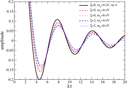
Figure 5: The effects of finite neutrino mass ($m_{\nu}=4$ eV) in the evolution of gravitational waves with the wavenumber $k=0.05$ Mpc^-1. The finite mass suppresses the anisotropic stress of neutrinos and the damping effect becomes smaller.

IV Discussion and Summary

In this paper we investigated the evolution of gravitational wave background in lepton asymmetric cosmology. We showed that the non-zero degeneracy of neutrinos can modify the present spectrum of gravitational wave background through two ways. One is that the non-negligible chemical potential results in the larger anisotropic stress of neutrinos and thus larger damping of amplitude of gravitational waves. The other is the shift of matter radiation equality, which indirectly raises the plateau of the spectrum at $k\mathrel{\mathchoice{\lower 3.6pt\vbox{\halign{$\mathsurround=0pt\displaystyle\hfil#\hfil$\cr>\crcr\sim\crcr}}}{\lower 3.6pt\vbox{\halign{$\mathsurround=0pt\textstyle\hfil#\hfil$\cr>\crcr\sim\crcr}}}{\lower 3.6pt\vbox{\halign{$\mathsurround=0pt\scriptstyle\hfil#\hfil$\cr>\crcr\sim\crcr}}}{\lower 3.6pt\vbox{\halign{$\mathsurround=0pt\scriptscriptstyle\hfil#\hfil$\cr>\crcr\sim\crcr}}}}10^{-2}$ Mpc^-1. These effects can act in the opposite direction from each other. In fact, we showed that the latter effect dominates the former, and the spectrum has a larger power in total than that in the case with non-degenerate neutrinos. These effects follow from the effective increase of number of massless neutrinos. We presented straightforward numerical calculations and analytic estimates for both of the effects.

An important implication of our results is that, should the other cosmological parameters such as $\Omega_{m}h^{2}$, $n_{T}$, $m_{\nu}$ ever be known, one can determine in principle the lepton asymmetry by measuring the gravitational wave amplitude around $k\mathrel{\mathchoice{\lower 3.6pt\vbox{\halign{$\mathsurround=0pt\displaystyle\hfil#\hfil$\cr>\crcr\sim\crcr}}}{\lower 3.6pt\vbox{\halign{$\mathsurround=0pt\textstyle\hfil#\hfil$\cr>\crcr\sim\crcr}}}{\lower 3.6pt\vbox{\halign{$\mathsurround=0pt\scriptstyle\hfil#\hfil$\cr>\crcr\sim\crcr}}}{\lower 3.6pt\vbox{\halign{$\mathsurround=0pt\scriptscriptstyle\hfil#\hfil$\cr>\crcr\sim\crcr}}}}10^{-2}$Mpc^-1. This fact would become more hopeful noting that, among these cosmological parameters, neutrino mass would not be so important because the mass itself does not affect the shape of the spectrum of gravitational waves once it is constrained to be less than $\sim$ eV from the other cosmological or terrestrial experiments.

Of course, the detection of gravitational wave background is promising but still very challenging. Because the damping due to neutrino free streaming can be found only at lower frequency than $\sim 2\times 10^{-10}$ Hz WK assuming standard decoupling of neutrinos, it will be difficult to detect it in a direct way. Indeed, although the critical frequency would be higher as a consequence of smaller Hubble horizon scale at neutrino decoupling in the presence of a significant degeneracy, the frequency will be still far lower than that aimed by the proposed gravitational wave experiments. The most promising way to measure the lepton asymmetry would be to detect the gravitational wave background indirectly by observing the curl modes of cosmic microwave background polarization patterns. It is expected that, in the future planned experiments of CMB anisotropies such as Planck or CMBpol, the lepton asymmetry would be determined if the degeneracy parameter is as large as $\xi\sim 0.1$ and the contamination from divergence mode of polarization by cosmic shear is cleaned out.

As stated in the introduction, in case that flavor equilibrium between all active neutrino species is established before BBN epoch, which is indicated by the large mixing angle solution of the solar neutrino problem, light element abundances have already put a tight conservative limit on degeneracy parameter as $|\xi|\mathrel{\mathchoice{\lower 3.6pt\vbox{\halign{$\mathsurround=0pt\displaystyle\hfil#\hfil$\cr<\crcr\sim\crcr}}}{\lower 3.6pt\vbox{\halign{$\mathsurround=0pt\textstyle\hfil#\hfil$\cr<\crcr\sim\crcr}}}{\lower 3.6pt\vbox{\halign{$\mathsurround=0pt\scriptstyle\hfil#\hfil$\cr<\crcr\sim\crcr}}}{\lower 3.6pt\vbox{\halign{$\mathsurround=0pt\scriptscriptstyle\hfil#\hfil$\cr<\crcr\sim\crcr}}}}0.1$ smixing . However, because the other solution may exist in which flavor mixing can be achieved only partially smixing , and because the evolutions of CMB anisotropies are completely independent from BBN physics, it will still be important to investigate how much the sensitivity of CMB anisotropies for $\xi$ can be improved by including the effect of $\xi$ on the evolution of gravitational waves studied here.

- (1)
- (2) For review, see E. W. Kolb and M. S. Turner, The Early Universe (Addison-Wesley, New York, 1990); K. A. Olive, G. Steigman, and T. P. Walker, Phys. Rep. 333, 389 (2000); D. Tytler, J. M. O’Meara, N. Suzuki, and D. Lubin, Phys. Scr., T85, 12 (2000).
- (3) C. L. Bennett et al., Astrophys. J., Suppl. Ser. 148, 1 (2003);148, 175 (2003); H. V. Peiris et al., Astrophys. J., Suppl. Ser. 148, 213 (2003).
- (4) D. Spergel et al., astro-ph/0603449.
- (5) S. Yu. Khlebnikov and M. F. Shaposhnikov, Nucl. Phys. B308, 885 (1988); J. A. Harvey and M. S. Turner, Phys. Rev. D 42, 3344 (1990).
- (6) K. Enqvist, K. Kainulainen, and J. Maalampi, Phys. Lett. B 244, 186 (1990); R. Foot, M. J. Thomson, and R. R. Volkas, Phys. Rev. D 53, 5349 (1996); X. Shi, ibid. 54, 2753 (1996); For review and further references, see A. D. Dolgov, Phys. Rep. 370, 333 (2002), Sec. 12.5.
- (7) J. A. Harvey and E. W. Kolb, Phys. Rev. D 24, 2090 (1981); A. Casas, W. Y. Cheng, and G. Gelmini, Nucl. Phys. B538, 297 (1999); J. McDonald, Phys. Rev. Lett. 84, 4798 (2000).
- (8) J. March-Russell, A. Riotto, and H. Murayama, J. High Energy Phys. 11, 015 (1999).
- (9) M. Kawasaki, F. Takahashi, and M. Yamaguchi, Phys. Rev. D 66, 043516 (2002).
- (10) M. Yamaguchi, Phys. Rev. D 68, 063507 (2003); T. Chiba, F. Takahashi, and M. Yamaguchi, Phys. Rev. Lett. 92, 011301 (2004); F. Takahashi and M. Yamaguchi, Phys. Rev. D 69, 083506 (2004).
- (11) S.H. Hansen, G. Mangano, A. Melchiorri, G. Miele, and O. Pisanti, Phys. Rev. D 65, 023511 (2002).
- (12) A.D. Dolgov, S.H. Hansen, S. Pastor, S.T. Petcov, G.G. Raffelt, D.V. Semikoz, Nucl. Phys. B632, 363 (2002).
- (13) K. S. Babu, Phys. Lett. B 275, 112 (1992); L. Bento and Z. Berezhiani, Phys. Rev. D 64, 115015 (2001); A. D. Dolgov and F. Takahashi, Nucl. Phys. B688, 189 (2004);
- (14) A.A. Starobinsky, JETP Lett. 30, 682 (1979).
- (15) N. Seto and J. Yokoyama, J. Phys. Soc. Japan, 72, 3082 (2003).
- (16) Y. Watanabe and E. Komatsu, Phys. Rev. D 73, 123515 (2006).
- (17) D. J. Schwarz, Mod. Phys. Lett. A 13, 2771 (1998); Ann. Phys. 12, 220 (2003)
- (18) S. Weinberg, Phys. Rev. D 69, 023503 (2004).
- (19) J. Lesgourgues and S. Pastor, Phys. Rev. D 60, 103521 (1999).
- (20) M. Orito, T. Kajino, G. J. Mathews and Y. Wang, Phys. Rev. D 65, 123504 (2002).
- (21) M. Lattanzi, R. Ruffini, and G. V. Vereshchagin, Phys. Rev. D 72, 063003 (2005).
- (22) K. Freese, E. W. Kolb, and M. S. Turner, Phys. Rev. D 27, 1689 (1983).
- (23) K. Ichikawa and M. Kawasaki, Phys. Rev. D 67, 063510 (2003)
- (24) H.-S. Kang and G. Steigman, Nucl. Phys. B372, 494 (1992)
- (25) M. Orito, T. Kajino, G. J. Mathews and R. N. Boyd, astro-ph/0005446.
- (26) D. A. Dicus and W. W. Repko, Phys. Rev. D 72, 088302 (2005).
- (27) B. Allen, Some Topics on General Relativity and Gravitational Radiation. Proceedings of the ”Spanish Relativity Meeting ’96”, Valencia, Spain, September 10-13, 1996, edited by J. A. Miralles, J. A. Morales, and D. Saez, 1997., p.3.
- (28) M. Fukugita, K. Ichikawa, M. Kawasaki, O. Lahav, Phys. Rev. D 74, 027302 (2006).