Landau-Zener problem in a three-level neutrino system with non-linear time dependence

Abstract

We consider the level-crossing problem in a three-level system with non-linearly time-varying Hamiltonian (time-dependence $t^{-3}$). We study the validity of the so-called independent crossing approximation in the Landau-Zener model by making comparison with results obtained numerically in density matrix approach. We also demonstrate the failure of the so-called ”nearest zero” approximation of the Landau-Zener level-crossing probability integral.

I Introduction

The Landau-Zener (LZ) model has been widely used for studying the dynamics of two-level quantum systems Landau . When the Hamiltonian of a time dependent system is diagonal, the energy levels would in general cross each other. In the presence of non-diagonal terms (”perturbations”) the crossing is, however, avoided leaving a time-varying non-vanishing gap between the levels. If the gap is sufficiently large, transition between the states is strongly suppressed and the system behaves adiabatically remaining in its particular energy state. However, if the levels get close to each other the adiabaticity may be violated and a transition between the states can take place in the vicinity of the points where the diagonal elements of the Hamiltonian (also called diabatic energies) cross.

The exact analytical solution of the wave equations for this kind of systems can be found only in some special cases. The LZ model offers an approximate method for determining the probability ($P_{\rm LZ}$) of the transitions for two-level crossings by using a quasi-classical approach, essentially the WKB approximation. Originally the LZ-model was applied to transitions in diatomic molecules, but it has later found applications also in nuclear LZNucl and atomic LZatom physics, quantum optics LZopt and laser-driven atoms in time-dependent electric LZelec and magnetic LZmagn fields, as well as in neutrino physics LZneut ; Wolfenstein . Recently the LZ-model has been employed also in problems related to nanostructures nano and Bose-Einstein condensates BEcon .

In contrast to the two-level case, no general approximate solution, i.e. a counterpart of the LZ model, has been found for the level crossing problem of multilevel systems with three or more states. That is, there is no general rule which would estimately tell the state of the multilevel system after the system has passed the level-crossing region when the state of the system before entering the region is given and which would take into account the effect of level crossing. Such theoretically derived rules exist only for some special cases (see e.g.Sinitsyn and references therein).

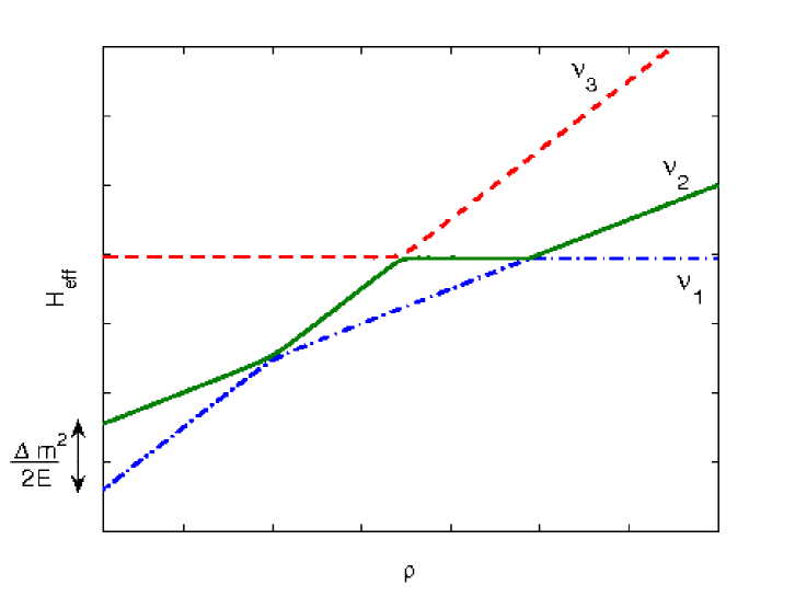
There are also some results which lack mathematical justification but are verified with a high accuracy by numerical studies Smatrix . One such result concerns with a three-level system, where diabatic energies behave all differently as a function of time so that energy levels cross with one another (see Fig. 1). It has been shown numerically that the probability for transitions in this kind of systems can be obtained as a product of the relevant two-state LZ probabilities given that the Hamiltonian describing the system has a linear time dependence. This is what one would expect in the case when the crossing points of diabatic energy levels are well separated, since then only two states at a time are close to each other while the third one is separated from these two with a larger energy gap. What is more surprising is that this simple rule is shown to be valid even when all the crossing points are close to each other Smatrix . That is, the so-called independent crossing approximation works not only in the case where the crossings are well separated but also in the case where they overlap.

In this paper we will study this kind of three-level system in the case of a nonlinear time dependence. We have come across with such a situation when studying evolution of neutrino states in environments where the time dependence of the Hamiltonian is due to a varying density of the background medium KMMR . The matter affects different neutrino types differently, which results in level crossing phenomena. These effects depend on the density distribution of the matter, and they are typically non-linear. We will consider $r^{-3}$ dependence, which is a typical situation in supernovae. This implies the time dependence $t^{-3}$ as light neutrinos are highly relativistic. We will solve the evolution of the three-level system numerically by using the density matrix approach, which we suppose to give the correct description of the behavior of the system. We then make a comparison of the results of the numerical study with the results obtained by the LZ theory and the independent crossing approximation.

II Three-level neutrino system

We will consider a system of the electron neutrino ($\nu_{e}$), another active neutrino ($\nu_{a},a=\mu\,{\rm or}\,\tau$), and a so-called sterile neutrino ($\nu_{s}$). These neutrinos behave differently in a medium: $\nu_{e}$ encounters both charged and neutral current weak interactions, $\nu_{a}$ neutral current interactions only, and $\nu_{s}$ has no interactions with matter at all. The interactions with a medium appears as a ”potential energy” ($V_{e},V_{a},V_{s}$), which is proportional to the density of the matter $\rho$ and the coupling constant of the weak force $G_{F}$ Wolfenstein . The density $\rho$ varies as a function of the location of the neutrino, or the distance $r$ the neutrino has traveled from its creation point.

Figure 1: Diabatic energy levels of a system consisting of the electron neutrino (the steepest straight line), a sterile neutrino (the next steepest line) and the muon or tau neutrino (the horizontal line) in a medium of varying density with normalization defined in the text. Non-diagonal elements of the Hamiltonian makes the system to avoid the crossings making the adiabatic states evolve as indicated by the different line formats in the figure.

The evolution of the system is described by the Schrödinger equation (the Hamiltonian is assumed real for simplicity)

$$i\left(\begin{array}[]{c}\dot{\nu_{e}}\\ \dot{\nu_{s}}\\ \dot{\nu_{a}}\\ \end{array}\right)=\left(\begin{array}[]{ccc}H_{ee}+V_{e}&H_{es}&H_{ea}\\ H_{es}&H_{ss}+V_{s}&H_{sa}\\ H_{ea}&H_{sa}&H_{aa}+V_{a}\\ \end{array}\right)\left(\begin{array}[]{c}\nu_{e}\\ \nu_{s}\\ \nu_{a}\\ \end{array}\right).$$ (1)

The elements $H_{bc}$, which constitute the time-independent part of the Hamiltonian, correspond to the Hamiltonian in vacuum, the non-diagonal elements ($b\neq c$) arising purely from the mixing of neutrino flavours. The neutrino mixing has been observed in experiments through neutrino oscillation phenomena among the neutrinos created in the atmosphere by cosmic rays and among neutrinos originating in the nuclear processes taking place in the core of the Sun. In the following we will not fix our consideration to any particular physical situation but analyze the three-level problem generically.

The $H_{bc}$’s are the elements of the Hamiltonian in vacuum presented in the $(\nu_{e},\nu_{s},\nu_{a})$ flavor basis. They are obtained from

$$U\frac{1}{2E}\left(\begin{array}[]{ccc}m_{1}^{2}&0&0\\ 0&m_{2}^{2}&0\\ 0&0&m_{3}^{2}\\ \end{array}\right)U^{{\dagger}},$$ (2)

where the matrix $U$ can be parameterized in terms of three mixing angles $\theta_{i},i=1,2,3$ as follows:

$$U=\left(\begin{array}[]{ccc}c_{1}c_{3}&s_{1}c_{3}&s_{3}\\ -s_{1}c_{2}-c_{1}s_{2}s_{3}&c_{1}c_{2}-s_{1}s_{2}s_{3}&s_{2}c_{3}\\ s_{1}s_{2}-c_{1}c_{2}s_{3}&-c_{1}s_{2}-s_{1}c_{2}s_{3}&c_{2}c_{3}\\ \end{array}\right),$$ (3)

where $c_{i}=\cos{\theta_{i}}$ and $s_{i}=\sin{\theta_{i}}$. We will consider the mixing angles and neutrino energy as free parameters and we fix their values as is suitable for our purposes.

The mass terms in the diagonal elements of the Hamiltonian result from the relativistic approximation $E_{i}=\sqrt{p^{2}+m_{i}^{2}}\simeq p+m_{i}^{2}/2E$ once the irrelevant overall phase $\exp(ip)$ is omitted. In other words, the behavior of the states in the resonances depends only on the energy differences between the states, not on the absolute values of energies. Similarly, one can also normalize the potential energies. As is common, we will take out the neutral current contribution in a form of an overall phase, leaving the following effective matter potentials for the electron neutrino, the other active neutrinos, and the sterile neutrino, respectively Wolfenstein :

$$V_{e} = \sqrt{2}G_{F}N_{e}$$

$$V_{a} = 0$$ (4)

$$V_{s} = \frac{1}{\sqrt{2}}G_{F}N_{e}.$$

We have assumed ordinary matter where $N_{e}\propto\rho$, and we have for simplicity assumed that $N_{n}=N_{e}$.

The starting point of the LZ approximation is an analytic continuation of the classical action integrals into the complex coordinate plane. In our case this results in the following transition probability between the two states $\nu_{b}$ and $\nu_{c}$ ($b,c=e,s,a$) (in natural units $\hbar=c=1$) Landau

$$P^{LZ}_{bc}=\exp\left[{{-2{\rm Im}\int^{t_{0}}\ {\rm d}t\sqrt{((H_{bb}+V_{b})-(H_{cc}+V_{c}))^{2}+4H_{bc}^{2}}}}\right].$$ (5)

Here $t_{0}$ is a point (a branch point) on the upper half-plane of the complex time, the one nearest to the real time axis, where the quantity under the square root vanishes. The integrand is the energy gap between the two eigenstates (quasi-energies) of the $2\times 2$ sub-Hamiltonian spanned by the states $\nu_{b}$ and $\nu_{c}$. Of course, the eigenstates of the submatrices generally differ from the proper energy eigenstates of the full $3\times 3$ Hamiltonian.

In the case where the time dependence is linear the integral in (5) can be easily solved and the probability is given by the following simple expression Landau :

$$P^{LZ}_{bc}=\exp[{-{\pi\gamma_{bc}}/{2}}],$$ (6)

where the parameter $\gamma_{bc}$ is proportional to the square of the perturbation connecting the states $b$ and $c$, i.e. of $H_{bc}$, and inversely proportional to the slope difference of the unperturbed energy levels at the crossing point $r_{R}$:

$$\gamma_{bc}=\frac{4H_{bc}^{2}}{({d}/{dr})(V_{b}-V_{c})|_{r=r_{R}}}.$$ (7)

In contrast to the linear case, in non-linear cases the integral (5) cannot in general be presented in closed form but one has to evaluate it numerically or approximate it with a suitable series expansion Pantaleone . We will evaluate the integral numerically.

III Results

We now describe the results of our study of the validity of the independent crossing approximation in a three-neutrino case with a non-linear time dependence of energy levels.

We first compute numerically the time evolution of neutrino states using the density matrix formalism. That is, we solve the matrix equation

$$\dot{\rho}=i\left[\rho,H\right],$$ (8)

where $\rho$ is the density matrix. The diagonal elements $\rho_{ee},\>\rho_{ss}$ and $\rho_{aa}$ of the density matrix give the probability for the system with a given initial state at high positive density to end into the states $\nu_{e}$, $\nu_{s}$ and $\nu_{a}$, respectively, at high negative density. Negative density is, of course, just a formal notion; physically, a neutrino at negative density is interpreted as an antineutrino at positive density as the matter potential $V$ has an opposite sign for neutrino and its antiparticle. (In the cases we will consider it will actually be enough to compute the evolution to zero density as no level crossing will take place in negative densities). The relevant contribution to the level crossings is achieved in a limited range where the matter potentials $V_{b}$ ($b=e,s,a$) are of the order of the perturbations $H_{bc}$. The quantity that characterizes the size of this range is the transition width $\delta r_{bc}$, which we define as follows:

$$\delta r_{bc}={\Bigg{|}}\frac{H_{bc}}{(d/dr)(V_{b}-V_{c})|_{r=r_{R}}}{\Bigg{|}}.$$ (9)

When one is well outside this range practically no level crossing takes place but the system remains in the adiabatic energy state.

The ($\nu_{e},\nu_{s},\nu_{a}$) content of the eigenstates of the Hamiltonian of course varies due to the mixing of the neutrinos. The varying ceases when the potential energy terms $V_{b}$ overrule the other terms $H_{bc}$ of the Hamiltonian and the system ends to one of the states $\nu_{e}$, $\nu_{s}$ and $\nu_{a}$ at large negative densities. As no level crossing takes place at negative densities in our case, the flavour states at large negative densities have one-to-one correspondence with mass eigenstates at zero density.

By adjusting the values of the parameters of the Hamiltonian one can move the locations of the crossing points in respect to each other. We have used this in order to test the dependence of the independent crossing approximation on the distance of the crossing points. As far as the crossing points are well separated, that is, their transition width ranges are far from overlapping, the crossings can be clearly considered as independent two-level systems covered by the Landau-Zener model. Then the probability for the level crossing is given by the product of the Landau-Zener probabilities of the two-level crossings on the route.

When the crossing points are so close to each other that their corresponding widths overlap, the situation is different and it is not a priori justified to consider the two-level transitions as independent. Nevertheless, numerical studies show that in the case of linear time-dependence, the independent crossing approximation still gives the correct result Smatrix . We have verified the validity of this result for three-neutrino system in the case of linearly varying matter density. In the following we will study the non-linear case.

We assume that our system consists in the beginning at high matter density from the adiabatic state $\nu_{3}=\nu_{e}$ purely, and we calculate the probability for having the system in the adiabatic state $\nu_{1}$ in the end at zero density (corresponds to the state $\overline{\nu}_{e}$ at large negative density). As one can deduce from Fig. 1, the transition from the adiabatic state $\nu_{3}$ to the adiabatic state $\nu_{1}$ requires non-adiabatic behaviour of the system in two crossings it encounters, i.e. in the 21- and 32-crossings. In the LZ model the probability $P^{LZ}_{31}$ is thus given by

$$P^{LZ}_{31}=P^{LZ}_{32}P^{LZ}_{21}.$$ (10)

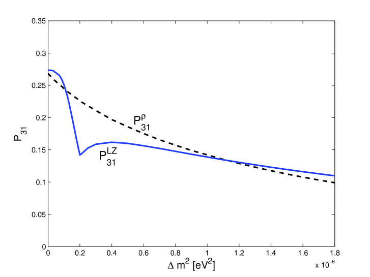
In Fig. 2 we present the probability of the $3\to 1$ transition calculated by the LZ approximation ($P^{LZ}_{31}$) and numerically using the density matrix formalism ($P^{\rho}_{31}$) for different distances between the two crossing points. We have changed the locations of the crossing points by varying the parameter $\Delta m^{2}$, which is the difference between the adiabatic energy states $\nu_{1}$ and $\nu_{2}$ at zero density (see Fig. 1). At high values of $\Delta m^{2}$ the crossing points are well separated and their corresponding transition regions do not overlap. With decreasing $\Delta m^{2}$ the crossing points come closer to each other, and at $\Delta m^{2}=1\times 10^{-6}eV^{2}$ the two transition regions start to overlap. At $\Delta m^{2}=0.5\times 10^{-6}eV^{2}$ the regions are equally wide and overlap completely. At $\Delta m^{2}=0.2\times 10^{-6}eV^{2}$ they are again fully separated.

Figure 2: The probability of the $3\to 1$ transition as a function of the parameter $\Delta m^{2}$ as calculated by using the LZ theory and the independent crossing approximation (solid line) and numerically using the density matrix formalism (dashed line). The two transition regions overlap fully at $\Delta m^{2}=0.5\times 10^{-6}eV^{2}$.

As the plot in Fig. 2 shows, the Landau-Zener model seems to work in our non-linear case relatively well, though underestimating the transition probability to some extent. Anyway, the overlapping of transition regions seems not to dramatically affect the validity of the independent crossing approximation. The situation is actually better than the Fig. 2 indicates, as we will now explain.

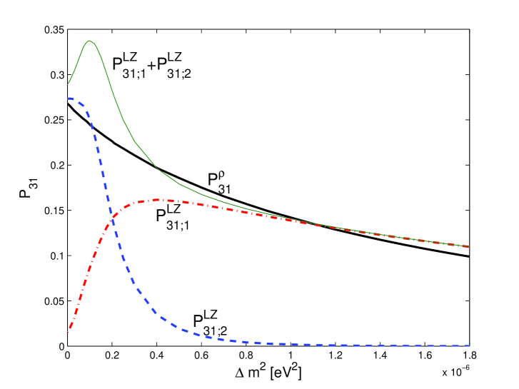
Fig. 2 shows a curious behaviour of $P^{LZ}_{31}$ when $\Delta m^{2}$ is decreased beyond the maximal overlap region. The LZ result seems to be in a serious contradiction with the numerical result of the density matrix approach around the point $\Delta m^{2}=0.2\times 10^{-6}eV^{2}$. This behaviour is actually an artifact of simplistic use of the LZ theory and can be understood as follows. As mentioned, in the integral (5) the upper bound of the integration $t_{0}$ is a point on the upper half-plane of the complex time nearest to the real time axis, where the quasi-energy gap between the two states vanishes. In general, the closest branch point gives the dominant contributions and the contributions of the other branch points with a larger imaginary part are exponentially small, as assumed in the LZ theory.

In our case it happens, however, that at $\Delta m^{2}=0.2\times 10^{-6}eV^{2}$ there are two branch points ($(t_{0})_{1}$ and $(t_{0})_{2}$) with an equal imaginary part, and actually the role of the closest branch point moves from one $t_{0}$ to the other at this value of $\Delta m^{2}$. That is, different $t_{0}$ gives the dominant contribution for large values of $\Delta m^{2}$ than for small values. This is illustrated in Fig. 3, where we plot $P^{LZ}_{31}$ for both of these two zeros. Obviously, the contributions of the both zeros (actually, of all zeros) should be taken into account when evaluating $P^{LZ}_{31}$. It goes beyond the scope of the present work to find out an appropriate way to combine the different contributions coherently (for a discussion on this matter for a two-level systems, see KalleAntti ). Nevertheless, it is quite obvious that once this summation is properly done the odd behaviour of the $P^{LZ}_{31}$ in Fig. 2 will level off and that the the result obtained by the LZ theory and independent crossing approximation gets closer to the numerical result obtained using the density matrix approach than the Fig. 2 shows.

Figure 3: The contributions corresponding to the two dominating branch points $(t_{0})_{1}$ and $(t_{0})_{2}$ to the transition probability $P^{LZ}_{31}$ (dash-dotted and dashed lines, respectively). Also shown are the numerical result obtained by the density matrix approach (thick solid line) and the incoherent sum of the contributions from the two branch points (thin solid line).

IV Conclusions

We have studied in this paper the validity of the independent crossing approximation for a three-level system with non-linear time dependence in the framework of the Landau-Zener model. In particular, we have investigated the case where the transition regions of two level crossings overlap, and we have found that considering the crossings as separate still gives a reasonably good approximation for transition probability as compared with the numerical estimate obtained by using density matrix approach. We have demonstrated also that the simplistic use of the Landau-Zener theory, where the tunneling integral is calculated only for the ”nearest zero” in the complex time plane, leads in some occasions to very inaccurate results.