0.75

KUNS-2044 OHSTPY-HEP-T-06-005 NSF-KITP-06-99 TUM-HEP-650/06 Stringy origin of non-Abelian discrete flavor symmetries

1 Introduction

One of the most important issues in contemporary particle physics is to understand the quark and lepton flavor structure, i.e. the origin of the number of generations, the observed mass hierarchies as well as the mixing angles. Many attempts to understand flavor are based on spontaneously broken Abelian [1] and non-Abelian flavor symmetries [2], such as $S_{3}(\approx D_{3})$ [3], $S_{4}$ [4], $A_{4}$ [5], $D_{4}$ [6], $D_{5}$ [7], $Q_{6}$ [8], $\Delta$-subgroups of SU(3) [9, 10, 11], governing Yukawa couplings for quarks and leptons. Discrete symmetries are not only useful to understand flavor issues (e.g. the observed large mixing angles in the lepton sector) but also to control soft supersymmetry breaking terms, in particular to suppress dangerous flavor changing neutral currents. However, the origin of these discrete symmetries remains obscure in the framework of 4D field theory.

It is not surprising that compactifications of higher-dimensional field theories offer an explanation for the appearance of non-Abelian discrete flavor symmetries, because the latter are symmetries of certain geometrical solids. The symmetries of internal space give rise to symmetries of the interactions between localized fields, which may eventually become flavor symmetries. To be able to evaluate the couplings, and to identify their symmetries, requires the specification of a framework.

We base our analysis on superstring theory, which is a promising candidate for a unified description of nature, including gravity. Consistent (super-)string theories have, in addition to 4D Minkowski space-time, six extra dimensions. An important aspect of string compactifications is that phenomenological features, such as the number of generations and the structure of Yukawa couplings, are determined by geometrical properties of the 6D compact space. 4D string models often enjoy Abelian discrete $\mathbbm{Z}_{N}$ symmetries, which govern the allowed couplings. On the other hand, non-Abelian discrete flavor symmetries derived from string theory have not yet been studied extensively in the literature. The purpose of the present study is to fill this gap.

Among the known string constructions, heterotic orbifold models [12, 13] have a particularly simple geometric interpretation, and an encouraging phenomenology. The selection rules for heterotic orbifolds are well known [14, 15, 16], but little attention has been paid to the emerging non-Abelian flavor symmetries. Recently, explicit string compactifications, based on the $\mathbbm{Z}_{6}\mathrm{-II}=\mathbbm{Z}_{2}\times\mathbbm{Z}_{3}$ heterotic orbifold, with a $D_{4}$ flavor symmetry have been constructed [17, 18, 19, 20]. In these models, the three generations are comprised of a singlet and a doublet under the $D_{4}$ symmetry. This $D_{4}$ flavor symmetry has important phenomenological implications [18, 21].

In this paper we study which types of non-Abelian discrete flavor symmetries can appear in heterotic orbifold models. We classify all the possible non-Abelian discrete symmetries which can arise from heterotic orbifold models, and explore which representations appear in the zero-modes.

The paper is organized as follows. In section 2, we collect some basic facts on strings on orbifolds. Sections 3 and 4 are dedicated to a classification of all the possible non-Abelian discrete flavor symmetries. Their breaking patterns are discussed in section 5. Section 6 is devoted to conclusions and discussion. In appendix A we outline the calculation of coupling strengths on orbifolds. The appendices B and C deal with group-theoretical aspects of $D_{4}$ and $\Delta(54)$.

2 Strings on orbifolds

2.1 Review of basic facts

Let us start with a brief introduction to strings on orbifolds [12, 22] (for recent reviews see [23, 18, 20]). A $d$-dimensional orbifold emerges by dividing a $d$-dimensional torus $\mathbbm{T}^{d}$ by its symmetry, represented by an automorphism (‘twist’) $\theta$. $\mathbbm{T}^{d}$ is obtained as $\mathbbm{R}^{d}/\Lambda$, where $\Lambda$ is a $d$-dimensional lattice, and the twist $\theta$ is the finite-order automorphism of $\Lambda$, i.e. $\theta\,\Lambda=\Lambda$ and $\theta^{N}=\mathbbm{1}$. The orbifold is then denoted as $\mathbbm{T}^{d}/\mathbbm{Z}_{N}$. In other words, $\mathbbm{T}^{d}$ emerges from $\mathbbm{R}^{d}$ through the identification

$$x^{i}~{}\sim~{}x^{i}+n_{a}\,e^{i}_{a}\;,$$ (1)

where $n_{a}$ is integer and $\{e^{i}_{a}\}$ is the lattice basis of $\Lambda$. Furthermore, one identifies points related by $\theta$,

$$(\theta x)^{i}~{}\sim~{}x^{i}+n_{a}\,e^{i}_{a}\;,$$ (2)

on the orbifold. We are specifically interested in 6D orbifolds which preserve N=1 supersymmetry in 4D. For those it is convenient to diagonalize the twist $\theta$, i.e. parametrize $\mathbbm{T}^{6}$ by three complex coordinates $z^{i}$ w.r.t. which

$$\theta~{}=~{}\operatorname{diag}\bigl{(}\exp(2\pi\mathrm{i}\,v_{1}),\exp(2\pi\mathrm{i}\,v_{2}),\exp(2\pi\mathrm{i}\,v_{3})\bigr{)}\;.$$ (3)

Hereby $v_{i}=n_{i}/N$ ($n_{i}\in\mathbbm{Z}$) and $\sum_{i}v_{i}=0$.

Among the Abelian orbifolds, only certain constructions lead to N=1 supersymmetry in 4D. There are, first of all, nine classes of $\mathbbm{Z}_{N}$ orbifolds [12] which are surveyed in table 1 (a). Here the second column shows $v_{i}$ as introduced in (3). Moreover, there are $\mathbbm{Z}_{N}\times\mathbbm{Z}_{M}$ orbifolds which have two independent twists, $\theta$ and $\omega$ with $\theta^{N}=\mathbbm{1}$ and $\omega^{M}=\mathbbm{1}$ (cf. [24]). Nine classes of $\mathbbm{Z}_{N}\times\mathbbm{Z}_{M}$ orbifold models lead to N=1 SUSY. Their twists are shown in table 1 (b) as $\theta=\operatorname{diag}(e^{2\pi\mathrm{i}v^{1}_{1}},e^{2\pi\mathrm{i}v^{1}_{2}},e^{2\pi\mathrm{i}v^{1}_{3}})$ and $\omega=\operatorname{diag}(e^{2\pi\mathrm{i}v^{2}_{1}},e^{2\pi\mathrm{i}v^{2}_{2}},e^{2\pi\mathrm{i}v^{2}_{3}})$. Note that the $\mathbbm{Z}_{2}\times\mathbbm{Z}_{3}$ orbifold is equivalent to the $\mathbbm{Z}_{6}$-II orbifold.

orbifold	twist
$\mathbbm{Z}_{3}$	$(1,1,-2)/3$
$\mathbbm{Z}_{4}$	$(1,1,-2)/4$
$\mathbbm{Z}_{6}$-I	$(1,1,-2)/6$
$\mathbbm{Z}_{6}$-II	$(1,2,-3)/6$
$\mathbbm{Z}_{7}$	$(1,2,-3)/7$
$\mathbbm{Z}_{8}$-I	$(1,2,-3)/8$
$\mathbbm{Z}_{8}$-II	$(1,3,-4)/8$
$\mathbbm{Z}_{12}$-I	$(1,4,-5)/12$
$\mathbbm{Z}_{12}$-II	$(1,5,-6)/12$

(a) $\mathbbm{Z}_{N}$.

orbifold	$v^{1}$	$v^{2}$
$\mathbbm{Z}_{2}\times\mathbbm{Z}_{2}$	$(1,0,-1)/2$	$(0,1,-1)/2$
$\mathbbm{Z}_{2}\times\mathbbm{Z}_{3}$	$(1,0,-1)/2$	$(0,1,-1)/3$
$\mathbbm{Z}_{2}\times\mathbbm{Z}_{4}$	$(1,0,-1)/2$	$(0,1,-1)/4$
$\mathbbm{Z}_{2}\times\mathbbm{Z}_{6}$	$(1,0,-1)/2$	$(0,1,-1)/6$
$\mathbbm{Z}_{2}\times\mathbbm{Z}^{\prime}_{6}$	$(1,0,-1)/2$	$(1,1,-2)/6$
$\mathbbm{Z}_{3}\times\mathbbm{Z}_{3}$	$(1,0,-1)/3$	$(0,1,-1)/3$
$\mathbbm{Z}_{3}\times\mathbbm{Z}_{6}$	$(1,0,-1)/3$	$(0,1,-1)/6$
$\mathbbm{Z}_{4}\times\mathbbm{Z}_{4}$	$(1,0,-1)/4$	$(0,1,-1)/4$
$\mathbbm{Z}_{6}\times\mathbbm{Z}_{6}$	$(1,0,-1)/6$	$(0,1,-1)/6$

(b) $\mathbbm{Z}_{N}\times\mathbbm{Z}_{M}$.

Table 1: (a) $\mathbbm{Z}_{N}$ and (b) $\mathbbm{Z}_{N}\times\mathbbm{Z}_{M}$ orbifold twists for 6D $\mathbbm{Z}_{N}$ orbifolds leading to N=1 SUSY.

Zero-modes, described by string coordinates $X^{i}$, of an orbifold arise from closed strings, satisfying the boundary conditions

$$X^{i}(\sigma+\pi)~{}=~{}(\theta^{k}X)^{i}(\sigma)+n_{a}\,e^{i}_{a}\;.$$ (4)

These boundary conditions can be either untwisted, i.e.  $k=0$, or twisted, i.e. $1\leq k\leq N-1$. Correspondingly, the Hilbert space of (massless) states decomposes in an untwisted and various twisted sectors, denoted by $U$ and $T_{k}$, respectively. The states from the untwisted sector are bulk fields in the effective field theory whereas the twisted states are brane fields living at the fixed points or planes. More specifically, the center-of-mass coordinates of twisted sector zero-modes satisfy an analogous condition to (4),

$$x^{i}~{}=~{}(\theta^{k}x)^{i}+n_{a}\,e^{i}_{a}\;,$$ (5)

and are therefore in one-to-one correspondence to the fixed points or fixed planes of the orbifold. It is common to denote the fixed points or planes by the corresponding space group element $(\theta^{k},n_{a}e^{i}_{a})$. The product of two space group elements, $(\theta^{k^{(1)}},\ell^{(1)})$ and $(\theta^{k^{(2)}},\ell^{(2)})$, is defined by

$$(\theta^{k^{(1)}},\ell^{(1)})\,(\theta^{k^{(2)}},\ell^{(2)})~{}=~{}(\theta^{k^{(1)}+k^{(2)}},\theta^{k^{(1)}}\ell^{(2)}+\ell^{(1)})\;.$$ (6)

Since the orbifold identification implies $\Lambda\sim\theta^{k}\Lambda$, space group elements $(\theta^{k},\ell)$ are only defined up to translations in the sublattice $\Lambda_{k}=(\mathbbm{1}-\theta^{k})\,\Lambda$, i.e. $(\theta,\ell)\simeq(\theta,\ell+(\mathbbm{1}-\theta^{k})\,\lambda)$ with $\lambda\in\Lambda$. In other words, the space group elements appear in conjugacy classes $(\theta^{k},\ell+(\mathbbm{1}-\theta^{k})\,\Lambda)$, and each conjugacy class corresponds to an independent fixed point or plane.

2.2 Couplings on orbifolds

Unlike in the field-theoretic case, coupling strengths are not free parameters in string theory but calculable. In what follows, we give a brief review on Yukawa couplings as well as $n$-point couplings [14, 15, 25].

First of all, couplings in heterotic orbifolds are dictated by selection rules [14, 15, 16, 18, 20]. Apart from gauge invariance and $H$-momentum conservation, allowed couplings are subject to the space group selection rules. An $n$-point coupling among string states corresponding to fixed points $(\theta^{k^{(j)}},\ell^{(j)})$ $(j=1,\cdots,n)$ is allowed only if their product includes the identity,

$$\prod_{j=1}^{n}(\theta^{k^{(j)}},\ell^{(j)})~{}\simeq~{}\bigl{(}\mathbbm{1},0\bigr{)}\;.$$ (7)

Moreover, the coupling strength between localized fields is a function of geometrical features such as the distance between the fields. We review the computation of coupling strengths in appendix A. The important fact for the subsequent discussion is that, if the geometrical settings of two couplings coincide, the coupling strengths coincide as well. In the next sections we shall study the implications of this statement and the space group rule (7).

3 Non-Abelian flavor symmetries of building blocks

In many cases, the torus $\mathbbm{T}^{6}$ factorizes in tori of smaller dimensions, i.e. the lattice $\Lambda$ decomposes in orthogonal sublattices. One is then lead to consider the building blocks

$$\mathbbm{S}^{1}/\mathbbm{Z}_{2}\;,\quad\mathbbm{T}^{2}/\mathbbm{Z}_{3}\;,\ \quad\mathbbm{T}^{2}/\mathbbm{Z}_{4}\;,\quad\mathbbm{T}^{2}/\mathbbm{Z}_{6}\;,\quad\mathbbm{T}^{4}/\mathbbm{Z}_{8}\;,\quad\mathbbm{T}^{4}/\mathbbm{Z}_{12}\;,\quad\mathbbm{T}^{6}/\mathbbm{Z}_{7}\;,$$ (8)

which arise from the 6D orbifold by projection. These building blocks play an important role when discussing orbifold GUT limits [17, 23, 18, 26, 20], where one considers the effective field theory describing anisotropic orbifolds for energies between different compactification scales.

An important property of the space group rule (7) is that, if the torus factorizes, it can be expressed in terms of independent sub-conditions that have to be fulfilled separately for the building blocks. In what follows, we will explain this statement in more detail and study the consequences of rule (7). The discrete flavor symmetries of combinations of building blocks will be studied in section 4.

3.1 $\boldsymbol{\mathbbm{S}^{1}/\mathbbm{Z}_{2}}$ orbifold

In the 1D orbicircle, i.e. the $\mathbbm{S}^{1}/\mathbbm{Z}_{2}$ orbifold (figure 1), there are two independent fixed points, which are denoted by their corresponding space group elements,

$$(\theta,m\,e)\;.$$ (9)

Here $\theta$ is the $\mathbbm{Z}_{2}$ twist (reflection), $m=0,1$ and the $e$ is the unit vector defining $\mathbbm{S}^{1}$, i.e. we identify $x\sim x+e$ on $\mathbbm{R}^{1}$. The sublattice $(\mathbbm{1}-\theta)\Lambda$ is spanned by $2e$. That implies that there are two conjugacy classes corresponding to $(\theta,m\,e)$ with $m$ odd and even. The above space group elements with $m=0,1$ are their representatives.

Figure 1: $\mathbbm{S}^{1}/\mathbbm{Z}_{2}$ orbifold. Points which are related by a reflection on the dashed line are identified. The fundamental region of the orbifold is an interval with the fixed points sitting at the boundaries.

Consequently, there are two types of twisted strings corresponding to the above independent fixed points $(\theta,m\,e)$ with $m=0,1$ (figure 1). In the field-theoretic description, these are brane matter fields living on these fixed points. Let us study the selection rule for allowed $n$-point couplings among twisted states corresponding to $(\theta,m^{(j)}e)$ for $1\leq j\leq n$. Their couplings are allowed when

$$\prod\limits_{j=1}^{n}(\theta,m^{(j)}\,e)~{}=~{}(\mathbbm{1},(\mathbbm{1}-\theta)\Lambda)\;.$$ (10)

The product on the l.h.s. evaluates to

$$\prod\limits_{j=1}^{n}(\theta,m^{(j)}\,e)~{}\simeq~{}(\theta^{n},\sum\limits_{j=1}^{n}m^{(j)}\,e)\;.$$ (11)

Thus, $n$ localized states with the localization described by $(\theta,m^{(j)}\,e)$ can only couple if $n$ and $\sum m^{(j)}$ are even. The latter condition can be understood as a $\mathbbm{Z}_{2}$ symmetry where the twisted state $|(\theta,m^{(j)}),\dots\rangle$ (the omission indicates further quantum numbers) has $\mathbbm{Z}_{2}$ charge $m^{(j)}$. The $\mathbbm{Z}_{2}$ transformation can be represented by

$$\sigma_{3}~{}=~{}\left(\begin{array}[]{cc}1&0\\ 0&-1\end{array}\right)\;,$$ (12)

in a basis where localized states appear as doublets $\left(|(\theta,0),\dots\rangle,|(\theta,e),\dots\rangle\right)$. The requirement that the number $n$ of involved states be even leads to a second $\mathbbm{Z}_{2}$ which acts as $-\mathbbm{1}$ on the above doublets.

Consider, for example, states $x_{i}$ localized at $m=0$, $y_{j}$ localized at $m=1$ and bulk fields $b_{k}$. The symmetries discussed so far restrict allowed couplings to the form

$$x_{i_{1}}\cdots x_{i_{n_{x}}}\,y_{j_{1}}\cdots y_{j_{n_{y}}}\,b_{k_{1}}\cdots b_{k_{n_{b}}}\;,$$ (13)

with $n_{x}$ and $n_{y}$ even. As we shall discuss in the following, one obtains further relations between the coupling strengths from geometry.

These additional relations hold if the background fields (Wilson lines) vanish. Then the two fixed points at $m=0,1$ are equivalent. As a consequence, the Lagrangean is invariant under relabeling $m=0\leftrightarrow 1$. This relabeling can be interpreted as an $S_{2}$ permutation of matter fields localized at the fixed points, and is represented by

$$\sigma_{1}~{}=~{}\left(\begin{array}[]{cc}0&1\\ 1&0\end{array}\right)$$ (14)

in the basis introduced above. This symmetry relates the coupling strengths, i.e. forces the coupling strength of a term of the structure (13) to coincide with an analogous term where $x\leftrightarrow y$. Thus, the flavor symmetry appearing from $\mathbbm{S}^{1}/\mathbbm{Z}_{2}$ is the multiplicative closure of $S_{2}$ and the $\mathbbm{Z}_{2}$s, which is denoted by $S_{2}\cup(\mathbbm{Z}_{2}\times\mathbbm{Z}_{2})$. In the case under consideration, the subgroup $\mathbbm{Z}_{2}\times\mathbbm{Z}_{2}$, generated by $\sigma_{3}$ and $-\mathbbm{1}$, is normal. One can hence write the flavor symmetry as the semi-direct product $S_{2}\ltimes(\mathbbm{Z}_{2}\times\mathbbm{Z}_{2})$. The product of the generators of the two $\mathbbm{Z}_{2}$s and the $S_{2}$ leads to the following elements of the non-Abelian discrete flavor symmetry group:

$$\pm\mathbbm{1}\;,\quad\pm\sigma_{1}\;,\quad\pm\mathrm{i}\sigma_{2}\;,\quad\pm\sigma_{3}\;.$$ (15)

This discrete group is known as $D_{4}\equiv S_{2}\ltimes(\mathbbm{Z}_{2}\times\mathbbm{Z}_{2})$, which is the symmetry of a square.

What we have found so far is that, due to string selection rules and geometry, superpotential terms enjoy a discrete $D_{4}$ symmetry where localized states living at two equivalent fixed points transform as $D_{4}$ doublets ($\boldsymbol{2}$-plets). Bulk fields are trivial $D_{4}$ singlets. Clearly, the introduction of a (discrete) Wilson line breaks this symmetry explicitly to $\mathbbm{Z}_{2}\times\mathbbm{Z}_{2}$.

In conclusion, one can trade the space group selection rule and invariance under relabeling for requiring the Lagrangean to respect a $D_{4}$ ‘flavor’ symmetry. It is important to note that the symmetry of the Lagrangean is larger than the symmetry of internal space. We proceed by applying analogous reasoning to the remaining building blocks (8).

3.2 $\boldsymbol{\mathbbm{T}^{2}/\mathbbm{Z}_{3}}$ orbifold

Let us now consider the $\mathbbm{T}^{2}/\mathbbm{Z}_{3}$ orbifold which emerges by dividing the torus $\mathbbm{T}^{2}_{\mathrm{SU}(3)}$ by its $\mathbbm{Z}_{3}$ rotational symmetry, i.e. the discrete rotation by $120^{\circ}$. Here $\mathbbm{T}^{2}_{\mathrm{SU}(3)}=\mathbbm{R}^{2}/\Lambda_{\mathrm{SU}(3)}$ with $\Lambda_{\mathrm{SU}(3)}$ denoting the $\mathrm{SU}(3)$ root lattice spanned by two simple roots $e_{i}$ ($i=1,2$). The $\mathbbm{Z}_{3}$ twist $\theta$ acts on the lattice vectors as

$$\theta\,e_{1}~{}=~{}e_{2}\;,\quad\theta\,e_{2}~{}=~{}-e_{1}-e_{2}\;.$$ (16)

The sublattice $(1-\theta)\Lambda$ is spanned by $e_{1}-e_{2}$ and $3e_{1}$. There are three independent fixed points under $\theta$, which are represented by

$$(\theta,m_{1}\,e_{1})\;,$$ (17)

with $m_{1}=0,1,2$. The vector $m_{1}\,e_{1}$ is defined up to translations in the sublattice $(1-\theta)\Lambda$.

These twisted states residing on the three equivalent fixed points are degenerate unless the equivalence of the fixed points is lifted by the introduction of non-trivial Wilson lines. Let us consider an $n$-point coupling of twisted matter fields corresponding to $(\theta,m_{1}^{(j)}\,e_{1})$ $(1\leq j\leq n)$. According to (7), this coupling can only be allowed if the product of space group elements,

$$\prod\limits_{j=1}^{n}(\theta,m_{1}^{(j)}\,e_{1})~{}\simeq~{}(\theta^{n},\sum\limits_{j=1}^{n}m_{1}^{(j)}\,e_{1})\;,$$ (18)

is equal to $(\mathbbm{1},(\mathbbm{1}-\theta)\Lambda)$. That requires

$$n~{}=~{}3\times(\mathrm{integer})\;,\qquad\sum\limits_{j=1}^{n}m_{1}^{(j)}~{}=~{}0\mod 3\;.$$ (19)

The first condition is equivalent to demanding that the Lagrangean be invariant under

$$\left(\begin{array}[]{c}|(\theta,0),\dots\rangle\\ |(\theta,e_{1}),\dots\rangle\\ |(\theta,2e_{1}),\dots\rangle\end{array}\right)~{}\to~{}\left(\begin{array}[]{ccc}\omega&0&0\\ 0&\omega&0\\ 0&0&\omega\end{array}\right)\,\left(\begin{array}[]{c}|(\theta,0),\dots\rangle\\ |(\theta,e_{1}),\dots\rangle\\ |(\theta,2e_{1}),\dots\rangle\end{array}\right)\;,$$ (20)

with $\omega=e^{2\pi\mathrm{i}/3}$. The latter condition in (19) corresponds to a $\mathbbm{Z}_{3}$ symmetry where the states with $|(\theta,m_{1}\,e_{1}),\dots\rangle$ have the $\mathbbm{Z}_{3}$ charge $m_{1}$. That is, one requires that the Lagrangean be invariant under the $\mathbbm{Z}_{3}$ transformation

$$\left(\begin{array}[]{c}|(\theta,0),\dots\rangle\\ |(\theta,e_{1}),\dots\rangle\\ |(\theta,2e_{1}),\dots\rangle\end{array}\right)~{}\to~{}\left(\begin{array}[]{ccc}1&0&0\\ 0&\omega&0\\ 0&0&\omega^{2}\end{array}\right)\,\left(\begin{array}[]{c}|(\theta,0),\dots\rangle\\ |(\theta,e_{1}),\dots\rangle\\ |(\theta,2e_{1}),\dots\rangle\end{array}\right)\;.$$ (21)

Furthermore, the effective Lagrangean has an $S_{3}$ permutation (or relabeling) symmetry of the degenerate matter fields living on the three fixed points. Therefore the combination of selection rules and relabeling symmetry leads to a discrete flavor symmetry given by the multiplicative closure $S_{3}\cup(\mathbbm{Z}_{3}\times\mathbbm{Z}_{3})$. As $\mathbbm{Z}_{3}\times\mathbbm{Z}_{3}$ is a normal subgroup, we can write the flavor symmetry group as $S_{3}\ltimes(\mathbbm{Z}_{3}\times\mathbbm{Z}_{3})$. This group has 54 elements and is known as $\Delta(54)$ in the literature (cf. [30]).

Matter fields in the $\mathbbm{Z}_{3}$ orbifold models consist of the untwisted sector $U$ and $\theta$-twisted sector $T_{1}$. The $\theta^{2}$-twisted sector $T_{2}$ contains the anti-particles of $T_{1}$, so that one does not need to treat it separately. The untwisted matter fields transform trivially under $\Delta(54)$. The $T_{1}$ states transform as $\boldsymbol{3}$-plet (while the $T_{2}$ states transform as $\overline{\boldsymbol{3}}$).

In conclusion, the $\mathbbm{T}^{2}/\mathbbm{Z}_{3}$ orbifold (or building block) without Wilson lines enjoys a $\Delta(54)$ flavor symmetry where untwisted and $T_{1}$ states transform as singlet and $\boldsymbol{3}$, respectively.

3.3 $\boldsymbol{\mathbbm{T}^{2}/\mathbbm{Z}_{4}}$ orbifold

To construct the $\mathbbm{T}^{2}/\mathbbm{Z}_{4}$ orbifold we use the torus $\mathbbm{T}^{2}_{\square}$ which is defined by the two orthonormal torus translations $e_{1}$ and $e_{2}$. The $\mathbbm{Z}_{4}$ twist acts on $e_{1}$ and $e_{2}$ as

$$\theta\,e_{1}~{}=~{}e_{2}\;,\qquad\theta\,e_{2}~{}=~{}-e_{1}\;.$$ (22)

There are two independent $\mathbbm{Z}_{4}$ fixed points corresponding to the space group elements

$$(\theta,m_{1}\,e_{1})\;,$$ (23)

with $m_{1}=0,1$ (figure 2).

(a) $\mathbbm{T}^{2}_{\square}/\mathbbm{Z}_{4}$ construction.

(b) $\mathbbm{T}^{2}_{\square}/\mathbbm{Z}_{4}$ triangle.

Figure 2: (a) $\mathbbm{T}^{2}_{\mathrm{SO(5)}}$ is defined by two orthonormal vectors $e_{1}$ and $e_{2}$. There are two $\theta$ fixed points, which are indicated by (blue) squares. In addition one has two $\theta^{2}$ quasi-fixed points (red bullets). The fundamental region of the torus consists of the shaded region, the fundamental region of the orbifold is one quarter thereof. One can fold the fundamental region along the dashed line and identify adjacent edges to obtain a triangle with a fore- and a backside (b).

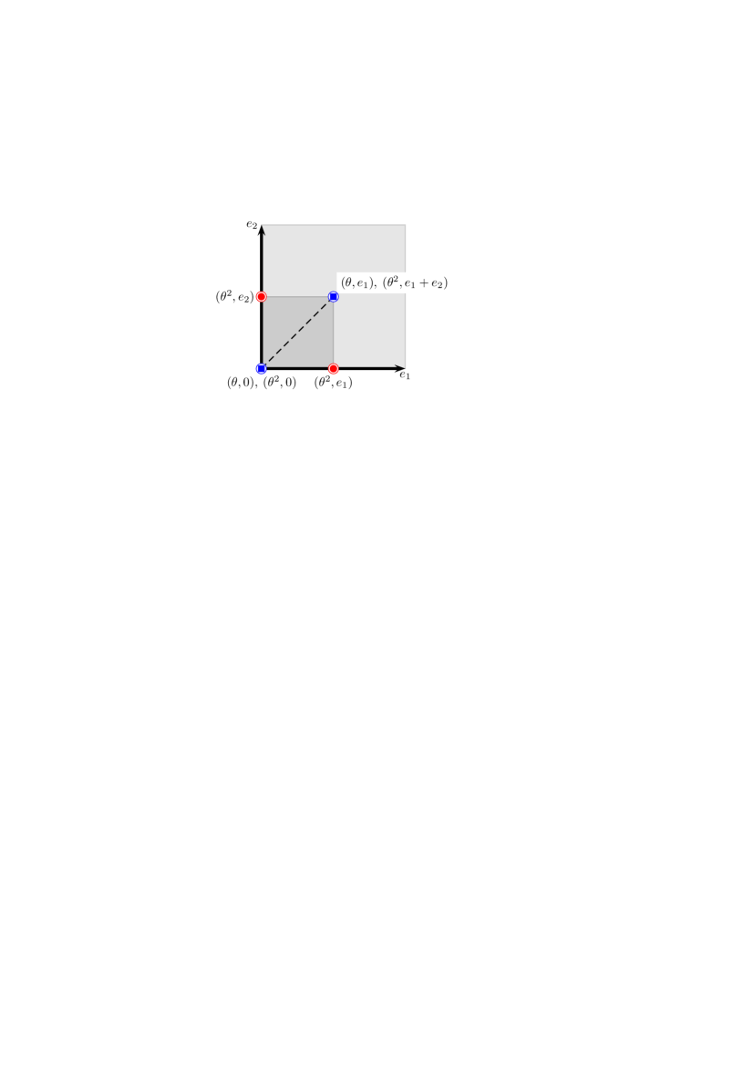
The twisted states decompose into $T_{1}$ and $T_{2}$ twisted sectors, corresponding to the space group elements $(\theta,m_{1}\,e_{1})$ and $(\theta^{2},\sum_{i=1}^{2}m_{i}\,e_{i})$. Let us first discuss $T_{1}$. Consider an $n$-point coupling of twisted matter fields corresponding to $(\theta,m_{1}^{(j)}e_{1})$ $(1\leq j\leq n)$. This coupling is allowed only if the product of space group elements,

$$\prod\limits_{j=1}^{n}(\theta,m_{1}^{(j)}\,e_{1})~{}\simeq~{}(\theta^{n},\sum\limits_{j=1}^{n}m_{1}^{(j)}\,e_{1})\;,$$ (24)

is equal to $(\mathbbm{1},\lambda)$ where $\lambda\in(\mathbbm{1}-\theta)\Lambda$. That requires

$$n~{}=~{}4\times(\mathrm{integer})\;,\qquad\sum_{j}m_{1}^{(j)}~{}=~{}0\mod 2\;.$$ (25)

These conditions imply that the Lagrangean is invariant under the two $\mathbbm{Z}_{4}$ and $\mathbbm{Z}_{2}$ transformations

$$\left(\begin{array}[]{c}|(\theta,0),\dots\rangle\\ |(\theta,e_{1}),\dots\rangle\end{array}\right)~{}\to~{}\left(\begin{array}[]{cc}\mathrm{i}&0\\ 0&\mathrm{i}\end{array}\right)\,\left(\begin{array}[]{c}|(\theta,0),\dots\rangle\\ |(\theta,e_{1}),\dots\rangle\end{array}\right),$$ (26)

$$\left(\begin{array}[]{c}|(\theta,0),\dots\rangle\\ |(\theta,e_{1}),\dots\rangle\end{array}\right)~{}\to~{}\left(\begin{array}[]{cc}1&0\\ 0&-1\end{array}\right)\,\left(\begin{array}[]{c}|(\theta,0),\dots\rangle\\ |(\theta,e_{1}),\dots\rangle\end{array}\right),$$ (27)

respectively. The former is the $\mathbbm{Z}_{4}$ transformation generated by $\mathrm{i}\mathbbm{1}$, while the latter is the $\mathbbm{Z}_{2}$ transformation generated by $\sigma_{3}$. Furthermore, the effective Lagrangean has an $S_{2}$ permutation symmetry generated by $\sigma_{1}$. Thus, the flavor symmetry for $\theta$ twisted states is the multiplicative closure of $\{\mathrm{i}\mathbbm{1},\sigma_{1},\sigma_{3}\}$, denoted by $S_{2}\cup(\mathbbm{Z}_{4}\times\mathbbm{Z}_{2})$. It is quite similar to $D_{4}$, which is the flavor symmetry on $\mathbbm{S}^{1}/\mathbbm{Z}_{2}$. The difference is that the above algebra includes $\mathbbm{Z}_{4}$ elements $\mathrm{i}\mathbbm{1}$ and $-\mathrm{i}\mathbbm{1}$, and their products with $D_{4}$ elements. Note that the element of the $\mathbbm{Z}_{4}$ algebra, $-\mathbbm{1}=(\mathrm{i})^{2}\mathbbm{1}$ is included in the $D_{4}$ algebra. Thus, the flavor symmetry of $\theta$ twisted matter fields is $(D_{4}\times\mathbbm{Z}_{4})/\mathbbm{Z}_{2}$. The division by $\mathbbm{Z}_{2}$ implies that we have to identify the $D_{4}$ element $-\mathbbm{1}$ with the $Z_{4}$ element $(\mathrm{i})^{2}\mathbbm{1}$. This identification has an important meaning for allowed $\mathbbm{Z}_{4}$ charges of $D_{4}$ doublets. If the flavor symmetry was just $D_{4}\times\mathbbm{Z}_{4}$, $D_{4}$ doublets could have an arbitrary $\mathbbm{Z}_{4}$ charge. However, since our flavor symmetry is $(D_{4}\times\mathbbm{Z}_{4})/\mathbbm{Z}_{2}$, the $\mathbbm{Z}_{4}$ charges of $D_{4}$ doublets must be equal to 1 or 3, but not 0 or 2 (mod 4). Hence, the two $T_{1}$ states correspond to $\boldsymbol{2}_{1}$ under $(D_{4}\times\mathbbm{Z}_{4})/\mathbbm{Z}_{2}$. Here, the index denotes the $\mathbbm{Z}_{4}$ charge. There is an ambiguity to assign $\mathbbm{Z}_{4}$ charge 1 or 3 for the $T_{1}$ states, but both assignments are equivalent. With the above assignment, the two $T_{3}$ states correspond to $\boldsymbol{2}_{3}$ under $(D_{4}\times\mathbbm{Z}_{4})/\mathbbm{Z}_{2}$.

Let us now study the $T_{2}$ states. There are four fixed points under the twist $\theta^{2}$,

$$(\theta^{2},m_{1}\,e_{1}+m_{2}\,e_{2})\;,$$ (28)

with $m_{1},m_{2}=0,1$, and there are four corresponding $\theta^{2}$ twisted states,

$$|(\theta^{2},m_{1}\,e_{1}+m_{2}\,e_{2}),\dots\rangle\;.$$ (29)

Note that two fixed points $(\theta^{2},e_{1})$ and $(\theta^{2},e_{2})$ are not fixed points under the $\theta$ twist, but they are transformed into each other, while the other two fixed points are fixed points under the $\theta$ twist. Thus, for states located at $(\theta^{2},e_{1})$ and $(\theta^{2},e_{2})$ one has to take linear combinations to obtain $\theta$ eigenstates as [12, 16]

$$|(\theta^{2},e_{1}),\dots\rangle\pm|(\theta^{2},e_{2}),\dots\rangle\;.$$ (30)

These four space group elements, $(\theta^{2},m_{1}e_{1}+m_{2}e_{2})$, can be obtained as products of two space group elements $(\theta,m_{1}^{(1)}e_{1})$ and $(\theta,m_{1}^{(2)}e_{1})$ according to

$$(\theta^{2},0) =~{}(\theta,0)(\theta,0)\;, \qquad(\theta^{2},e_{1}) =~{}(\theta,e_{1})(\theta,0)\;,$$

$$(\theta^{2},e_{2}) =~{}(\theta,0)(\theta,e_{1})\;, \qquad(\theta^{2},e_{1}+e_{2}) =~{}(\theta,e_{1})(\theta,e_{1})\;.$$ (31)

Since the selection rules for allowed couplings including both $\theta$ twisted states and $\theta^{2}$ twisted states are controlled by the space group, the above products determine how four $\theta^{2}$ twisted states transform under $(D_{4}\times\mathbbm{Z}_{4})/\mathbbm{Z}_{2}$. The two $\theta$ twisted states $|(\theta,m_{1}\,e_{1})),\dots\rangle$ with $m_{1}=0,1$ transform as $\boldsymbol{2}_{1}$ under $(D_{4}\times\mathbbm{Z}_{4})/\mathbbm{Z}_{2}$, and the product of two such doublets yields

$$\boldsymbol{2}_{1}\times\boldsymbol{2}_{1}~{}=~{}(\boldsymbol{1}_{A_{1}})_{2}+(\boldsymbol{1}_{B_{1}})_{2}+(\boldsymbol{1}_{A_{2}})_{2}+(\boldsymbol{1}_{B_{2}})_{2}\;,$$ (32)

where $\boldsymbol{1}_{A_{1},B_{1},A_{2},B_{2}}$ denote the four types of $D_{4}$ singlets (see Appendix B). Thus, four $\theta^{2}$ twisted states can be expressed in terms of four types of $D_{4}$ singlets,

$$(\boldsymbol{1}_{A_{1}})_{2} : |(\theta^{2},0),\dots\rangle+|(\theta^{2},e_{1}+e_{2}),\dots\rangle\;,$$

$$(\boldsymbol{1}_{B_{2}})_{2} : |(\theta^{2},0),\dots\rangle-|(\theta^{2},e_{1}+e_{2}),\dots\rangle\;,$$

$$(\boldsymbol{1}_{B_{1}})_{2} : |(\theta^{2},e_{1}),\dots\rangle+|(\theta^{2},e_{2}),\dots\rangle\;,$$

$$(\boldsymbol{1}_{A_{2}})_{2} : |(\theta^{2},e_{1}),\dots\rangle-|(\theta^{2},e_{2}),\dots\rangle\;.$$ (33)

If we consider couplings including only $\theta^{2}$ twisted states and untwisted states, the flavor symmetry of $\theta^{2}$ twisted states is the same as the discrete symmetry for $T_{1}$ states on $\mathbbm{T}^{2}/\mathbbm{Z}_{2}$, i.e. $(D_{4}\times D_{4})/\mathbbm{Z}_{2}$ (we will discuss this further in section 4.1). However, couplings including both $\theta$ and $\theta^{2}$ twisted states enjoy only $(D_{4}\times\mathbbm{Z}_{4})/\mathbbm{Z}_{2}$.

As an example, let us consider the allowed 3-point couplings, $T_{1}T_{1}T_{2}$. To obtain them, we decompose the product of two $T_{1}$ doublets

$$|\boldsymbol{2}_{1},1\rangle~{}=~{}\left(\begin{array}[]{c}|(\theta,0),1\rangle\\ |(\theta,e_{1}),1\rangle\end{array}\right)\quad\text{and}\quad|\boldsymbol{2}_{1},2\rangle~{}=~{}\left(\begin{array}[]{c}|(\theta,0),2\rangle\\ |(\theta,e_{1}),2\rangle\end{array}\right)$$ (34)

according to (32) into four singlets,

$$\boldsymbol{1}_{A_{1}} : |(\theta,0),1\rangle\,|(\theta,0),2\rangle+|(\theta,e_{1}),1\rangle\,|(\theta,e_{1}),2\rangle\;,$$

$$\boldsymbol{1}_{B_{2}} : |(\theta,0),1\rangle\,|(\theta,0),2\rangle-|(\theta,e_{1}),1\rangle\,|(\theta,e_{1}),2\rangle\;,$$

$$\boldsymbol{1}_{B_{1}} : |(\theta,0),1\rangle\,|(\theta,e_{1}),2\rangle+|(\theta,e_{1}),1\rangle\,|(\theta,0),2\rangle\;,$$

$$\boldsymbol{1}_{A_{2}} : |(\theta,0),1\rangle\,|(\theta,e_{1}),2\rangle-|(\theta,e_{1}),1\rangle\,|(\theta,0),2\rangle\;.$$ (35)

Now seek for invariant product with $T_{2}$ states. Only the following products are invariant:

$$A_{1}\ A_{1},\ A_{2}\ A_{2},\ B_{1}\ B_{1},\ B_{2}\ B_{2}\;.$$ (36)

From $A_{1}^{2}$ and $B_{2}^{2}$ we find the following allowed superpotential terms (we are using the states as synonyms for the superfields)

$$a\ [|(\theta,0),1\rangle\,|(\theta,0),2\rangle+|(\theta,e_{1}),1\rangle\,|(\theta,e_{1}),2\rangle]\ [|(\theta^{2},0)\rangle+|(\theta^{2},e_{1}+e_{2})\rangle]\;,$$

$$b\ [|(\theta,0),1\rangle\,|(\theta,0),2\rangle-|(\theta,e_{1}),1\rangle\,|(\theta,e_{1}),2\rangle]\ [|(\theta^{2},0)\rangle-|(\theta^{2},e_{1}+e_{2})\rangle]\;.$$ (37)

We can re-arrange the couplings above and obtain for the couplings of physical states

$$W \supset c_{1}\,[|(\theta,0),1\rangle\,|(\theta,0),2\rangle\,|(\theta^{2},0)\rangle+|(\theta,e_{1}),1\rangle\,|(\theta,e_{1}),2\rangle\ |(\theta^{2},e_{1}+e_{2})\rangle]$$ (38)

$${}+c_{2}\ [|(\theta,0),1\rangle\,|(\theta,0),2\rangle\,|(\theta^{2},e_{1}+e_{2})\rangle+|(\theta,e_{1}),1\rangle\,|(\theta,e_{1}),2\rangle\,|(\theta^{2},0)\rangle]$$

with $c_{1}=a+b$, $c_{2}=a-b$. From $B_{1}^{2}$ and $A_{2}^{2}$ we get

$$W \supset c\,\left[|(\theta,0),1\rangle\,|(\theta,e_{1}),2\rangle+|(\theta,e_{1}),1\rangle\,|(\theta,0),2\rangle\right]\,[|(\theta^{2},e_{1})\rangle+|(\theta^{2},e_{2})\rangle]$$ (39)

$${}+d\,\left[|(\theta,0),1\rangle\,|(\theta,e_{1}),2\rangle-|(\theta,e_{1}),1\rangle\,|(\theta,0),2\rangle\right]\,[|(\theta^{2},e_{1})\rangle-|(\theta^{2},e_{2})\rangle]\;.$$

The re-arrangement of couplings then analogously reads

$$W \supset c_{3}\,\left[|(\theta,0),1\rangle\,|(\theta,e_{1}),2\rangle\,|(\theta^{2},e_{1})\rangle+|(\theta,e_{1}),1\rangle\,|(\theta,0),2\rangle|(\theta^{2},e_{2})\rangle\right]$$ (40)

$${}+c_{4}\,\left[|(\theta,0),1\rangle\,|(\theta,e_{1}),2\rangle\,|(\theta^{2},e_{2})\rangle+|(\theta,e_{1}),1\rangle\,|(\theta,0),2\rangle\,|(\theta^{2},e_{1})\rangle\right]$$

with $c_{3}=c+d$, $c_{4}=c-d$. The higher-dimensional allowed couplings can be obtained analogously. From the geometry of the setup one infers that $c_{3}=c_{4}$ such that $d=0$ in (39). The vanishing of the $d$-term can also be inferred from gauge invariance. This will be discussed in detail elsewhere.

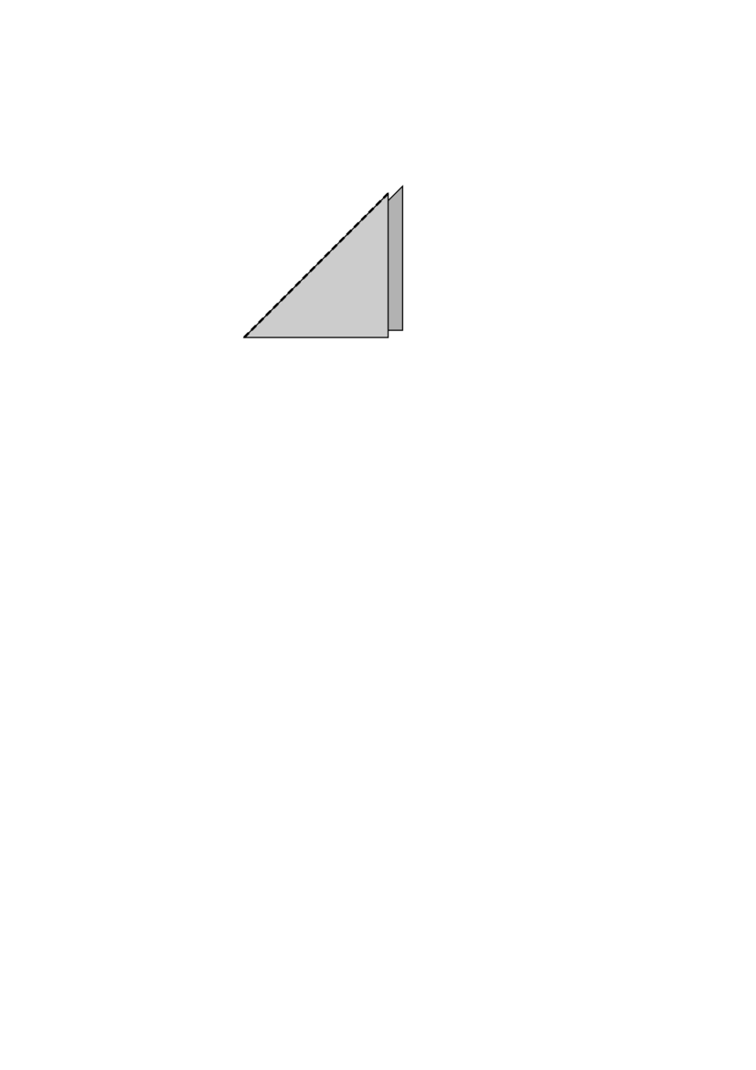
3.4 $\boldsymbol{\mathbbm{T}^{2}/\mathbbm{Z}_{6}}$ orbifold

The 2-dimensional $\mathbbm{Z}_{6}$ orbifold is obtained as $\mathbbm{T}^{2}_{\mathrm{SU}(3)}/\mathbbm{Z}_{6}$. The $\mathbbm{Z}_{6}$ twist is defined for the $\mathrm{SU}(3)$ simple roots $e_{1}$ and $e_{2}$ as

$$\theta\,e_{1}~{}=~{}e_{1}+e_{2}\;,\qquad\theta\,(e_{1}+e_{2})~{}=~{}e_{2}\;,\qquad\theta\,e_{2}~{}=~{}-e_{1}\;.$$ (41)

The sublattice $(1-\theta)\Lambda_{\mathrm{SU}(3)}$ is the same as $\Lambda_{\mathrm{SU}(3)}$. That implies that there is a single (independent) fixed point under the $\mathbbm{Z}_{6}$ twist $\theta$. That is, this orbifold model does not include a non-Abelian flavor structure.

Notice that couplings involving higher twisted sectors only do enjoy non-Abelian discrete symmetries. Analogously to the $\mathbbm{Z}_{4}$ case, these symmetries disappear as soon as $T_{1}$ states enter the couplings.

3.5 $\boldsymbol{\mathbbm{T}^{4}/\mathbbm{Z}_{8}}$ orbifold

The 4-dimensional $\mathbbm{Z}_{8}$ orbifold can be obtained as $\mathbbm{T}^{4}_{\mathrm{SO}(9)}/\mathbbm{Z}_{8}$, where $\mathbbm{T}^{4}_{\mathrm{SO}(9)}$ is the 4-torus based on the SO(9) Lie lattice, which is spanned by the basis vectors $e_{i}$ $(i=1,2,3,4)$. The $\mathbbm{Z}_{8}$ twist transforms the latter

$$\theta\,e_{1}~{}=~{}e_{2}\;,\qquad\theta\,e_{2}~{}=~{}e_{3}\;,\qquad\theta\,e_{3}~{}=~{}\sum_{j=1}^{3}e_{j}+2e_{4}\;,\qquad\theta\,e_{4}~{}=~{}-\sum_{j=1}^{4}e_{j}\;.$$ (42)

The sublattice $(1-\theta)\Lambda$ is spanned by $e_{1},e_{2},e_{3}$ and $2e_{4}$. Thus, there are two fixed points under $\theta$,

$$(\theta,m_{4}\,e_{4}),$$ (43)

for $m_{4}=0,1$.

The flavor symmetry of $T_{1}$ on $\mathbbm{T}^{4}/\mathbbm{Z}_{8}$ is quite similar to the flavor symmetry of $T_{1}$ on $\mathbbm{T}^{2}/\mathbbm{Z}_{4}$. The former is the closure algebra, $S_{2}\cup(\mathbbm{Z}_{8}\times\mathbbm{Z}_{2})$, where $\mathbbm{Z}_{8}$ transforms as

$$\left(\begin{array}[]{c}|(\theta,0),\dots\rangle\\ |(\theta,e_{4}),\dots\rangle\end{array}\right)~{}\to~{}\left(\begin{array}[]{cc}\rho&0\\ 0&\rho\end{array}\right)\,\left(\begin{array}[]{c}|(\theta,0),\dots\rangle\\ |(\theta,e_{4}),\dots\rangle\end{array}\right),$$ (44)

with $\rho=e^{\mathrm{i}\pi/4}$. In addition, $S_{2}$ and $\mathbbm{Z}_{2}$ transformations are represented in the above basis by $\sigma_{1}$ and $\sigma_{3}$, respectively. Thus, the flavor symmetry is written as $S_{2}\cup(\mathbbm{Z}_{8}\times\mathbbm{Z}_{2})=(D_{4}\times\mathbbm{Z}_{8})/\mathbbm{Z}_{2}$, where the division by $\mathbbm{Z}_{2}$ implies that we identify the $D_{4}$ element $-\mathbbm{1}$ with the $\mathbbm{Z}_{8}$ element $\rho^{4}\mathbbm{1}$. Therefore, the two $T_{1}$ states correspond to ${\bf 2}_{1}$ under $(D_{4}\times\mathbbm{Z}_{8})/\mathbbm{Z}_{2}$, where the index denotes $\mathbbm{Z}_{8}$ charge.

In addition, the $\theta^{2}$-twisted sector $T_{2}$ has four independent fixed points,

$$(\theta^{2},m_{3}\,e_{3}+m_{4}\,e_{4}),$$ (45)

with $m_{1},m_{2}=0,1$. Through a discussion similar to section 3.3, we find that four $T_{2}$ states on the above fixed points correspond to four types of singlets,

$$(\boldsymbol{1}_{A_{1}})_{2}+(\boldsymbol{1}_{B_{1}})_{2}+(\boldsymbol{1}_{A_{2}})_{2}+(\boldsymbol{1}_{B_{2}})_{2},$$ (46)

under $(D_{4}\times\mathbbm{Z}_{8})/\mathbbm{Z}_{2}$.

The $\theta^{3}$-twisted sector $T_{3}$ has the same structure of fixed points as the $\theta$-twisted sector. Thus, the two $T_{3}$ states correspond to $\boldsymbol{2}_{3}$ under $(D_{4}\times\mathbbm{Z}_{8})/\mathbbm{Z}_{2}$.

Moreover, the $\theta^{4}$-twisted sector $T_{4}$ has 16 independent fixed points,

$$(\theta^{4},\sum_{i=1}^{4}m_{i}\,e_{i}),$$ (47)

with $m_{i}=0,1$. The corresponding 16 $T_{4}$ states must be $D_{4}$ singlets with the $\mathbbm{Z}_{8}$ charge 4. From the $D_{4}$ multiplication law

$$(\boldsymbol{1}_{A_{1}}+\boldsymbol{1}_{B_{1}}+\boldsymbol{1}_{B_{2}}+\boldsymbol{1}_{A_{2}})\times(\boldsymbol{1}_{A_{1}}+\boldsymbol{1}_{B_{1}}+\boldsymbol{1}_{B_{2}}+\boldsymbol{1}_{A_{2}})~{}=~{}4\times(\boldsymbol{1}_{A_{1}}+\boldsymbol{1}_{B_{1}}+\boldsymbol{1}_{B_{2}}+\boldsymbol{1}_{A_{2}})$$ (48)

it follows that the 16 $T_{4}$ states correspond to

$$4\times\left((\boldsymbol{1}_{A_{1}})_{4}+(\boldsymbol{1}_{B_{1}})_{4}+(\boldsymbol{1}_{B_{2}})_{4}+(\boldsymbol{1}_{A_{2}})_{4}\right)\;.$$ (49)

If we consider couplings involving only $T_{2}$ or $T_{4}$ states, the flavor symmetry would be larger, but it gets broken if $T_{1}$ states enter.

3.6 $\boldsymbol{\mathbbm{T}^{4}/\mathbbm{Z}_{12}}$ orbifold

There is only one fixed point on the $\mathbbm{T}^{4}/\mathbbm{Z}_{12}$ orbifold. Thus, the situation is the same as in $\mathbbm{T}^{2}/\mathbbm{Z}_{6}$, i.e. there is no non-Abelian flavor symmetry.

3.7 $\boldsymbol{\mathbbm{T}^{6}/\mathbbm{Z}_{7}}$ orbifold

For completeness let us consider the $\mathbbm{T}^{6}_{\mathrm{SU}(7)}/\mathbbm{Z}_{7}$ orbifold. It is obtained as $\mathbbm{R}^{6}/(\Lambda_{\mathrm{SU}(7)}\times\mathbbm{Z}_{7})$, where $\Lambda_{\mathrm{SU}(7)}$ denotes the $\mathrm{SU}(7)$ root lattice spanned by six simple roots, $e_{i}$ $(1\leq i\leq 6)$. The $\mathbbm{Z}_{7}$ twist transforms these roots as

$$\theta e_{i}~{}=~{}e_{i+1}\;,\qquad e_{6}~{}=~{}-\sum_{j=1}^{6}e_{j}\;,$$ (50)

for $1\leq i\leq 5$. The sublattice $(1-\theta)\,\Lambda$ is spanned by $e_{i}-e_{i+1}$ and $7e_{1}$, and there are seven independent fixed points under $\theta$,

$$(\theta,m\,e_{1})\;,$$ (51)

with $0\leq m\leq 6$. The other $T_{k}$ sectors with $k\neq 0$ have the same fixed point structure.

The flavor symmetry is obtained in a way similar to the extension of the $\mathbbm{Z}_{3}$ orbifold. That is, the states at these seven fixed points have $\mathbbm{Z}_{7}$ charges, and the effective Lagrangean has a permutation symmetry of $S_{7}$. Therefore, the flavor symmetry of the $\mathbbm{Z}_{7}$ orbifold is the multiplicative closure of $S_{7}$ and the $\mathbbm{Z}_{7}$. To determine the dimension of this group, it is useful to rewrite it as a semi-direct product. It is easy to see that the diagonal matrices corresponding to $\mathbbm{Z}_{7}$ transformations are obtained as products of the following six matrices:

$$\begin{array}[]{lll}\operatorname{diag}(1,\rho,\rho^{2},\rho^{3},\rho^{4},\rho^{5},\rho^{6})\;,&\operatorname{diag}(\rho,\rho,\rho,\rho,\rho,\rho,\rho)\;,&\operatorname{diag}(\rho^{1},\rho^{6},\rho^{2},\rho^{3},\rho^{4},\rho^{5},1)\;,\\ \operatorname{diag}(1,\rho,\rho^{6},\rho^{3},\rho^{4},\rho^{5},\rho^{2})\;,&\operatorname{diag}(1,\rho^{2},\rho,\rho^{6},\rho^{4},\rho^{5},\rho^{3})\;,&\operatorname{diag}(1,\rho^{3},\rho^{2},\rho,\rho^{6},\rho^{5},\rho^{4})\;,\end{array}$$

where $\rho=e^{2\pi\mathrm{i}/7}$. With these generators , the flavor symmetry can be expressed as $S_{7}\ltimes(\mathbbm{Z}_{7})^{6}$. Its order is equal to $7!\cdot 7^{6}$, and it is quite large. The $T_{k}$ matter fields correspond to septets, and $T_{7-k}$ fields correspond to their conjugates.

4 Flavor symmetries of ‘factorizable’ orbifolds

If the torus $\mathbbm{T}^{d}$ of an orbifold factorizes, the orbifold is often called ‘factorizable’ in the literature although it cannot be regarded as a direct product of lower-dimensional orbifolds. The symmetries of such orbifolds can be obtained by combining flavor symmetries of the building blocks. However, the resulting flavor symmetries are generally not direct products of the symmetries of the building blocks, since orbifolds do not really factorize. We discuss the subtleties in the case of $\mathbbm{T}^{2}/\mathbbm{Z}_{2}$, and give an overview of how to obtain the flavor symmetries of ‘products’ of building blocks in other higher-dimensional orbifolds.

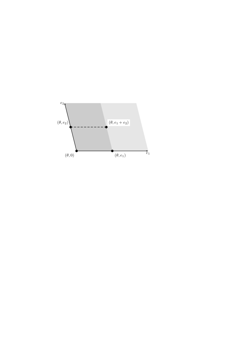
4.1 $\boldsymbol{\mathbbm{T}^{2}/\mathbbm{Z}_{2}}$ as a ‘product’ of two $\boldsymbol{\mathbbm{S}^{1}/\mathbbm{Z}_{2}}$ orbifolds

4.1.1 Generic situation

The $\mathbbm{T}^{2}/\mathbbm{Z}_{2}$ orbifold is obtained by dividing the torus by the reflection at the origin. The 2D torus is defined by a 2D lattice which is spanned by $e_{i}$ $(i=1,2)$. The $\mathbbm{Z}_{2}$ twist $\theta$ acts then on the $e_{i}$ as

$$\theta\,e_{i}~{}=~{}-e_{i}\;.$$ (52)

There are four fixed fixed points $(\theta,m_{1}\,e_{1}+m_{2}\,e_{2})$ where $m_{i}=0,1$ (figure 3).

Figure 3: $\mathbbm{T}^{2}/\mathbbm{Z}_{2}$. Points which are related by a reflection at the origin are identified. The fundamental region of the orbifold (dark gray region) is half of the fundamental region of the torus (gray region). By folding it along the dashed line and identifying the edges one obtains a ‘ravioli’ (or ‘pillow’) with the fixed points being the corners.

From the space group rule (7) one infers that a coupling involving $n$ localized states $|(\theta,m^{(j)}_{1}e_{1}+m^{(j)}_{2}e_{2}),\dots\rangle$ can be allowed only if

$$n \text{even}\;,$$ is

$$\sum_{j=1}^{n}m_{i}^{(j)} \text{even}\;,\quad i=1,2\;.$$ is (53)

As before, the selection rules can be rewritten in a different way. In a basis where the localized states appear as $\boldsymbol{4}$-plets, $|\boldsymbol{4}\rangle=\left(|(\theta,0),\dots\rangle,|(\theta,e_{1}),\dots\rangle,|(\theta,e_{2}),\dots\rangle,|(\theta,e_{1}+e_{2}),\dots\rangle\right)$, the selection rules (53) allow couplings only if they are invariant under $|\boldsymbol{4}\rangle\to A\,|\boldsymbol{4}\rangle$ with

$$A~{}\in~{}\{P,Q,R\}~{}=~{}\left\{\left(\begin{array}[]{cc}\sigma_{3}&0\\ 0&\sigma_{3}\end{array}\right),\,\left(\begin{array}[]{cc}\mathbbm{1}_{2}&0\\ 0&-\mathbbm{1}_{2}\end{array}\right),\,\left(\begin{array}[]{cc}-\mathbbm{1}_{2}&0\\ 0&-\mathbbm{1}_{2}\end{array}\right)\right\}\;.$$ (54)

Again, in the absence of Wilson lines, the fixed points are equivalent. Hence the Lagrangean is invariant under relabeling

$$m_{i}~{}\to~{}m_{i}+1\mod 2\;,\quad i=1,2\;.$$ (55)

This relabeling corresponds, as before, to a permutation symmetry. Here, we have two separate permutations that can be represented as $|\boldsymbol{4}\rangle\to S\,|\boldsymbol{4}\rangle$ and $|\boldsymbol{4}\rangle\to S^{\prime}\,|\boldsymbol{4}\rangle$ where

$$S~{}=~{}\left(\begin{array}[]{cc}\sigma_{1}&0\\ 0&\sigma_{1}\end{array}\right)\;,\quad S^{\prime}~{}=~{}\left(\begin{array}[]{cc}0&\mathbbm{1}_{2}\\ \mathbbm{1}_{2}&0\end{array}\right)$$ (56)

in the above basis.

The connection between the generators $\{\sigma_{1},\,\sigma_{3}\}$ of the flavor symmetry for $\mathbbm{S}^{1}/\mathbbm{Z}_{2}$ and that for $\mathbbm{T}^{2}/\mathbbm{Z}_{2}$ can be seen from

$$Q =~{}\sigma_{3}\otimes\mathbbm{1}_{2\times 2}\;, S^{\prime} =~{}\sigma_{1}\otimes\mathbbm{1}_{2\times 2}\;,$$

$$P =~{}\mathbbm{1}_{2\times 2}\otimes\sigma_{3}\;, S =~{}\mathbbm{1}_{2\times 2}\otimes\sigma_{1}\;,$$ (57)

where $\otimes$ denotes the Kronecker product. This construction can easily be generalized to other higher-dimensional orbifolds.

The non-Abelian symmetry group arising from $\mathbbm{T}^{2}/\mathbbm{Z}_{2}$ is hence comprised of the multiplicative closure of the above matrices $P$, $Q$, $R$, $S$ and $S^{\prime}$. We obtain a flavor symmetry $(S_{2}\times S_{2})\ltimes(\mathbbm{Z}_{2}\times\mathbbm{Z}_{2}\times\mathbbm{Z}_{2})$. This symmetry group has 32 elements, and is a subgroup of $D_{4}\times D_{4}$ which has 64 elements. It is very similar to the Dirac group (see, e.g., [28]). The reason for having less symmetry than what one would have for the product space $(\mathbbm{S}^{1}/\mathbbm{Z}_{2})\times(\mathbbm{S}^{1}/\mathbbm{Z}_{2})$ (i.e. $D_{4}\times D_{4}$) is that in $\mathbbm{T}^{2}/\mathbbm{Z}_{2}$ the automorphism $\theta$ reflects both $e_{i}$ simultaneously. Therefore one has a $\mathbbm{Z}_{2}$ less, and correspondingly half as many elements, as it should be. Because both $D_{4}$ factors have a common (‘diagonal’) $\mathbbm{Z}_{2}$, we call the flavor symmetry group $(D_{4}\times D_{4})/\mathbbm{Z}_{2}$. Note that the ‘would-be’ $(\boldsymbol{2},\boldsymbol{2})$ under $D_{4}\times D_{4}$ transforms as an irreducible $\boldsymbol{4}$-dimensional representation under $(D_{4}\times D_{4})/\mathbbm{Z}_{2}$.

4.1.2 Symmetry enhancement

An interesting situation arises when the torus $\mathbbm{T}^{2}$ has special symmetries. Consider the case where $e_{1}$ and $e_{2}$ have the same length, and enclose an angle of $120^{\circ}$. Then the symmetry gets enhanced since the distances between all orbifold fixed points coincide. One may now envisage the orbifold as a regular tetrahedron (figure 4) with the corners corresponding to the fixed points [15] (this observation has been recently revisited [31]).

(a) $\mathbbm{T}^{2}_{\mathrm{SU}(3)}/\mathbbm{Z}_{2}\,.$

(b) Tetrahedron.

Figure 4: If the $\mathbbm{T}^{2}$ lattice vectors have equal length and enclose $120^{\circ}$, one can also fold the fundamental region of $\mathbbm{T}^{2}/\mathbbm{Z}_{2}$ to a tetrahedron.

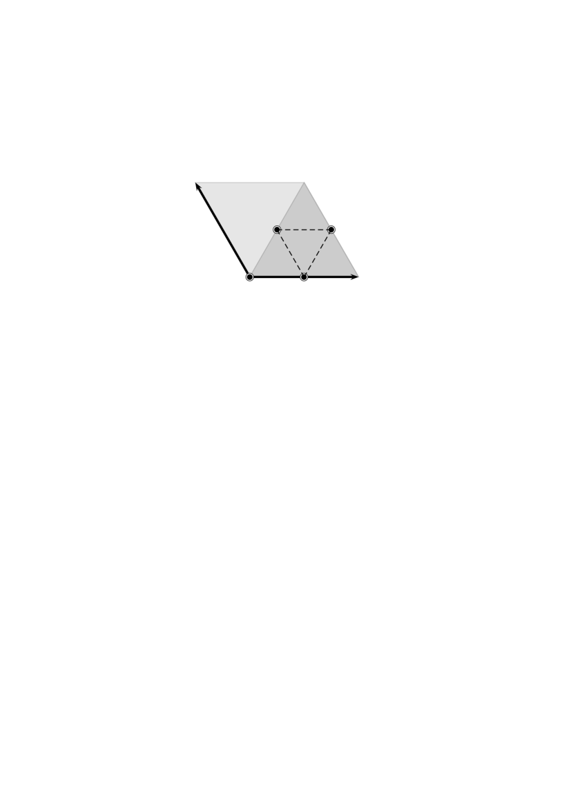
Clearly, the tetrahedron is invariant under a discrete rotation by $120^{\circ}$ about an axis that goes through one corner and hits the opposite surface orthogonally. This operation is represented by

$$T~{}=~{}\left(\begin{array}[]{cccc}1&0&0&0\\ 0&0&1&0\\ 0&0&0&1\\ 0&1&0&0\end{array}\right)\;,\quad T\,S\;,\quad T\,S^{\prime}\;,\quad T\,S\,S^{\prime}\;.$$ (62)

The full relabeling symmetry includes the symmetry of the tetrahedron, i.e. $A_{4}$. $A_{4}$ arises as multiplicative closure of the $\mathbbm{Z}_{2}$ and $\mathbbm{Z}_{3}$ groups with elements $\{\mathbbm{1},S\}$ and $\{\mathbbm{1},T,T^{2}\}$, respectively.

However, $A_{4}$ is not the full relabeling symmetry because the geometric relations between the fixed points do not change upon reflections (which, however, change the orientation, and are therefore not symmetries of the solid). The full relabeling symmetry is therefore $S_{4}$. As before, the flavor symmetry group is to be amended by the symmetries arising from the space group rules, i.e. one has to include the elements $P$, $Q$ and $R$. The flavor symmetry gets therefore enhanced to $S_{4}\ltimes(\mathbbm{Z}_{2}\times\mathbbm{Z}_{2}\times\mathbbm{Z}_{2})$, which is known as SW₄ in the literature [32], and has $4!\cdot 2^{3}=192$ elements. As before, the symmetry of the Lagrangean is larger than the symmetry of internal space. Recently an $A_{4}$ subgroup of the tetrahedral compactification symmetry SW₄ has been considered in the framework of neutrino mixing matrices in [31].

Another interesting case with enhanced symmetries is if (i) $e_{1}$ and $e_{2}$ enclose an angle of $90^{\circ}$ and (ii) $e_{1}$ and $e_{2}$ have equal length. The orbifold can then be envisaged as a perfect square with a fore- and a backside. One now has a relabeling symmetry consisting of cyclic permutations ($\mathbbm{Z}_{4}$), generated by

$$S^{\prime\prime}~{}=~{}\left(\begin{array}[]{cccc}0&1&0&0\\ 0&0&1&0\\ 0&0&0&1\\ 1&0&0&0\end{array}\right)\;,$$ (63)

plus the flips generated by $S$ and $S^{\prime}$. The multiplicative closure of the operations represented by $P$, $Q$, $R$, $S$, $S^{\prime}$ and $S^{\prime\prime}$ is $D_{4}\ltimes(\mathbbm{Z}_{2})^{3}$, and has 64 elements. It has 16 conjugacy classes, two four-dimensional, six two-dimensional and eight one-dimensional irreducible representations. From the construction, it is obvious that this order 64 group is a subgroup of the above-mentioned SW₄. Clearly, it contains the order 32 symmetry of the generic $\mathbbm{T}^{2}/\mathbbm{Z}_{2}$ as a subgroup.

An important remark, applicable to both cases above, concerns the symmetry breakdown occurring when the angle between $e_{1}$ and $e_{2}$ and/or their length ratio changes. Both the angle and the ratio are parametrized by a field $Z$, called complex structure modulus in the literature. Hence symmetry breakdown can be described by a departure of the vacuum expectation value (VEV) of $Z$ from its symmetric value. That is, the couplings between localized states are $Z$-dependent, and the coupling strengths respect an enhanced symmetry if $Z$ takes special values.

4.2 Other combinations of building blocks

From the above discussion it is clear how to obtain the flavor symmetries of other combinations of building blocks. In general, these emerge as products of the flavor symmetries of the building blocks with a common (‘diagonal’) $\mathbbm{Z}_{n}$ sub-group identified. As an example consider $\mathbbm{T}^{4}/\mathbbm{Z}_{2}$ where the flavor symmetry is $(D_{4}\times D_{4}\times D_{4}\times D_{4})/(\mathbbm{Z}_{2})^{3}=(S_{2}\times S_{2}\times S_{2}\times S_{2})\ltimes(\mathbbm{Z}_{2}^{5})$.

Exceptions to this statement occur if independent twists act on the building blocks. An example for such a situation is the $\mathbbm{Z}_{6}-\mathrm{II}=\mathbbm{Z}_{3}\times\mathbbm{Z}_{2}$ orbifold which enjoys a $\Delta(54)\times(D_{4}\times D_{4})/\mathbbm{Z}_{2}$ symmetry coming from the building blocks $\mathbbm{T}^{2}/\mathbbm{Z}_{3}$ and $\mathbbm{T}^{2}/\mathbbm{Z}_{2}$.

We note that such large flavor symmetry groups would not be expected in realistic models because they only arise in the absence of Wilson lines, where one often obtains too many families. Moreover, Wilson lines are generically needed in order to reduce the gauge symmetry to the standard model gauge group (amended by a ‘hidden sector’).

orbifold	flavor symmetry	twisted sector	string fundamental states
$\mathbbm{S}^{1}/\mathbbm{Z}_{2}$	$D_{4}$ $=S_{2}\ltimes(\mathbbm{Z}_{2}\times\mathbbm{Z}_{2})$	untwisted sector	$\boldsymbol{1}$
		$\theta$-twisted sector	2
$\mathbbm{T}^{2}/\mathbbm{Z}_{2}$	$(D_{4}\times D_{4})/\mathbbm{Z}_{2}$ $=(S_{2}\times S_{2})\ltimes\mathbbm{Z}_{2}^{3}$	untwisted sector	$\boldsymbol{1}$
		$\theta$-twisted sector	$\boldsymbol{4}$
$\mathbbm{T}^{2}/\mathbbm{Z}_{3}$		untwisted sector	$\boldsymbol{1}$
	$\Delta(54)$ $=S_{3}\ltimes(\mathbbm{Z}_{3}\times\mathbbm{Z}_{3})$	$\theta$-twisted sector	3
		$\theta^{2}$-twisted sector	${\bar{\bf 3}}$
$\mathbbm{T}^{2}/\mathbbm{Z}_{4}$		untwisted sector	$\boldsymbol{1}$
	$(D_{4}\times\mathbbm{Z}_{4})/\mathbbm{Z}_{2}$	$\theta$-twisted sector	2
		$\theta^{2}$-twisted sector	$\boldsymbol{1}_{A_{1}}+\boldsymbol{1}_{B_{1}}+\boldsymbol{1}_{B_{2}}+\boldsymbol{1}_{A_{2}}$
$\mathbbm{T}^{2}/\mathbbm{Z}_{6}$	trivial
$\mathbbm{T}^{4}/\mathbbm{Z}_{8}$		untwisted sector	$\boldsymbol{1}$
		$\theta$-twisted sector	2
	$(D_{4}\times\mathbbm{Z}_{8})/\mathbbm{Z}_{2}$	$\theta^{2}$-twisted sector	$\boldsymbol{1}_{A_{1}}+\boldsymbol{1}_{B_{1}}+\boldsymbol{1}_{B_{2}}+\boldsymbol{1}_{A_{2}}$
		$\theta^{3}$-twisted sector	2
		$\theta^{4}$-twisted sector	$4\times(\boldsymbol{1}_{A_{1}}+\boldsymbol{1}_{B_{1}}+\boldsymbol{1}_{B_{2}}+\boldsymbol{1}_{A_{2}})$
$\mathbbm{T}^{4}/\mathbbm{Z}_{12}$	trivial
$\mathbbm{T}^{6}/\mathbbm{Z}_{7}$		untwisted sector	$\boldsymbol{1}$
	$S_{7}\ltimes(\mathbbm{Z}_{7})^{6}$	$\theta^{k}$-twisted sector	$\boldsymbol{7}$
		$\theta^{7-k}$-twisted sector	${\bar{\bf 7}}$

Table 2: Non-Abelian discrete flavor symmetries of the building blocks.

It is also clear that symmetry enhancement occurs in various orbifolds. In table 1 (a), there are three more cases where the flavor symmetry can be enlarged: $\mathbbm{T}^{4}/\mathbbm{Z}_{4}$, $\mathbbm{T}^{4}/\mathbbm{Z}_{3}$, $\mathbbm{T}^{6}/\mathbbm{Z}_{3}$. A similar analysis as above shows that for the $\mathbbm{T}^{4}/\mathbbm{Z}_{4}$ orbifold, in the case that an $S_{4}$ permutation symmetry is realized between the states at the four fixed points of the four dimensional sublattice, the full flavor symmetry will again be SW₄.

For the generic case of the $\mathbbm{T}^{4}/\mathbbm{Z}_{3}$ orbifold we find a flavor symmetry group $(S_{3}\times S_{3})\ltimes(\mathbbm{Z}_{3})^{3}$. If the geometric set-up allows an enlargement of the relabeling symmetry from $S_{3}\times S_{3}$ to $S_{9}$, this group becomes even larger and can be written as $S_{9}\ltimes(\mathbbm{Z}_{3})^{8}$. Similarly, for $\mathbbm{T}^{6}/\mathbbm{Z}_{3}$, the flavor symmetry could be enhanced to include the permutation symmetry $S_{27}$.

We can also study discrete non-Abelian flavor symmetries at enhancement points in 6D $\mathbbm{Z}_{N}\times\mathbbm{Z}_{M}$ orbifold models. Certain classes of $\mathbbm{Z}_{N}\times\mathbbm{Z}_{M}$ orbifold models at such enhancement points [33] are equivalent to Gepner models [34]. Therefore, our analysis is available to such types of Gepner models.

5 Comments on symmetry breaking

An important question concerns the symmetry breaking patterns of the above flavor symmetries. As mentioned, the symmetries are explicitly broken by the introduction of non-trivial discrete Wilson lines. That is, in this case the degeneracies of mass spectra on different fixed points are lifted, and no non-Abelian subgroups remain.

On the other hand, when one scalar field in a multiplet of a non-Abelian symmetry acquires a VEV, a non-Abelian subgroup remains unbroken. Let us consider, for example, the 2D $\mathbbm{T}^{2}/\mathbbm{Z}_{3}$ orbifold. It has $\Delta(54)=S_{3}\ltimes(\mathbbm{Z}_{3}\times\mathbbm{Z}_{3})$ flavor structure, and degenerate matter fields at three independent fixed points correspond to a triplet. Suppose that a scalar field at one of the fixed points, e.g. $(\theta,0)$, develops a VEV. In this case, $S_{3}$ of $S_{3}\ltimes(\mathbbm{Z}_{3}\times\mathbbm{Z}_{3})$ is broken as $S_{3}\rightarrow S_{2}$, and $(\mathbbm{Z}_{3}\times\mathbbm{Z}_{3})$ is broken as $\mathbbm{Z}_{3}\times\mathbbm{Z}_{3}\rightarrow\mathbbm{Z}_{3}$. Hence, the remaining flavor symmetry is the $D_{3}=S_{2}\ltimes\mathbbm{Z}_{3}$ symmetry, which consists of the 6 elements

$$\left(\begin{array}[]{cc}1&0\\ 0&1\end{array}\right),\quad\left(\begin{array}[]{cc}0&1\\ 1&0\end{array}\right),\quad\left(\begin{array}[]{cc}\omega&0\\ 0&\omega^{2}\end{array}\right),\quad\left(\begin{array}[]{cc}\omega^{2}&0\\ 0&\omega\end{array}\right),\quad\left(\begin{array}[]{cc}0&\omega\\ \omega^{2}&0\end{array}\right),\quad\left(\begin{array}[]{cc}0&\omega^{2}\\ \omega&0\end{array}\right)\;.$$ (64)

Here, the $\theta$-twisted states $|(\theta,e_{1})\rangle$ and $|(\theta,2e_{1})\rangle$ correspond to a $D_{3}$-doublet. The $D_{3}$ symmetry is the only non-Abelian group obtained from $\Delta(54)$ by a VEV of the ${\bf 3}$ as shown in appendix C. Recall that only triplets as well as trivial singlets appear as string fundamental states. However, products of triplets include other non-trivial representations. If condensates of such modes form, this could give rise to other breaking patterns. In appendix C, all subgroups of $\Delta(54)$ are shown.

Similarly, we can study breaking patterns of the flavor symmetry $S_{7}\ltimes(\mathbbm{Z}_{7})^{6}$, which appears in $\mathbbm{Z}_{7}$ orbifold models. A similar type of breaking would lead to the flavor symmetry, $S_{n}\ltimes(\mathbbm{Z}_{7})^{n-1}$ with $n<7$.

Let us now comment on how frequent non-Abelian discrete flavor symmetries arise in realistic orbifold models. The most obvious possibility to accommodate the observed repetition of families is to construct a model where some or all families stem from equivalent fixed points. As we have seen, this leads to a permutation symmetry which, when combined with the other (stringy) symmetries, gives rise to a non-Abelian flavor symmetry. This symmetry is exact at the orbifold point, where the expectation values of all (charged) zero modes vanish. However, the orbifold point is, in general, not a valid vacuum of the model because of Fayet-Iliopoulos $D$-term. Cancellation of the $D$-term requires certain fields (which have to be SM singlets for the model to be realistic) to acquire VEVs. These VEVs lead generically to a spontaneous breakdown of the non-Abelian discrete flavor symmetries. Another common feature of realistic orbifold models seems to be the existence of vector-like pairs of SM representations and anti-representations (cf. [19, 20]). The SM families mix with these states so that the chiral states observed at low energies are linear combinations of the states transforming under the non-Abelian discrete flavor symmetries with flavor singlets (while orthogonal linear combinations of vector-like matter get large masses). This mixing might be important in order to reproduce the observed flavor pattern [35, 20]. Altogether, we expect non-Abelian discrete flavor symmetries to be generic to realistic orbifold models. These symmetries are usually spontaneously broken in the vacuum, and the pattern of observed Yukawa couplings is also affected by the mixing of the chiral SM representations with vector-like states.

We also expect these symmetries to play an important role in understanding the structure of soft supersymmetry breaking terms. For example, degeneracy due to non-Abelian flavor symmetry would be useful to suppress dangerous flavor changing neutral currents (see, e.g., [36, 21]). It appears possible to arrive at a situation where in the Kähler potential, and therefore in the soft terms, the non-Abelian discrete symmetries survive while the Yukawa couplings receive important modifications from spontaneous symmetry breakdown.

6 Conclusions and discussion

We have studied the origin of non-Abelian discrete flavor symmetries in string theory. We have classified all the possible non-Abelian discrete flavor symmetries which can appear in heterotic orbifold models. We find that these symmetries exist in many orbifolds, and have a very simple geometric interpretation. In particular, they are always present in constructions where the repetition of SM families is explained by the multiplicity of equivalent fixed points. A crucial ingredient is the permutation symmetry of such equivalent fixed points which, together with other symmetries from the space-group selection rule, generates non-Abelian flavor symmetries such as $D_{4}$ and $\Delta(54)$, as well as their direct products. A key property of the flavor symmetry is that it is always larger than the geometrical symmetry of the compact space. We have also seen that the flavor symmetries can get enhanced if the internal space respects certain symmetries beyond the orbifold twist. We have further discussed how flavor symmetries can be broken to smaller non-Abelian flavor symmetries such as $D_{3}$. At this point, we would like to remind the reader that the symmetry emerging from the space group is to be amended by symmetries coming from gauge invariance and $H$-momentum conservation. That is, there are in general additional gauge factors (e.g. U(1) factors) and discrete $R$-symmetries restricting the couplings. Besides, from non-Abelian gauge factors one may, in principle, obtain further non-Abelian discrete symmetries which have not been discussed here.

It should be interesting to repeat our analysis in non-factorizable orbifolds, which were recently constructed [37]. Furthermore, our analysis could be extended to string models with other types of backgrounds, e.g. Gepner manifolds and more general Calabi-Yau manifolds. For example, some of the Gepner models are equivalent to certain classes of orbifold models at enhancement points of moduli spaces. On the other hand, blowing-up orbifold singularities would lead to certain classes of Calabi-Yau manifolds, and such procedure corresponds to a spontaneous breakdown of (non-Abelian) discrete flavor symmetries, as discussed before.

In this paper, we have focused on the derivation and classification of non-Abelian discrete symmetries. It should be interesting to study phenomenological applications of our results, such as the understanding of the observed Yukawa matrices of quarks and leptons in terms of spontaneously broken flavor symmetries, taking into account the mixing with vector-like states. The identification of phenomenologically successful flavor symmetries might lead to the identification of geometries which are particularly useful for obtaining realistic string compactifications.

Acknowledgments

It is a pleasure to thank C. Hagedorn and P.K.S. Vaudrevange for useful discussions. T. K. would like to thank Physikalisches Institut, Universität Bonn for hospitality during his stay. T. K. is supported in part by the Grand-in-Aid for Scientific Research #17540251 and the Grant-in-Aid for the 21st Century COE “The Center for Diversity and Universality in Physics” from the Ministry of Education, Culture, Sports, Science and Technology of Japan. This work was partially supported by the European Union 6th Framework Program MRTN-CT-2004-503369 “Quest for Unification” and MRTN-CT-2004-005104 “ForcesUniverse”. S. R. received partial support from DOE grant DOE/ER/01545-869, and would like to thank the Kavli Institute for Theoretical Physics, Santa Barbara, CA for their hospitality while this paper was being finished. This research was supported in part by the National Science Foundation under Grant No. PHY99-07949.

Appendix A Couplings on orbifolds

In this appendix we outline the calculation of coupling strengths on orbifolds. Let us start with trilinear couplings. Yukawa couplings are obtained by calculating 3-point functions including three vertex operators corresponding to massless modes. In heterotic orbifold models, vertex operators consist of a 4D space-time part, a 6D orbifold part, a gauge part and a bosonized fermion part. The vertex operators for the 6D orbifold part, the so-called twist fields, are relevant to our study on flavor symmetries. One twist field $\sigma_{(\theta^{k},\ell)}(z)$ is assigned to each mode on the fixed point $(\theta^{k},\ell)$, that is, each massless mode corresponding to the boundary condition $(\theta^{k},\ell)$. Thus, Yukawa couplings corresponding to three fields on fixed points $(\theta^{k^{(j)}},\ell^{(j)})$ $(j=1,2,3)$ are obtained through the calculation of $\langle\sigma_{(\theta^{k^{(1)}},\ell^{(1)})}\sigma_{(\theta^{k^{(2)}},\ell^{(2)})}\sigma_{(\theta^{k^{(3)}},\ell^{(3)})}\rangle$. It can be decomposed as the sum of classical solutions and quantum fluctuations around them, that is,

$$\left\langle\sigma_{(\theta^{k^{(1)}},\ell^{(1)})}\sigma_{(\theta^{k^{(2)}},\ell^{(2)})}\sigma_{(\theta^{k^{(3)}},\ell^{(3)})}\right\rangle~{}=~{}Z_{\mathrm{qu}}\sum_{X_{\mathrm{cl}}}\,e^{-S_{\mathrm{cl}}}\;,$$ (65)

where $Z_{\mathrm{qu}}$ is the quantum part, $X_{\mathrm{cl}}$ denotes classical solutions and $S_{\mathrm{cl}}$ is its classical action. The quantum part $Z_{\mathrm{qu}}$ is independent of locations of fixed points, but locations of fixed points are relevant to $S_{\mathrm{cl}}$. The classical solution (world-sheet instanton) is obtained as

$$\partial Z^{i}_{\mathrm{cl}}~{}=~{}a^{i}\,(z-z_{1})^{-1+k^{(1)}v^{(1),i}}\,(z-z_{2})^{-1+k^{(2)}v^{(2),i}}\,(z-z_{3})^{-1+k^{(3)}v^{(3),i}}\;,$$ (66)

where $Z^{i}=X^{2i-1}+X^{2i}$ and $z_{i}$ is the inserted point of $i$-th vertex operator $\sigma_{(\theta^{k^{(j)}},\ell^{(j)})}$ on the complex coordinate of the string world-sheet. The constants $a^{i}$ are determined by the global monodromy condition, e.g. for the contour around $z_{1}$ and $z_{2}$ as

$$a^{i}~{}=~{}C(k^{(1)}v^{(1),i},k^{(2)}v^{(2),i})(f^{(1),i}-f^{(2),i})\;,$$ (67)

where $C(k^{(1)}v^{(1),i},k^{(2)}v^{(2),i})$ is a constant depending only on $k^{(1)}v^{(1),i}$ and $k_{(2)}v^{(2),i}$ and $f^{(a),i}$ denotes the fixed point corresponding to $\sigma_{(\theta^{k^{(a)}},\ell^{(a)})}$ in the complex basis $Z^{i}$. We substitute this solution into the action,

$$S_{\mathrm{cl}}~{}=~{}\frac{1}{4\pi\alpha^{\prime}}\int\mathrm{d}^{2}z\,(\partial Z_{\mathrm{cl}}\bar{\partial}\bar{Z}_{\mathrm{cl}}+\bar{\partial}Z_{\mathrm{cl}}\partial\bar{Z}_{\mathrm{cl}})\;,$$ (68)

then we can calculate the classical action. Here we take the solution $\bar{\partial}Z_{\mathrm{cl}}=0$. Otherwise, the action does not become finite and does not contribute to the above amplitude. As a result, the magnitude of Yukawa coupling is obtained as

$$Y~{}\sim~{}e^{-A},$$ (69)

where $A$ is the area which the string sweeps to couple. This result is the same when we use another contour for the global monodromy condition, e.g. the contour around $z_{2}$ and $z_{3}$. Note that the fixed point $(\theta^{k_{(a)}},\ell_{(a)})$ is equivalent to $(\theta^{k_{(a)}},\ell_{(a)}+(1-\theta^{k_{(a)}})\Lambda)$. Thus, we have to sum over classical solutions belonging to the same conjugacy classes, although the classical solution corresponding to the shortest distance is dominant and the others lead to larger classical actions and subdominant effects.

Similarly one can estimate magnitudes of generic $n$-point couplings [38]. As before, the $n$-point function decomposes into a quantum part and a classical part. Classical solutions have more variety and become complicated. For example, solutions with $\bar{\partial}Z\neq 0$ also lead to any rate, the classical actions only depend on distances between fixed points $f^{(a)}-f^{(b)}$ as well as angles between distance vectors, $f^{(a)}-f^{(b)}$ and $f^{(c)}-f^{(d)}$.

Appendix B $\boldsymbol{D_{4}}$ symmetry

The $D_{4}$ discrete group has five representations including a doublet $D$, a trivial singlet $A_{1}$ and three non-trivial singlets $B_{1},B_{2},A_{2}$. Table 3 lists the characters of these five representations.

Representations	$\mathbbm{1}$	$-\mathbbm{1}$	$\pm\sigma_{1}$	$\pm\sigma_{3}$	$\mp\mathrm{i}\sigma_{2}$
Doublet$-D$	2	–2	0	0	0
Singlet$-A_{1}$	1	1	1	1	1
Singlet$-B_{1}$	1	1	1	–1	–1
Singlet$-B_{2}$	1	1	–1	1	–1
Singlet$-A_{2}$	1	1	–1	–1	1

Table 3: Character table for $D_{4}$.

A product of two doublets decomposes into four singlets,

$$(D\times D)~{}=~{}A_{1}+B_{1}+B_{2}+A_{2}\;.$$ (70)

More explicitly, we consider two $D_{4}$ doublets $S_{A}$ and $\bar{S}_{A}$ $(A=1,2)$. Their product $S_{A}\bar{S}_{B}$ can be decomposed in terms of $A_{1},B_{1},B_{2},A_{2}$,

$$S_{1}\bar{S}_{1}+S_{2}\bar{S}_{2} \sim~{}A_{1}\;, S_{1}\bar{S}_{2}+S_{2}\bar{S}_{1} \sim~{}B_{1}\;,$$

$$S_{1}\bar{S}_{1}-S_{2}\bar{S}_{2} \sim~{}B_{2}\;, S_{1}\bar{S}_{2}-S_{2}\bar{S}_{1} \sim~{}A_{2}\;.$$ (71)

Appendix C $\boldsymbol{\Delta(54)}$ symmetry

Group-theoretical aspects of $\Delta(54)$ can be found in [30, 41]. It is a discrete subgroup of $\mathrm{SU}(3)$, i.e. the group $\Delta(6n^{2})$ (with $n=3$) and order $54\,(=3!\cdot 3^{2})$. The generators of $\Delta(54)$ are given by the set

$$\left(\begin{array}[]{ccc}0&1&0\\ 0&0&1\\ 1&0&0\end{array}\right)\;,\quad\left(\begin{array}[]{ccc}e^{\mathrm{i}\,\alpha}&0&0\\ 0&e^{\mathrm{i}\,\beta}&0\\ 0&0&e^{-\mathrm{i}\,(\alpha+\beta)}\end{array}\right)\;,\quad\left(\begin{array}[]{ccc}e^{\mathrm{i}\,\alpha}&0&0\\ 0&0&e^{\mathrm{i}\,\beta}\\ 0&e^{-\mathrm{i}\,(\alpha+\beta)}&0\end{array}\right)\;,$$ (72)

with $\alpha=2\pi j/3$, $\beta=2\pi k/3$ and $j,k$ integers. In general, it has four three dimensional irreducible representations $\mathbf{3},\,\mathbf{\bar{3}},\,\mathbf{3^{\prime}},\,\mathbf{\bar{3^{\prime}}}\,$, four two dimensional ones $\mathbf{2}_{1},\,\mathbf{2}_{2},\,\mathbf{2}_{3},\,\mathbf{2}_{4}$ and two one dimensional ones $\mathbf{1}_{1},\,\mathbf{1}_{2}$. Their characters are summarized in table 4. The subgroups of $\Delta(54)$ are given in table 5.

irrep 1a 6a 6b 3a 3b 3c 2a 3d 3e 3f (1) (9) (9) (6) (6) (6) (9) (6) (1) (1) $\mathbf{1}_{1}$ 1 1 1 1 1 1 1 1 1 1 $\mathbf{1}_{2}$ 1 -1 -1 1 1 1 -1 1 1 1 $\mathbf{2}_{1}$ 2 0 0 2 -1 -1 0 -1 2 2 $\mathbf{2}_{2}$ 2 0 0 -1 -1 -1 0 2 2 2 $\mathbf{2}_{3}$ 2 0 0 -1 -1 2 0 -1 2 2 $\mathbf{2}_{4}$ 2 0 0 -1 2 -1 0 -1 2 2 $\mathbf{3^{\prime}}$ 3 $-\bar{\omega}$ $-\omega$ 0 0 0 -1 0 $3\bar{\omega}$ $3\omega$ $\mathbf{\bar{3^{\prime}}}$ 3 $-\omega$ $-\bar{\omega}$ 0 0 0 -1 0 $3\omega$ $3\bar{\omega}$ $\mathbf{\bar{3}}$ 3 $\omega$ $\bar{\omega}$ 0 0 0 1 0 $3\omega$ $3\bar{\omega}$ $\mathbf{3}$ 3 $\bar{\omega}$ $\omega$ 0 0 0 1 0 $3\bar{\omega}$ $3\omega$

Table 4: Character table of the group $\Delta(54)$ (with $\omega=e^{2\pi\mathrm{i}/3}$). The second row gives the number of elements in the certain class and the second column the dimension of the representation.

subgroup decomposition of $\boldsymbol{3}$ subgroup decomposition of $\boldsymbol{3}$ $\Delta(27)$ $\boldsymbol{3}$ $S_{3}$ $\boldsymbol{2}+\boldsymbol{1_{1}}$ $S_{3}\ltimes\mathbbm{Z}_{3}$ $\boldsymbol{2_{2}}+\boldsymbol{\overline{1_{4}}}$ $\mathbbm{Z}_{2}$ $2\cdot\boldsymbol{1_{1}}+\boldsymbol{1_{2}}$ $\mathbbm{Z}_{3}\times\mathbbm{Z}_{3}$ $\boldsymbol{\overline{1_{2}}}+\boldsymbol{\overline{1_{3}}}+\boldsymbol{1_{4}}$

Table 5: Decomposition of the $\boldsymbol{3}$ of $\Delta(54)$ into irreps of the particular subgroup under the breaking.

References

- [1] C. D. Froggatt and H. B. Nielsen, Nucl. Phys. B 147 (1979) 277.
- [2] P. H. Frampton and T. W. Kephart, Int. J. Mod. Phys. A 10 (1995) 4689 [arXiv:hep-ph/9409330].
-
[3]
S. Pakvasa and H. Sugawara,
Phys. Lett. B 73 (1978) 61;
L. J. Hall and H. Murayama, Phys. Rev. Lett. 75, 3985 (1995);
R. Dermisek and S. Raby, Phys. Rev. D 62, 015007 (2000). -
[4]
Phys. Lett. B 82 (1979) 105;
C. Hagedorn, M. Lindner and R. N. Mohapatra, arXiv:hep-ph/0602244. -
[5]
D. Wyler,
Phys. Rev. D 19 (1979) 3369;
E. Ma and G. Rajasekaran, Phys. Rev. D 64, 113012 (2001). - [6] W. Grimus and L. Lavoura, Phys. Lett. B572, 189 (2003).
- [7] C. Hagedorn, M. Lindner and F. Plentinger, arXiv:hep-ph/0604265.
- [8] K. S. Babu and J. Kubo, Phys. Rev. D 71, 056006 (2005).
- [9] D. B. Kaplan and M. Schmaltz, Phys. Rev. D 49, 3741 (1994).
- [10] K. C. Chou and Y. L. Wu, Phys. Rev. D 53, 3492 (1996).
- [11] I. de Medeiros Varzielas, S. F. King and G. G. Ross, arXiv:hep-ph/0607045.
- [12] L. J. Dixon, J. A. Harvey, C. Vafa and E. Witten, Nucl. Phys. B 261, 678 (1985); Nucl. Phys. B 274, 285 (1986).
[13]
L. E. Ibáñez, H.-P. Nilles and F. Quevedo, Phys. Lett. B 187, 25 (1987);
L. E. Ibáñez, J. E. Kim, H.-P. Nilles and F. Quevedo, Phys. Lett. B 191, 282 (1987);
L. E. Ibáñez, J. Mas, H. P. Nilles and F. Quevedo, Nucl. Phys. B 301, 157 (1988);
A. Font, L. E. Ibáñez, F. Quevedo and A. Sierra, Nucl. Phys. B 331, 421 (1990);
D. Bailin, A. Love and S. Thomas, Phys. Lett. B 194, 385 (1987). - [14] S. Hamidi and C. Vafa, Nucl. Phys. B 279, 465 (1987);
- [15] L. J. Dixon, D. Friedan, E. J. Martinec and S. H. Shenker, Nucl. Phys. B 282, 13 (1987).
[16]
T. Kobayashi and N. Ohtsubo,
Int. J. Mod. Phys. A 9, 87 (1994);
J. A. Casas, F. Gomez and C. Muñoz, Int. J. Mod. Phys. A 8, 455 (1993). - [17] T. Kobayashi, S. Raby and R. J. Zhang, Phys. Lett. B 593, 262 (2004).
- [18] T. Kobayashi, S. Raby and R. J. Zhang, Nucl. Phys. B 704, 3 (2005).
- [19] W. Buchmüller, K. Hamaguchi, O. Lebedev and M. Ratz, Phys. Rev. Lett. 96, 121602 (2006).
- [20] W. Buchmüller, K. Hamaguchi, O. Lebedev and M. Ratz, arXiv:hep-th/0606187.
- [21] P. Ko, T. Kobayashi, J.h. Park, S. Raby and R.J. Zhang, in preparation.
- [22] Y. Katsuki, Y. Kawamura, T. Kobayashi, N. Ohtsubo, Y. Ono and K. Tanioka, Nucl. Phys. B 341 (1990) 611.
- [23] S. Förste, H. P. Nilles, P. K. S. Vaudrevange and A. Wingerter, Phys. Rev. D 70, 106008 (2004).
- [24] A. Font, L. E. Ibáñez and F. Quevedo, Phys. Lett. B 217, 272 (1989).
[25]
T. T. Burwick, R. K. Kaiser and H. F. Müller,
Nucl. Phys. B 355, 689 (1991);
J. Erler, D. Jungnickel, M. Spalinski and S. Stieberger, Nucl. Phys. B 397, 379 (1993). - [26] W. Buchmüller, K. Hamaguchi, O. Lebedev and M. Ratz, Nucl. Phys. B 712, 139 (2005).
- [27] M. Hall, “The Theory of Groups”, Chelsea, New York (1976).
- [28] J. S. Lomont, “Applications of Finite Groups”, New York: Dover (1987).
- [29] C. W. Curtis and I. Reiner,“Representation Theory of Finite Groups and Associative Algebras”, New York: Wiley-Interscience (1962).
- [30] W. M. Fairbairn, T. Fulton and W. H. Klink, J. of Math. Phys. 5, 1038 (1964).
- [31] G. Altarelli, F. Feruglio and Y. Lin, arXiv:hep-ph/0610165.
- [32] M. Baake, B. Gemünden and R. Oedingen, J. Math. Phys. 23 (1982) 944 [Erratum-ibid. 23 (1982) 2595].
[33]
E. J. Chun and J. E. Kim,
Phys. Lett. B 238, 265 (1990);
E. J. Chun, J. Lauer and H. P. Nilles, Int. J. Mod. Phys. A 7, 2175 (1992);
T. Kobayashi, N. Ohtsubo and K. Tanioka, Int. J. Mod. Phys. A 8, 3553 (1993);
H. Kawabe, T. Kobayashi and N. Ohtsubo, Prog. Theor. Phys. 88, 431 (1992). - [34] D. Gepner, Phys. Lett. B 199, 380 (1987); Nucl. Phys. B 296, 757 (1988).
- [35] T. Asaka, W. Buchmüller and L. Covi, Phys. Lett. B 563 (2003) 209 [arXiv:hep-ph/0304142].
- [36] O. Lebedev, arXiv:hep-ph/0506052.
- [37] A. E. Faraggi, S. Förste and C. Timirgaziu, arXiv:hep-th/0605117.
- [38] K. S. Choi and T. Kobayashi, in progress.
- [39] S. A. Abel and A. W. Owen, Nucl. Phys. B 682, 183 (2004).
- [40] H. Georgi, “Lie Algebras In Particle Physics. From Isospin To Unified Theories”, Front. Phys. 54 (1982) 1.
- [41] T. Muto, JHEP 9902, 008 (1999) [arXiv:hep-th/9811258].