Phenomenology of the Left-Right Twin Higgs Model

Abstract

The twin Higgs mechanism has recently been proposed to solve the little hierarchy problem. We study the implementation of the twin Higgs mechanism in left-right models. At TeV scale, heavy quark and gauge bosons appear, with rich collider phenomenology. In addition, there are extra Higgses, some of which couple to both the Standard Model fermion sector and the gauge sector, while others couple to the gauge bosons only. We present the particle spectrum, and study the general features of the collider phenomenology of this class of model at the Large Hadron Collider.

I Introduction

The Higgs mechanism provides a simple and elegant method to explain the electroweak symmetry breaking in the Standard Model (SM). The Higgs boson, however, is yet to be found. While we do not know whether the Higgs boson exists, unitarity indicates that new physics is very likely to be found at the large hadron collider (LHC) LeeEG .

If the electroweak symmetry is broken by the Higgs mechanism, the current lower limit on the mass of a scalar SM Higgs comes from LEP Higgs searches: $m_{h}>114$ GeV LEPHiggs . Electroweak precision measurements from LEP and SLC set an upper bound on the Higgs mass: $m_{h}<219$ GeV at 95% C.L. mhlimit . The leading quadratically divergent radiative corrections to the Higgs mass require the scale of new physics to be around TeV scale. Otherwise, fine tuning in the Higgs potential becomes severe. On the other hand, precision measurements constrain the cutoff scale for new physics to be likely above 5$-$10 TeV , leading to a few percent fine tuning in the Higgs potential. This is the so called little hierarchy problem or the LEP paradox LEPparadox .

Recently, the twin Higgs mechanism has been proposed as a solution to the little hierarchy problem twinhiggsmirror ; twinhiggsleftright ; susytwinhiggs . The Higgses emerge as pseudo-Goldstone bosons once the global symmetry is spontaneously broken. Gauge and Yukawa interactions that break the global symmetry give masses to the Higgses, with the leading order being quadratically divergent. When an additional discrete symmetry is imposed, the leading quadratically divergent terms respect the global symmetry. Thus they do not contribute to the Higgs masses. The resulting Higgs masses obtain logarithmically divergent contributions. The Higgs masses are around the electroweak scale when the cutoff is around 5$-$10 TeV.

The twin Higgs mechanism can be implemented in different ways. In the mirror twin Higgs models twinhiggsmirror , a complete copy of the SM is introduced, both the gauge interactions and the particle content. The discrete symmetry is identified with mirror parity. The leading SM contributions to the Higgs masses are canceled by the contributions from the mirror particles. The particles in the mirror world communicate with the SM particles only via the Higgs particles. For the mirror quarks and leptons, they are charged under the mirror gauge groups, not the SM ones. Therefore, those mirror particles can seldom be produced at colliders. The Higgs can decay invisibly into mirror bottom quark. The coupling between the SM Higgs and the mirror bottom quark is suppressed by $v/(\sqrt{2}f)$, comparing to the Standard Model $h\bar{b}b$ coupling. Here $v$ is the Higgs vacuum expectation value (vev) $v=246$ GeV and $f$ is the symmetry breaking scale in the mirror twin Higgs model, which is typically around 800 GeV. Numerically, the invisible Higgs decay branching ratio is about $5\%$. The searches for invisible Higgs decay at the LHC have been studied in the literature invisible ; zeppenfeld ; cmsWBF ; atlasWBF ; atlasZH ; atlasttH . Analyses in Ref. zeppenfeld show that for a Higgs mass of 120 GeV with SM production cross section, an invisible decay branching ratio of about 13% (5%) can be probed at 95% C.L. for an integrated luminosity of 10 (100) ${\rm fb}^{-1}$ at the LHC via weak boson fusion process. Following the strategy in Ref. zeppenfeld , more detailed analyses including detector simulation at ATLAS atlasWBF show that an invisible Higgs decay branching ratio of about 36% (25%) can be probed at 95% C.L. at the LHC with 10 (30) ${\rm fb}^{-1}$ integrated luminosity. More recent analyses cmsWBF show that CMS should be able to probe an invisible Higgs decay branching ratio as low as 12% with 10 ${\rm fb}^{-1}$. Results based on analyses with $Zh$, $Wh$ atlasZH or $t\bar{t}h$ atlasttH production channel are less competitive. Therefore, a measurement of $5\%$ invisible Higgs decay would be possible at the LHC.

The twin Higgs mechanism can also be implemented in left-right models with the discrete symmetry being identified with left-right symmetry twinhiggsleftright . In the left-right twin Higgs (LRTH) model, the global symmetry is ${\rm U}(4)\times{\rm U}(4)$, with a gauged ${\rm SU}(2)_{L}\times{\rm SU}(2)_{R}\times{\rm U}(1)_{B-L}$ subgroup. After Higgses obtain vacuum expectation values, the global symmetry ${\rm U}(4)\times{\rm U}(4)$ breaks down to ${\rm U}(3)\times{\rm U}(3)$, and ${\rm SU}(2)_{R}\times{\rm U}(1)_{B-L}$ breaks down to the SM ${\rm U}(1)_{Y}$. Three Goldstone bosons are eaten by the massive gauge bosons $Z_{H}$ and $W_{H}^{\pm}$, while the remaining Goldstone bosons contain the SM ${\rm SU}(2)_{L}$ Higgs doublet and extra Higgses. The leading quadratically divergent SM gauge boson contributions to the Higgs masses are canceled by the loop involving the heavy gauge bosons. A vector top singlet pair is introduced to generate an ${\cal O}(1)$ top Yukawa coupling. The quadratically divergent SM top contributions to the Higgs potential are canceled by the contributions from a heavy top partner. Many new particles which have order of one interaction strength with the SM sector are predicted and rich phenomenology is expected at the LHC.

This paper is organized as follows. Sec. II describes the LRTH model in detail. We present the particle content, and the structure of gauge and Yukawa interactions. After spontaneous symmetry breaking, we calculate the particle spectrum, and write down the resulting Feynman rules for the interactions. We demonstrate the twin Higgs mechanism in Sec. III. In Sec. IV, we show numerical values of the particle masses. In Sec. V, we summarize the current experimental constraints on the model parameters. In Sec. VI, we discuss in detail the collider phenomenology of the left-right twin Higgs model. We analyze the particle production cross sections, and their decay patterns. Sec. VII is devoted to the discussion of the case when the mass mixing between the extra vector top quark singlet is zero or very small ($\lesssim$ 1 GeV). The collider signatures are completely different in this limit. In Sec.VIII, we conclude. In the appendices, we present the representation of the Higgs fields in the nonlinear sigma model, the exact expressions for the new particle masses, and a complete list of the Feynman rules.

II The left-right twin Higgs model

To implement the twin Higgs mechanism we need a global symmetry, which is partially gauged and spontaneously broken, and a discrete twin symmetry. In the LRTH model proposed in twinhiggsleftright , the global symmetry is ${\rm U}(4)\times{\rm U}(4)$. The diagonal subgroup of the U(4)$\times$U(4), which is generated by

$$\left(\begin{array}[]{cc}\frac{1}{2}\sigma_{i}&0\\ 0&0\\ \end{array}\right),\left(\begin{array}[]{cc}0&0\\ 0&\frac{1}{2}\sigma_{i}\\ \end{array}\right),\frac{1}{2}\left(\begin{array}[]{cc}1&0\\ 0&1\\ \end{array}\right)$$ (7)

is gauged and identified as the ${\rm SU}(2)_{L}\times{\rm SU}(2)_{R}\times{\rm U}(1)_{B-L}$ gauge group of the left-right model leftright . Here $\sigma_{1,2,3}$ are three Pauli matrices. As explained in Ref. twinhiggsleftright , a bigger ${\rm O}(8)\times{\rm O}(8)$ global symmetry is needed in order to account for the custodial symmetry at the non-renormalizable level. However, we stick to the U(4) language since it makes no significant difference to the collider phenomenology. The twin symmetry which is required to control the quadratic divergences is identified with the left-right symmetry which interchanges L and R. For the gauge couplings $g_{2L}$ and $g_{2R}$ of ${\rm SU}(2)_{L}$ and ${\rm SU}(2)_{R}$, the left-right symmetry implies that $g_{2L}=g_{2R}=g_{2}$.

Two Higgs fields, $H$ and $\hat{H}$, are introduced and each transforms as $(\textbf{4},\textbf{1})$ and $(\textbf{1},\textbf{4})$ respectively under the global symmetry. They can be written as

$$H=\left(\begin{tabular}[]{c}$H_{L}$\\ $H_{R}$\end{tabular}\right),\ \ \ \ \ \hat{H}=\left(\begin{tabular}[]{c}$\hat{H}_{L}$\\ $\hat{H}_{R}$\end{tabular}\right),$$ (8)

where $H_{L,R}$ and $\hat{H}_{L,R}$ are two component objects which are charged under the ${\rm SU}(2)_{L}\times{\rm SU}(2)_{R}\times{\rm U}(1)_{B-L}$ as

$$H_{L}{\rm\ and\ }\hat{H}_{L}:({\bf 2},{\bf 1},1),\ \ \ H_{R}{\rm\ and\ }\hat{H}_{R}:({\bf 1},{\bf 2},1).$$ (9)

Each Higgs acquires a non-zero vev as

$$<H>=\left(\begin{array}[]{c}0\\ 0\\ 0\\ f\\ \end{array}\right),\;\;\;\;\;<\hat{H}>=\left(\begin{array}[]{c}0\\ 0\\ 0\\ \hat{f}\\ \end{array}\right),$$ (18)

which breaks one of the U(4) to U(3) and yields seven Nambu-Goldstone bosons and one massive radial mode. The Higgs vevs also break ${\rm SU}(2)_{R}\times{\rm U}(1)_{B-L}$ down to the SM ${\rm U}(1)_{Y}$. The SM hypercharge is given by

$$\frac{Y}{2}=T_{3R}+\frac{n_{B-L}}{2},$$ (19)

where $T_{3R}=\sigma_{3R}/2$ is the third component of ${\rm SU(2)}_{R}$ isospin, and $n_{B-L}$ is the $B-L$ charge. We have used the normalization that the hypercharge of the left handed quarks is $\frac{1}{3}$. Three Goldstone bosons are eaten by the massive gauge bosons and become their longitudinal components. The remaining eleven massless Goldstone bosons are the SM ${\rm SU(2)}_{L}$ Higgs doublet from $H_{L}$, an extra ${\rm SU(2)}_{L}$ Higgs doublet from $\hat{H}_{L}$, a neutral real pseudoscalar and a pair of charged scalar fields, which come from the combination of $H_{R}$ and $\hat{H}_{R}$ . The gauge interactions (and Yukawa interactions to be discussed later) break the global symmetry, which generate a potential for the Goldstone bosons, in particular, for the SM Higgs doublet. The left-right discrete symmetry ensures that the global symmetry is respected at the quadratic order and so the quadratically divergent mass correction contributes only to the masses of the already massive radial modes but not to the masses of the Goldstone bosons. The sub-leading contribution is only proportional to $\ln\Lambda$, for $\Lambda$ being the cut off scale. No severe fine tuning is introduced for $\Lambda$ of the order of 5$-$10 TeV.

After the Higgses obtain vevs as shown in Eq. (18), three of the four ${\rm SU}(2)_{R}\times{\rm U}(1)_{B-L}$ gauge bosons become massive, with masses proportional to $\sqrt{f^{2}+\hat{f}^{2}}$. Since these gauge bosons couple to the SM matter fields, their masses are highly constrained from either precision measurements or direct searches. Requiring $\hat{f}\gg{f}$, the masses of the extra gauge bosons can be set to be large enough to avoid the constraints from the electroweak precision measurements. The large value of $\hat{f}$ does not reintroduce the fine tuning problem for the Higgs potential, since the gauge boson contributions to the Higgs potential is suppressed by the smallness of the gauge couplings. By imposing certain discrete symmetry as described below in Sec. II.3, the Higgs field $\hat{H}$ couples only to the gauge sector, but not to the SM fermions, in particular, the top quarks. The top sector only couples to $H$, with a smaller vev $f$. The top sector contributions to the Higgs potential, with an unsuppressed ${\cal O}(1)$ top Yukawa coupling, is therefore under control.

II.1 Higgs fields in the nonlinear sigma model

The massive radial modes in $H$ and $\hat{H}$ obtain masses $\sim 4\pi f(\hat{f})$ in the strongly coupled limit. Below the cut off scale $\Lambda$, the radial modes are integrated out and the effective theory can be described by a nonlinear sigma model of the 14 Goldstone bosons. In our analysis, we focus on the case where $\Lambda=4\pi f$. The results of our studies do not change much for $\Lambda=2\pi f$.

The scalar fields can be parameterized by

$$H=fe^{i\frac{\pi}{f}}\left(\begin{array}[]{c}0\\ 0\\ 0\\ 1\\ \end{array}\right),\ \ \ \ \ {\rm with\ }\pi=\left(\begin{array}[]{cccc}-N/2&0&0&h_{1}\\ 0&-N/2&0&h_{2}\\ 0&0&-N/2&C\\ h_{1}^{*}&h_{2}^{*}&C^{*}&3N/2\\ \end{array}\right),$$ (20)

where $\pi$ are the corresponding Goldstone fields. $N$ is a neutral real pseudoscalar, $C$ and $C^{*}$ are a pair of charged complex scalar fields, and $h_{\rm SM}=(h_{1},h_{2})$ is the SM ${\rm SU}(2)_{L}$ Higgs doublet. They together comprise the seven Goldstone bosons. $\hat{H}$ can be parameterized in the same way by its own Goldstone fields $\hat{\pi}$, which contains $\hat{N}$, $\hat{C}$ and $\hat{h}=(\hat{h}_{1}^{+},\hat{h}_{2}^{0})$.

When symmetry is further broken by the vev of $h_{\rm SM}$: $\langle h_{\rm SM}\rangle=(0,v/\sqrt{2})$, electroweak symmetry ${\rm SU}(2)_{L}\times{\rm U}(1)_{Y}$ is broken down to ${\rm U}(1)_{\rm EM}$. On the other hand, $\hat{h}$ does not get a vev. We can rewrite the two steps of symmetry breaking in one single step, with the vevs of $H$ and $\hat{H}$ being

$$<H>=\left(\begin{array}[]{c}0\\ if\sin x\\ 0\\ f\cos x\\ \end{array}\right),\ \ \ \ \ <\hat{H}>=\left(\begin{array}[]{c}0\\ 0\\ 0\\ \hat{f}\\ \end{array}\right),$$ (21)

where $x=\frac{v}{\sqrt{2}f}$. The original gauge symmetry ${\rm SU}(2)_{L}\times{\rm SU}(2)_{R}\times{\rm U}(1)_{B-L}$ is broken down to ${\rm U}(1)_{\rm EM}$ and generates four charged and two neutral gauge bosons : $W^{\pm}$, $W^{\pm}_{H}$, $Z$ and $Z_{H}$. $W$ and $Z$ are the usual massive gauge bosons in the SM and $W_{H}$, and $Z_{H}$ are three additional massive gauge bosons with masses of a few TeV. Six out of the fourteen Goldstone bosons are eaten by the massive gauge bosons. By studying the charges of the Goldstone fields and the symmetry breaking pattern, we know that $h_{1}$ and the imaginary component of $h_{2}$ are eaten by $W$ and $Z$, as in the SM case. One linear combination of $C$ and $\hat{C}$ and one linear combination of $N$ and $\hat{N}$ are eaten by $W_{H}$ and $Z_{H}$, respectively. To simplify our analysis, we work in the unitary gauge so that all the fields that are eaten by the massive gauge bosons are absent in the following discussions. After the re-parametrization of the fields, with the details to be found in Appendix A, we are left with one neutral pseudoscalar $\phi^{0}$, a pair of charged scalar $\phi^{\pm}$, the SM physical Higgs $h$, and a ${\rm SU}(2)_{L}$ doublet $\hat{h}=(\hat{h}_{1}^{+},\hat{h}_{2}^{0})$.

In general, the interactions among the various particles do not respect the global symmetry and are only required to be gauge invariant. Therefore, we use the representations of ${\rm SU}(2)_{L}\times{\rm SU}(2)_{R}$ instead of ${\rm SU}(4)$ when writing down the interactions. The easiest way to write down the leading gauge invariant interactions involving the Goldstone bosons is to begin with the linear fields and set all the radial modes to zero. We therefore write down the linear model as given in twinhiggsleftright and replace $H$ and $\hat{H}$ by their nonlinear expressions given in Eqs. (75) and (79).

The Lagrangian can be written as

$${\cal L}={\cal L}_{H}+{\cal L}_{G}+{\cal L}_{f}+{\cal L}_{Y}+{\cal L}_{one-loop}+{\cal L}_{\mu}.$$ (22)

The various pieces in Eq. (22), in the order in which they are written, are covariant kinetic terms for Higgses, gauge bosons and fermions, Yukawa interactions, one-loop Coleman-Weinberg (CW) potential CW for Higgses and soft symmetry breaking $\mu$ terms.

Once $H$ and $\hat{H}$ obtain vevs, the Higgs kinetic term ${\cal L}_{H}$ gives rise to the gauge boson mass terms. Using the nonlinear Higgs representation given in Eq. (75) and the unitary gauge choice given in Eq. (79), we obtain the derivative self-interactions of the scalars and the interactions between scalars and gauge bosons. The kinetic term for the gauge bosons, ${\cal L}_{G}$, is standard. It gives us three and four gauge boson self-couplings. The covariant kinetic term for fermions, ${\cal L}_{f}$, is straight forward to write down once the gauge representations of all fermions are known. It gives rise to the gauge interactions of fermions. The Yukawa coupling ${\cal L}_{Y}$ couples fermions to Higgses. It generates the fermion masses once Higgses get vevs. It also gives rise to scalar-fermion-fermion Yukawa interactions. U(4) violating interactions, i.e. the gauge couplings and Yukawa couplings, generate a potential for the Goldstone bosons at loop level, which is indicated by ${\cal L}_{one-loop}$ for the one-loop contribution. In particular, it generates mass terms for the Goldstone Higgses. The neutral scalar $\phi^{0}$, however, remains massless due to a residual U(1) global symmetry. A ‘$\mu$-term’ is introduced to break the global $U(1)$ symmetry softly in order to give a mass to $\phi^{0}$. This $\mu$-term inevitably gives masses to other scalars. Other $\mu$-terms could be added to generate masses for other Higgses, for example, the dark matter candidate $\hat{h}_{2}^{0}$.

In the following subsections, we discuss in detail each individual term in the Lagrangian, and obtain the particle spectrum and interactions.

II.2 Gauge bosons

Given the generators of ${\rm SU}(2)_{L}\times{\rm SU}(2)_{R}\times{\rm U}(1)_{B-L}$ as shown in Eq. (7), the corresponding gauge fields are

$$W_{2}=\frac{1}{2}\left(\begin{array}[]{cccc}W^{0}_{L}&\sqrt{2}W^{+}_{L}&0&0\\ \sqrt{2}W^{-}_{L}&-W^{0}_{L}&0&0\\ 0&0&W^{0}_{R}&\sqrt{2}W^{+}_{R}\\ 0&0&\sqrt{2}W^{-}_{R}&-W^{0}_{R}\\ \end{array}\right),\ \ \ W_{B-L}=\frac{W_{1}}{2}\left(\begin{array}[]{cccc}1&0&0&0\\ 0&1&0&0\\ 0&0&1&0\\ 0&0&0&1\\ \end{array}\right),$$ (23)

where for simplicity, we have suppressed Lorentz indices. $W_{2}$ contains the gauge fields $(W_{L}^{\pm},W_{L}^{0})$ for ${\rm SU}(2)_{L}$ and $(W_{R}^{\pm},W_{R}^{0})$ for ${\rm SU}(2)_{R}$ , and $W_{1}$ is the gauge field corresponding to $U(1)_{B-L}$. The covariant derivative is

$$D^{\mu}=\partial^{\mu}-ig_{2}W_{2}^{\mu}-ig_{1}n_{B-L}W_{B-L}^{\mu},$$ (24)

where $g_{1}$ and $g_{2}$ are the gauge couplings for ${\rm U}(1)_{B-L}$ and ${\rm SU}(2)_{L,R}$, and $n_{B-L}$ is the charge of the field under ${\rm U}(1)_{B-L}$.

The covariant kinetic terms of Higgs fields can be written down as

$${\cal L}_{H} = (D_{\mu}H)^{\dagger}D^{\mu}H+(D_{\mu}\hat{H})^{\dagger}D^{\mu}\hat{H},$$ (25)

with $n_{B-L}=1$. When $H$ and $\hat{H}$ get vevs as shown in Eq. (21), ${\rm SU}(2)_{L}\times{\rm SU}(2)_{R}\times{\rm U}(1)_{B-L}$ breaks down to ${\rm U}(1)_{\rm EM}$. There are six massive gauge bosons $W^{\pm}$, $W_{H}^{\pm}$, $Z$, $Z_{H}$, and one massless photon $\gamma$. For the charged gauge bosons, there is no mixing between the $W_{L}^{\pm}$ and the $W_{R}^{\pm}$: $W^{\pm}=W_{L}^{\pm}$ and $W_{H}^{\pm}=W_{R}^{\pm}$. Their masses are

$$m^{2}_{W}=\frac{1}{2}g_{2}^{2}f^{2}\sin^{2}x,\ \ \ m^{2}_{W_{H}}=\frac{1}{2}g_{2}^{2}F^{2},$$ (26)

where $F^{2}=\hat{f}^{2}+f^{2}\cos^{2}x$. The neutral gauge bosons $Z_{H}$, $Z$ and $\gamma$ are linear combinations of $W_{L}^{0}$, $W_{R}^{0}$ and $W_{1}$:

$$\left(\begin{array}[]{c}Z_{H}\\ Z\\ \gamma\\ \end{array}\right)=U\left(\begin{array}[]{c}W_{R}^{0}\\ W_{L}^{0}\\ W_{1}\\ \end{array}\right),\ \ \ {\rm where}\ U\sim\left(\begin{array}[]{ccc}\frac{\sqrt{\cos 2\theta_{w}}}{\cos\theta_{w}}&\frac{\sqrt{\cos 2\theta_{w}}\sin^{2}\theta_{w}}{\cos^{3}\theta_{w}}\frac{m_{W}^{2}}{m_{W_{H}}^{2}}&-\frac{\sin\theta_{w}}{\cos\theta_{w}}\\ -\frac{\sin^{2}\theta_{w}}{\cos\theta_{w}}&\cos\theta_{w}&-\frac{\sin\theta_{w}\sqrt{\cos 2\theta_{w}}}{\cos\theta_{w}}\\ \sin\theta_{w}&\sin\theta_{w}&\sqrt{\cos 2\theta_{w}}\\ \end{array}\right),$$ (27)

to the leading order in $v/f$, and $\theta_{w}$ is the Weinberg angle. We see that $Z_{H}$ is mainly a linear combination of $W_{R}^{0}$ and $W_{1}$. A small component of $W_{L}^{0}$ in $Z_{H}$, which is of the order of $v^{2}/f^{2}$, appears after electroweak symmetry breaking. For $Z$ and $\gamma$, all three of $W_{L}^{0}$, $W_{R}^{0}$ and $W_{1}$ contribute at leading order. This is because the hypercharge gauge boson $B$ is a linear combination of $W_{R}^{0}$ and $W_{1}$, while $Z$ and $\gamma$ are linear combinations of $B$ and $W_{L}^{0}$. The masses of $Z$ (at leading order in $v/f$) and $Z_{H}$ are

$$m_{Z}^{2} \sim \frac{g_{2}^{2}+g_{Y}^{2}}{g_{2}^{2}}m^{2}_{W}\left[1-(\frac{g_{Y}}{g_{2}})^{4}\frac{m^{2}_{W}}{m^{2}_{W_{H}}}\right],$$ (28)

$$m_{Z_{H}}^{2} = \frac{g_{1}^{2}+g_{2}^{2}}{g_{2}^{2}}(m^{2}_{W_{H}}+m^{2}_{W})-m_{Z}^{2},$$ (29)

where $g_{Y}$ is the usual hypercharge coupling in the SM as given below in Eq. (30). The exact expression for the mixing matrix $U$ and the gauge boson mass eigenvalues can be found in Appendix B. The gauge couplings $g_{1}$, $g_{2}$, and $g_{Y}$ are related to $e$ and Weinberg angle $\theta_{w}$ as

$$g_{1}=\frac{e}{\sqrt{\cos 2\theta_{w}}},\ \ \ g_{2}=\frac{e}{\sin\theta_{w}},\ \ \ g_{Y}=\frac{e}{\cos\theta_{w}}.$$ (30)

The gauge boson kinetic term ${\cal L}_{G}$ is similar to that of the SM, with an exact copy for the right handed gauge bosons:

$${\cal L}_{G}=-\frac{1}{2}{\rm tr}(F_{\mu\nu})_{L}(F^{\mu\nu})_{L}-\frac{1}{2}{\rm tr}(F_{\mu\nu})_{R}(F^{\mu\nu})_{R}-\frac{1}{4}{\rm tr}(F_{\mu\nu})_{B-L}(F^{\mu\nu})_{B-L},$$ (31)

where $(F_{\mu\nu})_{L,R}$ and $(F_{\mu\nu})_{B-L}$ are the field strength for ${\rm SU}(2)_{L,R}$ and ${\rm U}(1)_{B-L}$, respectively. With the help of the transformation matrix $U$ given above, self-couplings between gauge boson mass eigenstates can be derived. We summarize these interactions in Table 4 in Appendix C.

II.3 Matter sector

The SM quarks and leptons (with the addition of three right-handed neutrinos) are charged under ${\rm SU}(3)_{c}\times{\rm SU}(2)_{L}\times{\rm SU}(2)_{R}\times{\rm U}(1)_{B-L}$ as

$$L_{L\alpha}=-i\left(\begin{array}[]{c}~{}\nu_{L\alpha}\\ l_{L\alpha}\end{array}\right):({\bf 1},{\bf 2},{\bf 1},-1),\ \ \ \ \ L_{R\alpha}=\left(\begin{array}[]{c}~{}\nu_{R\alpha}\\ l_{R\alpha}\end{array}\right):({\bf 1},{\bf 1},{\bf 2},-1),$$ (36)

$$Q_{L\alpha}=-i\left(\begin{array}[]{c}u_{L\alpha}\\ d_{L\alpha}\end{array}\right):({\bf 3},{\bf 2},{\bf 1},1/3),\ \ \ \ \ Q_{R\alpha}=\left(\begin{array}[]{c}u_{R\alpha}\\ d_{R\alpha}\end{array}\right):({\bf 3},{\bf 1},{\bf 2},1/3),$$ (41)

where “$\alpha$” is the family index which runs from 1 to 3. The additional “$-i$” in the definition of $Q_{L\alpha}$ and $L_{L\alpha}$ is introduced to make the fermion mass real, given the Yukawa interactions in Eqs. (42) and (44) below. Notice that the SM ${\rm SU}(2)_{L}$ singlets $u_{R\alpha}$ and $d_{R\alpha}$ are now grouped together as doublets under ${\rm SU}(2)_{R}$. Three generations of right-handed neutrinos $\nu_{R\alpha}$ are introduced, which combined with $l_{R\alpha}$ to form ${\rm SU}(2)_{R}$ doublets.

The masses of the first two generation quarks and bottom quark are obtained from the non-renormalizable operators

$$\frac{y_{u}^{\alpha\beta}}{\Lambda}(\bar{Q}_{L\alpha}\tau_{2}H_{L}^{*})(H_{R}^{T}\tau_{2}{Q}_{R\beta})+\frac{y_{d}^{\alpha\beta}}{\Lambda}(\bar{Q}_{L\alpha}H_{L})(H_{R}^{\dagger}{Q}_{R\beta})+h.c.,$$ (42)

where $\tau_{2}=\left(\begin{array}[]{cc}0&-1\\ 1&0\\ \end{array}\right)$. Once $H_{R}$ obtains a vev, it generates effective Yukawa couplings for the quarks of the order of $f/\Lambda$. Similar terms can be written down for the lepton sector, which generate small masses for the charged leptons, and Dirac mass terms for the neutrinos. In addition, we can write down an operator $({L}_{R}^{T}\tau_{2}\hat{H}_{R})C(\hat{H}_{R}^{T}\tau_{2}L_{R})/\Lambda$, with $C$ being the charge conjugation operator. Such term generates large Majorana masses of the order of $\hat{f}^{2}/\Lambda$ for $\nu_{R}$. The smallness of the usual neutrino masses can be achieved via the seesaw mechanism.

Such non-renormalizable operators, with effective Yukawa couplings suppressed by $f/\Lambda$, cannot account for the ${\cal O}(1)$ top Yukawa. In order to give the top quark a mass of the order of electroweak scale, a pair of vector-like quarks

$$q_{L}:({\bf 3},{\bf 1},{\bf 1},4/3),\ \ \ \ \ q_{R}:({\bf 3},{\bf 1},{\bf 1},4/3),$$ (43)

are introduced, which are singlets under ${\rm SU}(2)_{L}\times{\rm SU}(2)_{R}$. The gauge invariant top Yukawa terms can then be written down as

$$y_{L}\bar{Q}_{L3}\tau_{2}H_{L}^{*}q_{R}+y_{R}\bar{Q}_{R3}\tau_{2}H_{R}^{*}q_{L}-M\bar{q}_{L}q_{R}+h.c.$$ (44)

where $Q_{L3}=-i(u_{L3},d_{L3})$ and $Q_{R3}=(u_{R3},d_{R3})$. Under left-right symmetry, $y_{L}=y_{R}=y$. Once Higgses $H_{L,R}$ get vevs, the first two terms in Eq. (44) generate masses for a SM-like top quark $(u_{L3},q_{R})$ with mass $yv/\sqrt{2}$, and a heavy top quark $(q_{L},u_{R3})$ with mass $yf$. In Eq. (44), we also include the mass mixing term $M\bar{q}_{L}q_{R}$, which is allowed by gauge invariance. A non-zero value of $M$ leads to the mixing between the SM-like top quark and the heavy top quark. The mass eigenstates, heavy top $T$ and light top $t$, are mixtures of the gauge eigenstates:

$$\left(\begin{array}[]{c}T_{L}\\ t_{L}\\ \end{array}\right)=\left(\begin{array}[]{cc}\cos\alpha_{L}&\sin\alpha_{L}\\ -\sin\alpha_{L}&\cos\alpha_{L}\\ \end{array}\right)\left(\begin{array}[]{c}q_{L}\\ u_{L3}\\ \end{array}\right),\ \ \ \left(\begin{array}[]{c}T_{R}\\ t_{R}\\ \end{array}\right)=\left(\begin{array}[]{cc}\cos\alpha_{R}&\sin\alpha_{R}\\ -\sin\alpha_{R}&\cos\alpha_{R}\\ \end{array}\right)\left(\begin{array}[]{c}u_{R3}\\ q_{R}\\ \end{array}\right),$$ (45)

with the mixing angles $\alpha_{L}$ and $\alpha_{R}$ for the left- and right-handed fields. The larger the value of $M$, the larger the mixing between the two gauge eigenstates. In particular, the left-handed light top quark has a non-negligible component of ${\rm SU}(2)_{L}$ singlet $q_{L}$ once $M$ is large. The value of $M$ is constrained by the requirement that the branching ratio of $Z\rightarrow b\bar{b}$ remains consistent with the experiments. It is also constrained by the oblique parameters. In our analysis, we took $M$ to be small, and picked a typical value of $M$=150 GeV. Our results do not change much if other small values of $M$ is used. However, once $M$ is very small $\lesssim$ 1 GeV, or in the limit that $M=0$, the collider phenomenology changes significantly, which will be discussed in Sec. VII.

The masses of the light SM-like top and the heavy top are

$$m_{t}^{2} \sim y^{2}f^{2}\sin^{2}x-M^{2}\sin^{2}x\sim(yv/\sqrt{2})^{2},$$ (46)

$$m_{T}^{2} = y^{2}f^{2}+M^{2}-m_{t}^{2}.$$ (47)

The top Yukawa coupling can then be determined by fitting the experimental value of the light top quark mass. The top quark mixing angles can be written in term of these physical masses. At the leading order of $M/f$ and $\sin x$, the mixing angles are

$$\sin\alpha_{L}\sim\frac{M}{m_{T}}\sin x,\ \ \ \sin\alpha_{R}\sim\frac{M}{m_{T}}(1+\sin^{2}x),$$ (48)

which are usually small. For the SM-like light top quark $t$, the left-handed component is mostly $u_{L3}$, while the right-handed component is mostly $q_{R}$. This is different from the first two generations where the right handed components of the up-type quark are $u_{R\alpha}$ that couple to $W_{H}^{\pm}$. The right-handed component of $t$ in the LRTH model is also different from the little Higgs models lhtao , where $t_{R}$ is an ${\cal{O}}(1)$ mixture of $u_{R3}$ and $q_{R}$. While it is difficult to distinguish the light top quark in the LRTH from the SM top quark, or the light top quark in the little Higgs models at current colliders, future measurements at the LHC of the right-handed coupling of $t$ to the heavy gauge bosons could provide important clue. The exact formulas for the mixing angles and the mass eigenvalues for the SM-like top quark and the heavy top quark can be found in Appendix B.

In principle, we could also write down similar Yukawa terms for the other scalar field $\hat{H}$. However, this would give the heavy top quark a much larger mass of the order of $y\hat{f}$. Such a large value of the heavy top quark mass reintroduces the fine tuning problem in the Higgs potential since the top quark induced loop correction is too large. To avoid this, a parity is introduced in the model under which $\hat{H}$ is odd while all the other fields are even. This parity thus forbids renormalizable coupling between $\hat{H}$ and fermions, especially the top quark. Therefore, at renormalizable level, $\hat{H}$ couples only to the gauge boson sector, while $H$ couples to both the gauge sector and the matter fields. The lightest particle that is odd under this parity, the neutral $\hat{h}_{2}^{0}$, is stable, and therefore constitutes a good dark matter candidate.

The interactions between the Higgses and top quarks, can be obtained from Eq. (44) once the top quarks are rotated into their mass eigenstates. The Yukawa interactions of the other fermions can be obtained from Eq. (42), which is proportional to the fermion masses. The Feynman rules can be found in Table 5 in Appendix C.

The Lagrangian for the fermion kinetic term can be written down as

$${\cal{L}}_{f} = \bar{L}_{\alpha}i\gamma_{\mu}(\partial^{\mu}-ig_{2}W_{2}^{\mu}+ig_{1}W_{B-L}^{\mu})L_{\alpha}+\bar{Q}_{\alpha}i\gamma_{\mu}(\partial^{\mu}-ig_{2}W_{2}^{\mu}-i\frac{g_{1}}{3}W_{B-L}^{\mu})Q_{\alpha}$$ (49)

$$+ \bar{q}i\gamma_{\mu}(\partial^{\mu}-i\frac{4g_{1}}{3}W_{B-L}^{\mu})q$$

where we have used $L=(L_{L},L_{R})$, $Q=(Q_{L},Q_{R})$ and $q=(q_{L},q_{R})$. We have ignored the strong interactions for the quarks, which are the same as those in the SM. The fermion gauge interactions can be found in Table 6 in Appendix C.

It is worth noting that the mixing angles between the light top quarks and the heavy ones are proportional to $M$. In the special case when $M$ is set to zero, there is no mixing between the two. The light top quark $t$ is made purely of $(u_{L3},q_{R})$, while $T$ is made purely of $(q_{L},u_{R3})$. Certain couplings go to zero in this limit.

• gauge couplings: For $M=0$, $W_{H}$ only couples to $\bar{T}b$, but not $\bar{t}b$. This is because both the left- and right-handed components of the light top are singlet of ${\rm SU}(2)_{R}$. Therefore, the ${\rm SU}(2)_{R}$ weak interactions of the light top quark do not exist. Similarly, $W$ only couples to $\bar{t}b$, but not $\bar{T}b$. For $Z$ and $Z_{H}$, they only couple to $\bar{t}t$ and $\bar{T}T$, but not the mixture of these two.

• Top Yukawa couplings: It is obvious from Eq. (44) that $\phi^{\pm}$ and $\phi^{0}$, which reside in $H_{R}$, at renormalizable level couple only to $T$ if $M=0$. While the SM Higgs $h$, which resides in $H_{L}$, couples only to the light top quark $t$ at the order of $(v/f)^{0}$. A small $h\bar{T}T$ coupling (suppressed by $v/f$) appears after the nonlinear Higgs fields are expanded to higher orders.

In Table 1, we summarize the non-vanishing and vanishing gauge and third generation Yukawa couplings in the $M=0$ limit. The vanishing of those couplings leads to dramatic changes in the collider phenomenology, which will be discussed in Sec. VII below.

	Non-vanishing couplings	Vanishing couplings
Gauge couplings	$W\bar{t}b$,$W_{H}\bar{T}b$, $Z\bar{T}T$,$Z\bar{t}t$	$W\bar{T}b$, $W_{H}\bar{t}b$, $Z\bar{T}t$, $Z_{H}\bar{T}t$
Yukawa couplings	$\phi^{0}\bar{T}T$, $\phi^{0}\bar{b}b$, $\phi^{+}\bar{T}b$, $h\bar{t}t$	$\phi^{0}\bar{T}t$, $\phi^{0}\bar{t}t$, $\phi^{+}\bar{t}b$, $h\bar{T}t$, $h\bar{T}T$

Table 1: Non-vanishing and vanishing gauge and third generation Yukawa couplings at the order of $(v/f)^{0}$ in the $M=0$ limit.

II.4 One-loop Higgs potential

The Goldstone bosons $\pi$ and $\hat{\pi}$ are massless at tree level but obtain masses from quantum effects. The one-loop CW potential is given by CW

$$V=\sum_{i}\frac{1}{64\pi^{2}}M_{i}^{4}(\ln\frac{M_{i}^{2}}{\Lambda^{2}}+\alpha),$$ (50)

where the formula sums over all the particles in the model. Here $M_{i}^{2}$ is the field dependent squared mass. The expression for $M_{i}^{2}$ for gauge bosons and light/heavy top quarks can be found in Appendix B. The constant $\alpha$ is taken to be $-3/2$. Expanding the potential with respect to the physical Higgses, we obtain the SM Higgs potential $V_{0}(h)$, which determines the SM Higgs vev and its mass, as well as the masses for the other Higgses $\phi^{\pm}$, $\phi^{0}$, $\hat{h}_{1}^{\pm}$ and $\hat{h}_{2}^{0}$. The exact expressions for the Higgs masses can be found in Appendix B. At leading order , the Higgs masses are:

$$m_{h}^{2} \sim \frac{y^{4}}{2\pi^{2}}f^{2}\sin^{2}x(\ln\frac{\Lambda^{8}}{m_{t}^{3}m_{T}^{5}}+\frac{13}{4}),$$ (51)

$$m_{\phi^{\pm}}^{2} \sim \frac{3}{16\pi^{2}}g_{1}^{2}m_{W_{H}}^{2}(\ln\frac{\Lambda^{2}}{m_{Z_{H}}^{2}}+1),$$ (52)

$${m}_{\hat{h}_{2}}^{2} \sim \frac{3}{16\pi^{2}}\frac{m_{W_{H}}^{2}}{2}\left[g_{2}^{2}(\ln\frac{\Lambda^{2}}{m_{W_{H}}^{2}}+1)+\frac{2g_{1}^{2}+g_{2}^{2}}{2}(\ln\frac{\Lambda^{2}}{m_{Z_{H}}^{2}}+1)\right],$$ (53)

$${m}_{\hat{h}_{1}}^{2} \sim {m}_{\hat{h}_{2}}^{2}+\frac{3}{16\pi^{2}}g_{1}^{2}m_{W}^{2}(\frac{m_{W_{H}}^{2}}{m_{Z_{H}}^{2}}\ln\frac{m_{Z_{H}}^{2}}{m_{Z}^{2}}+\ln\frac{\Lambda^{2}}{m_{Z_{H}}^{2}}+1),$$ (54)

where $m_{W,W_{H},Z,Z_{H}}$ are the gauge boson masses and $m_{t,T}$ are the light top quark mass and the heavy top mass respectively. As we now explain, $\phi^{0}$ remains massless as it is a Goldstone boson corresponding to a residual global ${\rm U}(1)$. The LRTH model has a ${\rm U}(1)_{R}\times{\rm U}(1)_{\hat{R}}$ global symmetry where ${\rm U}(1)_{R}$ transforms only $H_{R}$ and ${\rm U}(1)_{\hat{R}}$ transforms only $\hat{H}_{R}$. One linear combination of these ${\rm U}(1)$’s is gauged and the corresponding Goldstone boson becomes the longitudinal mode of the massive gauge boson after the symmetry is spontaneously broken. The orthogonal combination is an exact global symmetry which is preserved by all interactions. Therefore, the corresponding Goldstone boson $\phi^{0}$ remains massless even after spontaneous symmetry breaking. A massless neutral scalar with unsuppressed couplings to the SM fermions and gauge bosons has already been excluded experimentally. To give mass to $\phi^{0}$, we need to introduce a $\mu$-term, as discussed in the next section.

II.5 $\mu$ terms

The following $\mu$-term can be introduced in the potential:

$$V=-\mu_{l}^{2}(H_{L}^{\dagger}\hat{H}_{L}+h.c.)-\mu_{r}^{2}(H_{R}^{\dagger}\hat{H}_{R}+h.c.)+\hat{\mu}^{2}\hat{H}_{L}^{\dagger}\hat{H}_{L}.$$ (55)

The first term introduces a mixing between $H_{L}$ and $\hat{H}_{L}$, which breaks the parity that we introduced in sec. II.3 to forbids the Yukawa coupling between $\hat{H}$ and fermions. To preserve the stability of $\hat{h}_{2}^{0}$ dark matter, we choose $\mu_{l}=0$. The second term breaks the U(1) global symmetry that protects the mass of $\phi^{0}$ and thus generates a mass for $\phi^{0}$. The nonequality between $\mu_{l}$ and $\mu_{r}$ breaks the left-right parity, albeit, only softly. Therefore, it is natural for $\mu_{r}$ to be of the order of $f$ or smaller. $\mu_{r}$ term also contributes a tree level mass to the SM Higgs:

$$m_{h}^{2} \sim \mu_{r}^{2}\frac{\hat{f}}{2f}.$$ (56)

In order not to reintroduce fine tuning, $\mu_{r}$ has to be less than about $\frac{f}{4\pi}$. In our analysis below, we choose $\mu_{r}$ to be fairly small, but enough to push up $m_{\phi^{0}}$ above the current experimental bounds.

The masses for $\hat{h}_{1}$ and $\hat{h}_{2}$, which are relevant for the dark matter relic density analysis, can be obtained from one-loop CW potential as explained in Sec. II.4. They are of the order of 200 $-$ 700 GeV and depend on the Higgs vev $\hat{f}$. Adding the third $\hat{\mu}^{2}$ term in Eq. (55) allows us to vary the mass of the dark matter independently as a free parameter. Such a term also breaks the left-right symmetry softly. Therefore, it is natural for it not to be much bigger than $f$. The masses for the Higgses that are introduced by these $\mu$ terms are:

$$m_{\phi^{0}}^{2} \sim m_{\phi^{\pm}}^{2}\sim\mu_{r}^{2}\frac{\hat{f}}{f},$$ (57)

$$m_{\hat{h}_{1}}^{2} \sim m_{\hat{h}_{2}}^{2}\sim\mu_{r}^{2}\frac{f}{\hat{f}}+\hat{\mu}^{2}.$$ (58)

III The twin Higgs mechanism in the LRTH model

In this section, we demonstrate the twin Higgs mechanism explicitly in the LRTH model. The cancellation of the quadratically divergent mass terms of the pseudo Goldstone bosons can be understood in two different ways. The simplest way to understand the cancellation is by looking at the linear model which has a ${\rm SU}(2)_{L}\times{\rm SU}(2)_{R}$ gauge symmetry. The most general gauge invariant quadratic terms that can be written down are

$$\eta_{L}H_{L}^{\dagger}H_{L}+\eta_{R}H_{R}^{\dagger}H_{R},$$ (59)

where $\eta_{L}$ and $\eta_{R}$ depend on the particles running in the loop. Parity symmetry requires $\eta_{L}=\eta_{R}=\eta$ and so the two terms above can be combined to form a term $\eta H^{\dagger}H$, which is U(4) invariant. Since only terms that explicitly break the global U(4) symmetry give mass to the Goldstone bosons, such quadratic terms do not contribute to the potential of the Goldstone bosons. This argument does not depend on the form of $\eta$’s. Therefore, not only the one loop quadratically divergent term cancel, any quadratic term (finite or logarithmically divergent) generated at any loop order in perturbation theory is canceled if the left-right symmetry is exact. On the other hand, if the left-right symmetry is broken softly by $m^{2}$, $\eta_{L}$ and $\eta_{R}$ do not have to be the same. However, the difference, $\eta_{L}-\eta_{R}$, which contributes to the potential of the pseudo Goldstone bosons, has to be proportional to the breaking parameter $m^{2}$ and thus can at most be logarithmically divergent.

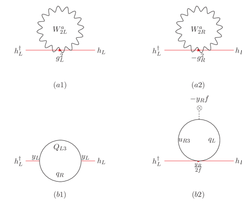
Figure 1: Diagrams responsible for the cancellation of one loop quadratically divergent contributions to the Higgs mass. Diagrams (a1) and (a2) are contributions from ${\rm SU}(2)_{L}$ and ${\rm SU}(2)_{R}$ gauge bosons respectively. Diagrams (b1) and (b2) are contributions from light top and heavy top respectively.

These cancellations can be shown explicitly at one loop by using the Lagrangian and the expressions for the nonlinear Higgs fields given in the previous sections. As we are to demonstrate the cancellation of the quadratic divergence, we can treat all particles as massless and ignore the mixing between particles. The nonlinear Higgs fields $H_{L}$ and $H_{R}$ can be expanded as

$$H_{L}=h_{L}+\cdots,\ \ \ H_{R}=\left(\begin{array}[]{c}0\\ f-\frac{h_{L}^{\dagger}h_{L}}{2f}\end{array}\right)+\cdots\ .$$ (60)

Let us first examine the contributions from the ${\rm SU}(2)_{L,R}$ gauge interactions. The result can be easily extended to the case of ${\rm U}(1)$. Actually, the ${\rm U}(1)_{B-L}$ preserves the global U(4) symmetry and should not by itself contribute to the Goldstone boson potential at all. For the gauge field loop contributions, the relevant vertices come from the gauge interactions:

$$|D_{\mu}H_{L}|^{2}+|D_{\mu}H_{R}|^{2}\rightarrow g^{2}_{2L}H_{L}^{\dagger}(W_{2L}^{\dagger}W_{2L})H_{L}+g^{2}_{2R}H_{R}^{\dagger}(W_{2R}^{\dagger}W_{2R})H_{R}$$

$$=g^{2}_{2L}h_{L}^{\dagger}(W_{2L}^{\dagger}W_{2L})h_{L}+g^{2}_{2R}(0,f-\frac{h_{L}^{\dagger}h_{L}}{2f})(W_{2R}^{\dagger}W_{2R})\left(\begin{array}[]{c}0\\ f-\frac{h_{L}^{\dagger}h_{L}}{2f}\end{array}\right)+\cdots$$ (63)

$$=g^{2}_{2L}h_{L}^{\dagger}(W_{2L}^{\dagger}W_{2L})h_{L}-g^{2}_{2R}(h_{L}^{\dagger}h_{L})(W_{2R}^{\dagger}W_{2R})_{22}+\cdots$$

$$=\frac{1}{4}g^{2}_{2L}h_{L}^{\dagger}h_{L}(W_{2L}^{a\dagger}W_{2L}^{a})-\frac{1}{4}g^{2}_{2R}(h_{L}^{\dagger}h_{L})(W_{2R}^{a\dagger}W_{2R}^{a})+\cdots$$ (64)

where the gauge fields $W_{2L,2R}=W_{2L,2R}^{a}\frac{\sigma^{a}}{2}$, and the subscript (22) denotes the (2,2) component of the $W_{2R}^{\dagger}W_{2R}$. The first term generates a diagram as shown in figure 1.(a1) and the second term generates a diagram as shown in figure 1.(a2). If $g_{2L}=g_{2R}$, the two diagrams give the same amplitude and cancel each other exactly due to the minus sign of the second term.

For the top loop contributions, the relevant vertices come from the Yukawa interactions

$$y_{L}\bar{Q}_{L3}\tau_{2}H_{L}^{*}q_{R}+y_{R}\bar{Q}_{R3}\tau_{2}H_{R}^{*}q_{L}+h.c.$$ (65)

$$\sim y_{L}\bar{Q}_{L3}\tau_{2}h_{L}^{*}q_{R}-y_{R}\bar{u}_{R3}q_{L}(f-\frac{h_{L}^{\dagger}h_{L}}{2f}+...)+h.c.+\cdots$$

$$= y_{L}\bar{Q}_{L3}\tau_{2}h_{L}^{*}q_{R}-y_{R}f\bar{u}_{R3}q_{L}+\frac{y_{R}}{2f}\bar{u}_{R3}q_{L}{h_{L}^{\dagger}h_{L}}+h.c.+\cdots\ .$$

The first term generates the usual diagram as shown in figure. 1.(b1), with a contribution proportional to $-y_{L}^{2}$. The third term generates a diagram as shown in figure. 1.(b2), with a insertion of $-y_{R}f\bar{u}_{R3}q_{L}$, which is necessary as we have no $\bar{u}_{R3}q_{L}$ propagator in the massless limit. Such diagram gives a contribution proportional to $-\frac{y_{R}}{2f}\times(-y_{R}f)\times 2$, where the factor of two takes into account the contribution from the third term and its Hermitian conjugate. The quadratic divergences in Fig. 1.(b1) and (b2) cancel each other if $y_{L}=y_{R}$.

IV Mass spectrum

The new particles in the LRTH model are: heavy gauge bosons $Z_{H}$, $W_{H}^{\pm}$, heavy top quark $T$, neutral Higgs $\phi^{0}$, a pair of charged Higgses $\phi^{\pm}$, and a ${\rm SU}(2)_{L}$ complex Higgs doublet: $\hat{h}_{1}^{\pm}$, $\hat{h}_{2}^{0}$. The model parameters are the Higgs vevs $f$, $\hat{f}$, the top quark Yukawa $y$, the cut off scale $\Lambda$, the top quark vector singlet mass mixing parameter $M$, a mass parameter $\mu_{r}$ for $\phi^{0}$, and a mass parameter $\hat{\mu}$ for $\hat{h}_{1}^{\pm}$ and $\hat{h}_{2}^{0}$. Once $f$ is fixed, the vev $\hat{f}$ can be determined by minimizing the CW potential for the SM Higgs and requiring that the SM Higgs obtains an electroweak symmetry breaking vev of 246 GeV. The top Yukawa $y$ can be fixed by the light top quark mass. The remaining free parameters are: ($f$, $\Lambda$, $M$, $\mu_{r}$ and $\hat{\mu}$).

The value of $f$ and $\hat{f}$ are bounded from below by electroweak precision measurements, which will be discussed in sec. V. It cannot be too large either since the fine tuning is more severe for larger $f$. In our analysis below, we pick $f$ to be in the range of 500 GeV $-$ 1.5 TeV. The corresponding fine tuning is in the range of 27% to 4%. The cut off scale $\Lambda$ is typically chosen to be $4\pi f$. Sometime $\Lambda=2\pi f$ is also considered. The mass mixing between the vector top single, $M$, controls the amount of ${\rm SU}(2)_{L}$ singlet $q_{L}$ in the SM-like light top $t$. It is therefore constrained by the $Z\bar{b}b$ coupling and oblique parameters. On the other hand, nothing forbids $M$ to be set to zero, which corresponds to zero mixing between the light top quark and heavy top quark. The collider phenomenology for $M=0$ or very small value of $M$ ($\lesssim$ 1 GeV) differs dramatically from larger value of $M$, which will be discussed separately in Sec. VII. The value for $\mu_{r}$ is non-zero, otherwise the neutral Higgs $\phi^{0}$ is massless. The value of $\mu_{r}$ cannot be too large either, since otherwise the fine tuning of the SM Higgs mass becomes severe. In our analysis, we pick $\mu_{r}$ to be small, as the current experimental bound on the mass of $\phi^{0}$ is fairly weak. The parameter $\hat{\mu}$ sets the masses for the Higgses $\hat{h}_{1}^{\pm}$, $\hat{h}_{2}^{0}$. Such a mass term breaks the left-right symmetry softly, and could be of the order of $f$. Although it is not particularly relevant for collider studies, it controls the mass of the dark matter candidate $\hat{h}_{2}^{0}$ and plays an important role in the dark matter relic density analysis suDM .

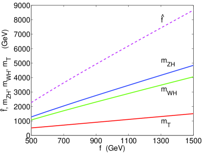
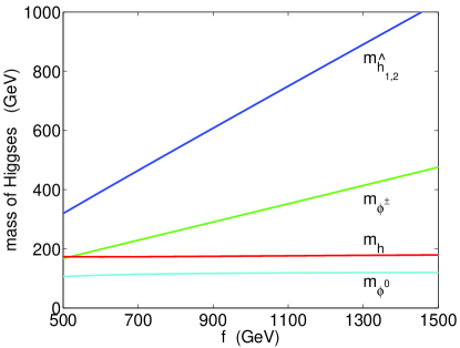
Figure 2: The left plot shows the value of $\hat{f}$ and masses of $Z_{H}$, $W_{H}$ and $T$. The right plot shows the masses of $\hat{h}_{1}^{\pm}$ ($\hat{h}_{2}^{0}$), $\phi^{\pm}$, $h$ and $\phi^{0}$. The other parameters are chosen as $\Lambda=4\pi f$, $M=150$ GeV, $\mu_{r}=50$ GeV and $\hat{\mu}=f/2$.

Fig. 2 shows the masses of the new particles as a function of $f$, for a typical set of parameter choices of $\Lambda=4\pi f$, $M=150$ GeV, $\mu_{r}=50$ GeV and $\hat{\mu}=f/2$. The top curve in the left plot of Fig. 2 shows the value of $\hat{f}$ as a function of $f$, which is determined from the minimization of the CW potential of the SM Higgs. The heavy top mass, which is determined by $f$, is between 500 GeV and 1.5 TeV. The heavy gauge boson masses are above 1 TeV, heavier than the heavy top. This is because the heavy gauge boson masses are controlled by a much larger vev $\hat{f}$. This mass hierarchy is different from the spectrum of the littlest Higgs model littest , where the heavy top is heavier than the heavy $W_{H}$ lhtao . The masses of $W_{H}$ and $Z_{H}$ in the LRTH model are related: $m_{W_{H}}=m_{Z_{H}}\sqrt{\cos 2\theta_{w}}/\cos\theta_{w}$. This mass relation is also different from the littlest Higgs model, where $m_{W_{H}}=m_{Z_{H}}$. Choosing $\Lambda=2\pi f$ instead of $4\pi f$ leads to larger values of $\hat{f}$. The masses for $W_{H}$ and $Z_{H}$ also become heavier, due to their $\hat{f}$ dependence. The mass of the heavy top remains unchanged, since it is independent of $\hat{f}$. All of those particles are within the reach of the LHC.

The right plot of Fig. 2 shows the masses for all the Higgses in the LRTH model. The mass of the Higgs $\phi^{0}$ is related to $\mu_{r}$ as $m_{\phi^{0}}=\mu_{r}\sqrt{\hat{f}/f}$. For $\mu_{r}=50$ GeV, the mass for $\phi^{0}$ is around 100 GeV. The masses of the charged Higgses $\phi^{\pm}$ obtain contributions from both the $\mu_{r}$ term, similar to the neutral Higgs $\phi^{0}$, and the CW potential, $(g^{4}/16\pi^{2})\hat{f}^{2}\ln\Lambda^{2}/(g^{2}\hat{f}^{2})$. Their masses increase with $f$, and are between 200 to 400 GeV. The SM Higgs mass is determined by the CW potential. It varies between 145 $-$ 180 GeV, depending slightly on the values of $\Lambda$ and $M$. The masses of the Higgses $\hat{h}_{1}^{\pm}$ and $\hat{h}_{2}^{0}$ are nearly degenerate, with a small splitting caused by the electromagnetic interactions. Three individual pieces contribute to its mass squared: $\hat{\mu}^{2}$, $\mu_{r}^{2}(f/\hat{f})$ and terms from the CW potential. The CW contribution is between $(200{\rm\ GeV})^{2}$ to $(700{\rm\ GeV})^{2}$ for $f$ varies between 500 GeV to 1500 GeV. For smaller values of $\Lambda$, all the Higgs masses except $\phi^{0}$ decrease. For $\phi^{0}$, the mass increases slightly, due to the larger value of $\hat{f}$. the LHC reach of these particles depends on their production processes and decay modes, which will be discussed in Sec. VI.

For smaller value of $M$, $\hat{f}$ decreases. This leads to a slightly smaller value for $m_{W_{H}}$, $m_{Z_{H}}$ and all the Higgs masses. The heavy top mass also decreases due to the smaller splitting between the light and heavy tops.

V Experimental constraints

The strongest experimental constraints on the LRTH model come from the precision measurements on the virtual effects of heavy gauge bosons, and the mass bounds from the direct searches at high energy colliders.

The constraints on the mass of the heavy $W_{H}$ depend on the masses of the right handed neutrinos. For $m_{\nu_{R}}<m_{e}$, $m_{W_{H}}$ is constrained to be larger than 4 TeV to avoid the over production of ${}^{4}{\rm He}$ nucleo . For $m_{\nu_{eR}}<m_{p}$, supernova cooling constrains $m_{W_{H}}$ to be larger than 23 TeV supernova . However, once the right handed neutrinos are heavy, all those constraints are relaxed. In the LRTH, the right handed neutrinos could obtain large Majorana masses of the order of $\hat{f}^{2}/\Lambda$, and the above mentioned constraints on $m_{W_{H}}$ are therefore absent. The strongest constraint on $m_{W_{H}}$ then comes from $K_{L}-K_{S}$ mixing. The box diagram with the exchange of one $W$ and one $W_{H}$ has an anomalous enhancement and yields the bound $m_{W_{H}}>1.6$ TeV KLKS , which translates into a lower limit on $f$ to be 670 GeV. This analysis, however, did not include higher order QCD corrections and it used vacuum insertion to obtain the matrix element. An update on the $m_{W_{H}}$ constraints from $K_{L}-K_{S}$ mixing is under current investigation KLKSupdate . The current limit also assumes that the CKM matrix for the right handed quark sector is the same as or the complex conjugate of the one for the left handed quark sector. The bound on $m_{W_{H}}$ can further be relaxed if we drop this assumption. It will lead to a breaking of left-right symmetry in the first two generations. This is safe since no large contributions to the Higgs masses appear from the first two generation quarks due to the smallness of their Yukawa couplings. The direct search limit on $m_{W_{H}}$ depends on the masses of $\nu_{R}$. If $m_{\nu_{R}}>m_{W_{H}}$, $W_{H}\rightarrow l\nu_{R}$ is forbidden. D0 excludes the mass range of 300 to 800 GeV assuming $W_{H}$ decays dominantly into two jets D0WH . The CDF excludes the mass region of 225 to 566 GeV in $t\bar{b}$ final states CDFWH . The CDF bound is weaker for the heavy $W_{H}$ in the LRTH since the decay of $W_{H}\rightarrow{t}\bar{b}$ is suppressed by the smallness of $M$. For $m_{\nu_{R}}\ll m_{W_{H}}$, CDF finds $m_{W_{H}}>786$ GeV using the $e$ and $\mu$ final states combined CDFnuR , while the D0 limit is 720 GeV D0nuR . For $m_{\nu_{R}}=m_{W_{H}}/2$, the D0 bound weakens to 650 GeV D0nuR .

Unlike the heavy charged gauge boson $W_{H}$, which does not mix with the SM $W$, the heavy $Z_{H}$ mixes with the SM $Z$ with a mixing angle of the order of $v^{2}/\hat{f}^{2}$. There are three types of indirect constraints. $Z$-pole precision measurements constrain only the $Z-Z_{H}$ mixing. The low energy neutral current processes and high energy precision measurements off the $Z$-pole are sensitive not only to $Z-Z_{H}$ mixing, but also to the direct $Z_{H}$ exchange. The limit on the $Z-Z_{H}$ mixing is typically $<$ few $\times 10^{-3}$ PDG , translating into $\hat{f}$ ($f$) to be larger than a few TeV (500$-$600 GeV). The lower bound on the heavy $Z_{H}$ mass from precision measurements is about 500$-$800 GeV PDG . $Z_{H}$ can also be directly produced at high energy colliders and decays into quarks or leptons. In the leptonic final states, the current bounds from CDF is about 630 GeV PDG .

VI Sketches for Future Collider phenomenology

In this section, we discuss the collider phenomenology of the new particles in the LRTH model. We present the production cross sections and particle decay branching ratios. All the numerical studies are done using CalcHEP calchep . Signals typically involve multijets, energetic leptons and missing energies. The SM backgrounds are in general unsuppressed, and more detailed analyses for individual processes are needed to identify the discovery potential for the LRTH model at the LHC. Such study is beyond the scope of the current paper and we leave it for future work collidersu .

Since the decays of the particles depend on the left-right mass mixing of the top singlet $M\bar{q}_{L}q_{R}$, which therefore changes the collider signals, we first discuss the general case with a small $M$, choosing $M=150$ GeV as an illustration. For very small value of $M$ ($\lesssim$ 1 GeV), in particular, for $M=0$, the decay patterns of certain particles change dramatically, which leads to completely different collider signals. We devote Sec. VII for the discussion of such case.

VI.1 Heavy top quark

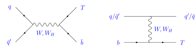
Figure 3: Feynman diagrams for single heavy top production.

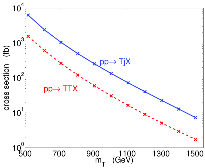
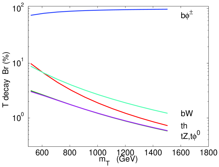
Figure 4: Left plot shows the single and pair production for heavy top quark at the LHC. The “x”’s correspond to the value of $f$ being $500,600,...,1500$ GeV. The right plot shows the branching ratios of the heavy top decay for $M=150$ GeV.

A single heavy top quark can be produced at the LHC dominantly via $s$-channel or $t$-channel $W$ or $W_{H}$ exchange, as shown in Fig. 3. The associated jet is mostly a $b$-jet in the former case, or $u/d$ jets in the latter case. Since $W_{H}$ is heavier than $T$ in the LRTH models, the $s$-channel on-shell $W_{H}$ decay dominates the single heavy top production, contributing to more than 80% of the total cross section. The contribution from $W$ boson exchange is negligible, since $W\bar{T}b$ coupling is suppressed by $(M/f)(v/f)$, which vanishes in the limit of $M=0$. This is different from the little Higgs model, where the $t$-channel $W$ exchange dominates the single heavy top production cross section.

The single heavy top quark production cross section is shown by the solid curve in the left plot of Fig. 4. For a heavy top mass of 500$-$1500 GeV, the cross section is in the range of $7\times 10^{3}$ fb $-$ 10 fb. It is comparable to the single heavy top production cross section in the littlest Higgs model lhtao , which is about 20 fb for a 1500 GeV heavy top. We also show the cross section of heavy top pair production (dashed line in the left plot of Fig. 4). The dominant contribution comes from gluon exchange: $q\bar{q},gg\rightarrow T\bar{T}$. Although the QCD coupling is larger, this channel suffers from the phase space suppression due to the large heavy top mass. The cross section is about a factor of five smaller when compared to the single heavy top production mode.

The decay branching ratios of the heavy top are shown in the right plot of Fig. 4. For $M=150$ GeV, more than 70% of heavy top decays via

$$T\rightarrow\phi^{+}+b,$$ (66)

with a partial decay width of

$$\Gamma(T\rightarrow\phi^{+}b)=\frac{1}{8\pi}\frac{p_{b}}{m_{T}}\left[{E_{b}}(|g_{L}|^{2}+|g_{R}|^{2})+{m_{b}}(g_{L}g_{R}^{*}+g_{L}^{*}g_{R})\right],$$ (67)

where $p_{b}$ and $E_{b}$ is the momentum and energy of $b$-jet in the rest frame of the heavy top and $g_{L}$ and $g_{R}$ are the left and right handed couplings of $\phi^{-}\bar{b}T$: $\phi^{-}\bar{b}(g_{L}p_{L}+g_{R}p_{R})T$, which can be read off from Table 5. In the limit of $M\ll f$, $g_{L}\sim iy$ and $g_{R}\sim im_{b}/f\sim 0$, the partial decay width simplifies to

$$\Gamma(T\rightarrow\phi^{+}b)=\frac{y^{2}}{16\pi}p_{b}\approx\frac{y^{2}}{32\pi}m_{T}.$$ (68)

In the last step, we have ignored the final state masses since they are small compared to large $m_{T}$.

Considering the subsequent decay of

$$\phi^{+}\rightarrow tb,\ \ t\rightarrow W^{+}b\rightarrow l^{+}\nu b,$$ (69)

the signal is 3 $b$-jets $+$ one charged lepton ($e$ or $\mu$) $+$ missing $E_{T}$. There is always an additional energetic jet (most likely a $b$-jet) that accompanies $T$ from single heavy top production process. Due to the large single heavy top production cross section and ${\rm Br}(W\rightarrow e\nu_{e},\mu\nu_{\mu})\sim 20\%$, more than 10,000 events can be seen with $10\ {\rm fb}^{-1}$ luminosity for a heavy top mass of around 600 GeV. The SM backgrounds come from $t\bar{t}$, $W+$4 jets and $tbj$. Preliminary study in Ref. collidersu shows that the jet associated with the single $T$ production is typically very energetic comparing to the jets from $t\bar{t}$ decays. A cut on the transverse momentum of the most energetic jet offers an effective way to suppressed the dominant $t\bar{t}$ background while retains most of the signals. In addition, the reconstruction of $W$, $t$, $\phi^{+}$ and $T$ can be used to discriminate the signal from the background. We can reconstruct the $W$ boson using the invariant mass of the lepton and neutrino . Combining the $W$ with one $b$-jet, we require the invariant mass to be around the top quark mass. Similarly, we can reconstruct $\phi^{+}$ through the combination of $tb$ and reconstruct ${T}$ using $b\phi^{+}$.

The heavy top can also decay into $ht$, $Zt$ and $Wb$. The decay branching ratios are suppressed since the relevant couplings are suppressed by at least one power of $M/f$. The $\bar{T}_{R}t_{L}h$ and $\bar{T}_{R}t_{R}Z$ couplings are proportional to the fraction of $q_{R}$ in $T_{R}$, which is about $M/f$. The $\bar{T}_{L}t_{R}h$, $\bar{T}_{L}t_{L}Z$ and $\bar{T}_{L}b_{L}W$ couplings are proportional to the fraction of $u_{L3}$ in $T_{L}$, which is about $(M/f)(v/f)$. For large $m_{T}$, the relation

$$\Gamma(T\rightarrow ht)=\Gamma(T\rightarrow Zt)=\frac{1}{2}\Gamma(T\rightarrow Wb)$$ (70)

still holds as in the littlest Higgs models lhtao , due to the Goldstone boson equivalence theorem. However, such relation is hard to test at the LHC because of the suppressed branching ratios into those channels. For $M=150$ GeV, the branching ratio for $T\rightarrow Wb$ is about 10% for $m_{T}\sim$ 500 GeV, and decreases quickly for larger $m_{T}$.

The search for $T\rightarrow Wb$ is similar to the usual single top quark searches atlasTDR ; singletop . The leptonic $W$ decay yields a nice signal of one $b$-jet $+$ one electron or muon $+$ missing $E_{T}$. For single $T$ production channel, there is usually additional energetic jet which is most likely a $b$-jet. Requiring one energetic lepton, at least two energetic jets and at least one energetic $b$-tagging jet reduces the enormous QCD multijet background atlasTDR . The remaining dominant SM backgrounds are SM single top production(via $Wt$, $W$-gluon fusion or $W^{*}$ processes), $t\bar{t}$, $Wb\bar{b}$ and $Wjj$. Studies in Ref. singletop shows that requiring no more than two jets can be used to reduce the $t\bar{t}$ and $Wt$ background, which has on average more jets than the single heavy top process. Requiring more than one $b$-tagging jet reduces the $Wjj$ and the SM $Wt$ and $W-$gluon fusion background. Since the neutrino momentum can be fully reconstructed (with a two-fold ambiguity), requiring $m_{l\nu b}$ to lie around $m_{T}$ reduces $Wjj$, $Wbb$ and single top background. Further rejection of $Wjj$ and $Wbb$ background can be achieved by impose a cut on the scalar sum of the jet $p_{T}$, which typically has a lower value. Similar analysis for $T\rightarrow Wb$ in the little Higgs models has been studied in Ref. LHCTH , and it was shown that for ${\cal L}=300\ {\rm fb}^{-1}$, 5 $\sigma$ discovery is possible for $m_{T}$ up to about 2 TeV. Note, however, that in the little Higgs model, ${\rm Br}(T\rightarrow Wb)=50$%, while in LRTH, the branching ratio is much less, depending on the values of $M$ and $f$.

At small value of $f$ around 500 GeV, the branching ratio for $T\rightarrow ht$ is about 10%. Since the mass of $h$ in the LRTH models is typically around 170 GeV, it decays dominantly into $WW^{*}$ or $ZZ^{*}$, leading to multilepton signals. The main background is top pair production, where both tops decay semileptonically and a third lepton can arise from a $b$ jet. Studies for channels with similar final states in the little Higgs models (for $V_{H}\rightarrow Vh$ with a heavy $h$) have been discussed in Ref. LHCLHVH .

The heavy top can also decay into $Zt$:

$$T\rightarrow Z+t,\ {\rm with\ }Z\rightarrow l^{+}l^{-},\ {\rm and\ }t\rightarrow W^{+}b\rightarrow l^{+}\nu b.$$ (71)

The signal is 1 $b$-jet $+$ tri-lepton $+$ missing $E_{T}$. The dominant SM background comes from $WZ$, $ZZ$ and $tbZ$. Similar studies in the framework of little Higgs models LHCTH show that requiring three isolated energetic lepton (either $e$ or $\mu$), energetic $b$-jets, missing $E_{T}$ larger than 100 GeV, and a pair of leptons with reconstructed invariant mass around $m_{Z}$ rejects most of the background. At ${\cal L}=300\ {\rm fb}^{-1}$, 5 $\sigma$ discovery at the LHC is possible for $m_{T}$ up to about 1 TeV (with ${\rm Br}(T\rightarrow Zt)=25$%). In the LRTH, however, such channel is only useful for small $f$ and not so small $M$.

The decay of

$$T\rightarrow t+\phi^{0},\ {\rm with\ }\phi^{0}\rightarrow b\bar{b},\ {\rm and\ }t\rightarrow W^{+}b\rightarrow l^{+}\nu b.$$ (72)

is also possible for small values of $f$. The signal is three $b$-jets, plus energetic lepton and missing $E_{T}$. Such process is very similar to $T\rightarrow ht$ with $h\rightarrow b\bar{b}$ in the little Higgs models LHCTH . The dominating background comes from $t\bar{t}$, which can only be distinguished by studying the kinematics. Studies LHCTH showed that the discovery in such mode is more difficult comparing to $Wb$ and $Zt$ modes that we discussed before. It can, however, be used as an confirmation if heavy top partners are discovered in other channels.

Due to the small mixing of the vector top singlet, the deviation of $Wtb$ coupling from its SM value is of the order of $(M/f)^{2}(v/f)^{2}$, which is usually less than a few percent. Such a small deviation is very hard to observe, even at a high luminosity linear collider.

VI.2 Heavy gauge bosons

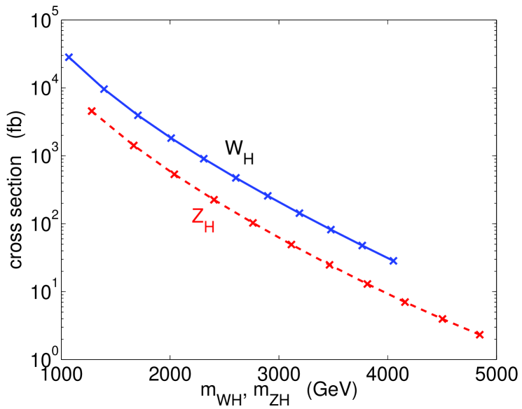
Figure 5: Cross section for heavy gauge bosons $W_{H}$ and $Z_{H}$ Drell-Yan productions at the LHC. The “x”’s correspond to the value of $f$ being $500,600,...,1500$ GeV.

The dominant production channels for heavy gauge bosons at hadron colliders are the Drell-Yan processes: $pp\rightarrow W_{H}X$ and $pp\rightarrow Z_{H}X$. The production cross sections are shown in Fig. 5. The heavy right handed $W_{H}$ boson couples to the SM light quark pairs with the SM coupling strength. The Drell-Yan cross section is large: varying from $3\times 10^{4}$ fb for $W_{H}$ mass of about 1 TeV to 30 fb for $W_{H}$ mass of about 4 TeV. For the heavy $Z_{H}$, the cross section is smaller comparing to $W_{H}$, due to the smaller $Z_{H}$ coupling to the SM fermion pairs as shown in Table 6. The cross section is still sizable: varying from $5\times 10^{3}$ fb for $Z_{H}$ mass around 1.3 TeV to 2 fb for $Z_{H}$ mass around 5 TeV.

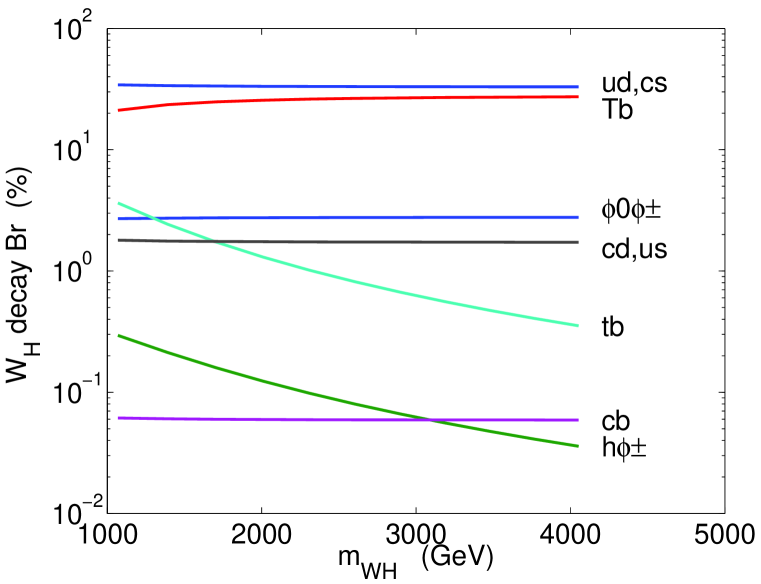
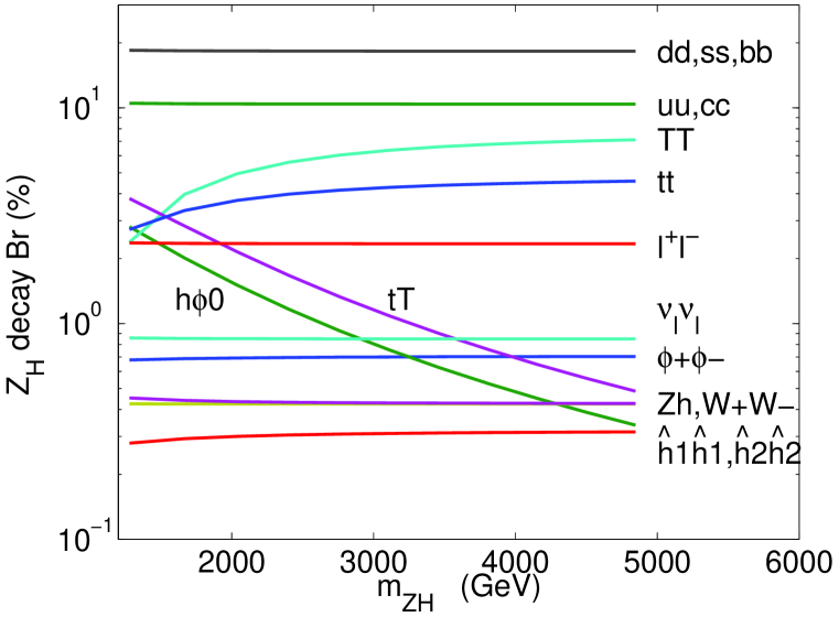
Figure 6: Decay branching ratios of the heavy gauge bosons $W_{H}$ and $Z_{H}$ for $M=150$ GeV. Here we have assumed that $m_{\nu_{R}}>m_{W_{H}}$ and the leptonic decay modes for $W_{H}$ are absent.

In Fig. 6, we show the decay branching ratios of $W_{H}$ and $Z_{H}$ as a function of the gauge boson masses. For $W_{H}$, it can not decay to the SM leptons and neutrinos since it is a purely ${\rm SU}(2)_{R}$ gauge boson. It could, however, decay into $l+\nu_{R}$ if $m_{W_{H}}>m_{\nu_{R}}$, which will be discussed later. In Fig. 6, such leptonic decay mode is absent since the right handed neutrino masses are set to be larger than $m_{W_{H}}$ in our analyses. The dominant decay mode for $W_{H}$ is into two jets, with a branching ratio of about 30%. Such mode suffers from the overwhelming QCD di-jets background for large $p_{T}$ jets dijetLHC . Current limits on dijets events from resonance decay RunIINP is relatively weak.

$W_{H}$ could also decay into a heavy top plus a $b$-jet, with a branching ratio of about 20%$-$30%. Depending on the subsequent decays of the heavy top, we expect to see signals of

• 4 $b$ + lepton ($e$ or $\mu$) + missing $E_{T}$, with a branching ratio suppression factor of ${\rm Br}(T\rightarrow\phi^{+}b)\times{\rm Br}(W\rightarrow l^{+}\nu)>14\%$. The dominant SM backgrounds are $t\bar{t}$ and $W+jjjj$.

• 2 $b$ + lepton ($e$ or $\mu$) + missing $E_{T}$, with a branching ratio suppression factor of ${\rm Br}(T\rightarrow W^{+}b)\times{\rm Br}(W\rightarrow l^{+}\nu)<2\%$. The dominant SM backgrounds are $tj$, $t\bar{t}$, $Wbb$ and $Wjj$.

• 2 $b$ + tri-lepton($e$ or $\mu$) + missing $E_{T}$, with a branching ratio suppression factor of ${\rm Br}(T\rightarrow Zt)\times{\rm Br}(W\rightarrow l^{+}\nu)\times{\rm Br}(Z\rightarrow l^{+}l^{-})<6\times 10^{-4}$. The dominant SM background is $tbZ$.

Since single $T$ production mostly comes from on-shell $W_{H}$ decay, the discussion in Sec. VI.1 for heavy top partners also applies to $W_{H}$ study here.

$W_{H}$ could also decay into $\phi^{0}\phi^{\pm}$ with a branching ratio of about 3%. This is the dominant production mode for $\phi^{0}$.

The $W_{H}\rightarrow tb$ branching ratio is of the order of 4% or less. Search of $tb$ final states from a heavy $W_{H}$ decay has been studied in Ref. sullivan . It has been shown that at the LHC, with 10$-$ 100 ${\rm fb}^{-1}$ luminosity, a reach of $m_{W_{H}}$ of $3-4$ TeV is possible at 95% C.L.

For $1\ {\rm GeV}<m_{\nu_{R}}<m_{W_{H}}$, where the lower bound is imposed to avoid the strong constraints on the $W_{H}$ mass from either supernova cooling supernova or the relic abundance of ${}^{4}{\rm He}$, $W_{H}\rightarrow l\nu_{R}$ is possible, with a branching ratio of about 9%. $\nu_{R}$ further decays into lepton plus jets. The details of the decay process are very model dependent, which will not be further discussed here.

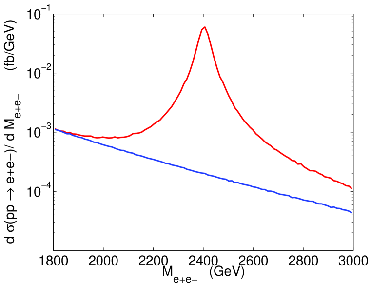
Figure 7: The invariant $e^{+}e^{-}$ mass distribution at the LHC. The blue (dark) line is for the SM background, and the red(light) line is for the LRTH model where a heavy $Z_{H}$ is produced through the Drell-Yan process. The model parameters are chosen to be $f=800$ GeV, $M=150$ GeV and $\Lambda=4\pi f$. The corresponding $Z_{H}$ mass is 2403 GeV, with a decay width of $\Gamma_{Z_{H}}=51$ GeV.

Although the dominant decay mode of $Z_{H}$ is into dijets, the discovery modes for $Z_{H}$ would be $l^{+}l^{-}$ (with a branching ratio of 2.5% for $e^{+}e^{-}$, $\mu^{+}\mu^{-}$ and $\tau^{+}\tau^{-}$ individually). The di-lepton mode $e^{+}e^{-}$ or $\mu^{+}\mu^{-}$ provides a clean signal, which can be separated from the SM background by studying the invariant dilepton mass distribution, as shown in Fig. 7. Searches for heavy neutral gauge boson in dilepton final states have been studied at both the Tevatron dileptonZH ; RunIINP ; RunIIZH and the LHC atlasTDR ; dileptonZH ; LHCZH . The current search limit from the Tevatron Run II is about 600$-$900 GeV RunIINP ; RunIIZH , while mass up to about 5 TeV could be covered at the LHC atlasTDR ; LHCZH .

The pair production of $t\bar{t}$ (with a branching ratio of 2-5%) via $Z_{H}$ decay can also be useful. Searches of $t\bar{t}$ resonance have been studied in atlasTDR ; wbwbLHC . Requiring that one $W$ decays leptonically and one $W$ decays hadronically, the signal is $l\nu bbjj$. The dominant backgrounds are $W+$jets, $Z+$jets, $t\bar{t}$ and $tbj$. Requiring large missing $E_{T}$, energetic isolated electron or muon, at least four energetic jets with at least one tagged as a $b$-jet reduces some of the backgrounds. The reconstruction of the $t\bar{t}$ resonance mass could be used to further suppress the continuum $t\bar{t}$ background. For 300 ${\rm fb}^{-1}$ integrated luminosity, $5\sigma$ discovery limit of $\sigma\times{\rm Br}$ are 835 fb, 265 fb and 50 fb for the masses of resonances being $m=$ 500 GeV, 1 TeV and 2 TeV atlasTDR . With the cross section and $t\bar{t}$ branching ratio of $Z_{H}$, the reach for $Z_{H}\rightarrow t\bar{t}$ at the LHC is only about 1 TeV, due to the small decay branching ratio into $t\bar{t}$ final states.

It is also possible to discover the heavy $Z_{H}$ gauge boson via its decaying into a pair of heavy top quarks $T\bar{T}$, with a branching ratio of 2-7%. The heavy top mostly decays into $\phi^{\pm}b$, which typically has two $W$’s and six $b$-jets in the final states. Such channel, however, also suffers from small $Z_{H}\rightarrow T\bar{T}$ branching ratio, and its LHC reach is limited.

VI.3 Higgses

VI.3.1 SM Higgs

The SM Higgs mass can be obtained via the minimization of the Higgs potential, which depends on $f(\hat{f})$, $M$ and $\Lambda$. Varying $M$ between 0 and 150 GeV, $\Lambda$ between $2\pi f$ and $4\pi f$, and $f$ between 500 GeV and 1500 GeV, the Higgs mass is found to be in the range of $145-180$ GeV. For this intermediate mass region, several channels have been studied for Higgs discovery.

The best channel for Higgs discovery at the LHC for intermediate mass region is vector boson fusion production, with $h\rightarrow WW^{*}\rightarrow l\nu l\nu$ qqH ; WBFWW . Signals for such channel are two forward tagging jets, central jet veto, energetic di-leptons and missing $E_{T}$ from neutrinos. The characteristic signatures of additional forward jets in the detector and low jet activity in the central region allow for an efficient background rejection. The remaining dominant backgrounds come from $t\bar{t}$ and QCD $\gamma^{*}/Z+$jets production with $\gamma^{*}/Z\rightarrow ll$. Requiring a tag forward jet not being tagged as $b$-jet reduces the $t\bar{t}$ background. $ee$ and $\mu\mu$ Drell-Yan backgrounds can be efficiently rejected by tightening the di-lepton mass cut and by introducing a $E_{T}^{miss}$ cut. Analyses in Ref. qqH showed that such process has a better signal-to-background ratio than $gg\rightarrow h$ with $h\rightarrow WW^{*}$ or $ZZ^{*}$ for Higgs mass between 140 GeV and 190 GeV. At ATLAS, a sensitivity of 5 $\sigma$ can be reached with an integrated luminosity of only 10 ${\rm fb}^{-1}$ in such channel.

Gluon fusion process $gg\rightarrow h$ has the largest cross section for Higgs production at the LHC. For the intermediate mass region, the so-called golden plated channel $h\rightarrow ZZ^{*}\rightarrow 4l$ made of 4$e$, 4$\mu$ and 2$e$2$\mu$ decays, provides a clean signature. The most important irreducible backgrounds are $ZZ^{*}$ and $Z\gamma^{*}$ production with decays to four leptons. The most important reducible backgrounds are $t\bar{t}$ and $Zb\bar{b}$ production. The main cuts to reduce the background are isolated leptons, a mass cut on one of the lepton pairs to be around the $Z$ mass, and a requirement for the other lepton pair to have an invariant mass above 20 GeVHZZ . It is shown that with an integrated luminosity of 30 ${\rm fb}^{-1}$, this channel may allow discovery above 5 $\sigma$ in the range of $130<m_{h}<180$ GeV atlasTDR , with an exception near 170 GeV, where this branching ratio is reduced due to the opening of $h\rightarrow WW$ decay.

In the region around 170 GeV, we can use $h\rightarrow WW^{*}\rightarrow l\nu l\nu$ channel. The irreducible backgrounds are made of $WW$ continuum, and of $WZ$ and $ZZ$. The reducible backgrounds come from $t\bar{t}$, $Wt$, $Wbb$, $b\bar{b}$ and $W+$ jet production. Requesting central jet veto, strong angular correlation between the leptons and high missing transverse mass allows us to discriminate between the signal and the background. With an integrated luminosity of 10 ${\rm fb}^{-1}$, a significance larger than 5 $\sigma$ maybe obtained in the region $150<m_{h}<190$ GeV HWW .

VI.3.2 $\phi^{0}$ and $\phi^{\pm}$

Besides the SM Higgs, there are three additional Higgses that couple to both the SM fermions and the gauge bosons: one neutral Higgs $\phi^{0}$ and a pair of charged Higgses $\phi^{\pm}$.

The light neutral Higgs boson $\phi^{0}$ is a pseudo-scalar and charged under the spontaneously broken ${\rm SU}(2)_{R}$. Its mass is a free parameter and is determined by $\mu_{r}$ that can be anything below $f$. $\phi^{0}$ can in principle be very heavy and become unobservable at the LHC. Here we consider another possibility where the mass of $\phi^{0}$ is about 100 GeV. Due to its pseudo-scalar nature, there is no $\phi^{0}W^{+}W^{-}$, $\phi^{0}ZZ$ coupling at tree level . Such couplings, similar to $\phi^{0}\gamma\gamma$ and $\phi^{0}gg$, can be generated at loop level with heavy fermions.

$\phi^{0}$ decays donimantly into $b\bar{b}$, $c\bar{c}$ or $\tau^{+}\tau^{-}$. The decay widths are proportional to the square of the corresponding Yukawa couplings, with an additional suppression factor of $v^{2}/(2f^{2})$ comparing to that of the SM Higgs. The decay branching ratio of $\phi^{0}\rightarrow b\bar{b}$, $c\bar{c}$ and $\tau^{+}\tau^{-}$, however, are close to the corresponding SM Higgs decay branching ratios, since the additional suppression factor cancels out. Given the huge QCD background in the LHC environment, the discovery of $\phi^{0}$ is difficult through those channels, unless there are other particles produced associated with $\phi^{0}$, which could provide a handle to trigger the events and to distinguish the background rainwater .

Similar to the SM Higgs, the loop generated $\phi^{0}\rightarrow\gamma\gamma$ could be useful due to the narrow $\gamma\gamma$ peak that can be reconstructed to distinguish the signal from the background. Unlike the SM Higgs, where $h\gamma\gamma$ are generated by both the top quark and $W$ loop, the one-loop SM gauge boson contribution to $\phi^{0}\gamma\gamma$ is zero because of the absence of the tree level $\phi^{0}WW$ coupling. The SM top loop contribution is also suppressed since $\phi^{0}t\bar{t}$ coupling is suppressed by small $M/f$. $\phi^{0}\gamma\gamma$ coupling, however, gets contributions from the loop with the heavy top partner $T$, with an unsuppressed $\phi^{0}T\bar{T}$ coupling. Due to the heavy top mass, heavy top quark loop contribution to $\phi^{0}\gamma\gamma$ is suppressed by a factor of $v/(\sqrt{2}f)$ comparing to the SM top contribution to $h\gamma\gamma$ for $m_{h}=m_{\phi^{0}}$. The heavy gauge boson loop contributions are absent since there is no $\phi^{0}W_{H}W_{H}$ coupling. Since the SM top loop competes with the SM $W$ loop in its contribution to $h\gamma\gamma$, the decay width of $\phi^{0}\rightarrow\gamma\gamma$ is roughly $v^{2}/(2f^{2})$ suppressed comparing to the decay width of $h\rightarrow\gamma\gamma$. Given that $\phi^{0}\rightarrow b\bar{b}$ is also suppressed by the same factor comparing to $h\rightarrow b\bar{b}$, the branching ratio of $\phi^{0}\rightarrow\gamma\gamma$ is roughly the same as ${\rm Br}(h\rightarrow\gamma\gamma$) for $m_{h}=m_{\phi^{0}}$.

The associated production of $\phi^{0}$ with $W$ or $Z$ is suppressed by a loop factor comparing to the usual Higgsstrahlung production at the LHC, due to the absence of the tree level $\phi^{0}WW$ and $\phi^{0}ZZ$ coupling. The dominant production is again the gluon fusion process $gg\rightarrow\phi^{0}$ with a heavy top loop. Similar to $\phi^{0}\gamma\gamma$ coupling that discussed above, gluon fusion production of $\phi^{0}$ is suppressed by a factor of $v^{2}/(2f^{2})$ comparing to that of the SM Higgs with the same mass. The total number of event of $gg\rightarrow\phi^{0}\rightarrow\gamma\gamma$ is then suppressed by a factor of $v^{2}/(2f^{2})$ comparing to the SM process $gg\rightarrow h\rightarrow\gamma\gamma$. Studies for the SM Higgs discovery in this channel atlasTDR ; CMSHiggs showed that a 5$\sigma$ discovery of a light (115 GeV) SM Higgs requires an integrated luminosity of about 25 ${\rm fb}^{-1}$ at the LHC. Since the significance level scales as $(\sigma\times{\rm Br})_{\rm signal}\times\sqrt{\cal L}$, a factor of 9 suppression of the $\phi^{0}$ signal cross section (for a low value of $f\sim$ 500 GeV) is very hard to compensate with an increasing luminosity.

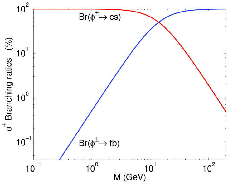
Figure 8: The decay branching ratios of $\phi^{\pm}\rightarrow tb$ and $\phi^{\pm}\rightarrow cs$, as a function of $M$. The model parameters are chosen to be $f=800$ GeV, $\mu_{r}=50$ GeV, and $\Lambda=4\pi f$.

The charged Higgses $\phi^{\pm}$ dominantly decay into $tb$ or $cs$, with the decay width of the former channel proportional to $(M/f)^{2}$, and the decay width of the latter channel proportional to the charm Yukawa coupling squared. Fig. 8 shows the branching ratios of $\phi^{\pm}\rightarrow tb$ and $\phi^{\pm}\rightarrow cs$ as a function of $M$. It is clear that for larger value of $M$, $\phi^{\pm}\rightarrow tb$ dominates. If the particles produced associated with $\phi^{\pm}$ do not involve leptons, the $W$ from top decay is required to decay leptonically, which can be used as a trigger, and also to suppress the background. For very small value of $M$ $\lesssim$ 1 GeV, ${\rm Br}(\phi^{\pm}\rightarrow tb)$ drops to less than 1% and $\phi^{\pm}\rightarrow cs$ dominates, which leads to completely different phenomenology. We defer the discussion of such case together with $M=0$ limit to Sec.VII.

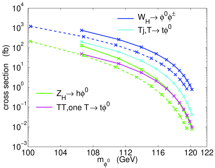
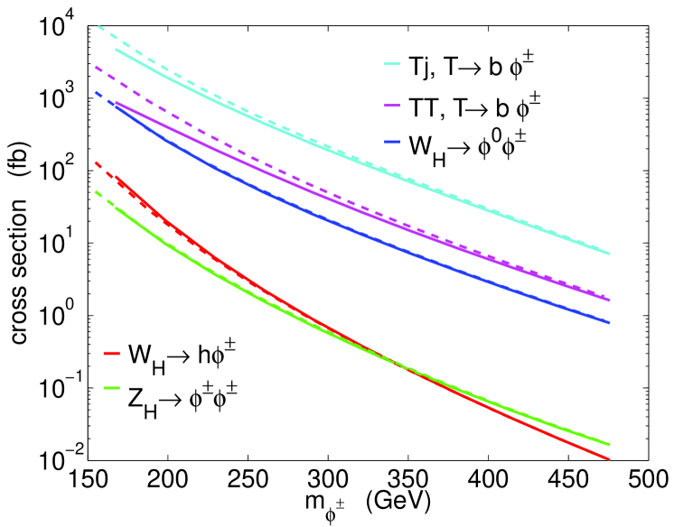
Figure 9: The production of $\phi^{0}$ (left plot) and $\phi^{\pm}$ (right plot) from the decay of heavy particles at the LHC. The solid lines are for $M=150$ GeV, while the dashed lines are for $M=0$. In the left plot, from top to bottom, the production modes are $W_{H}\rightarrow\phi^{0}\phi^{\pm}$, single $T$ production with $T\rightarrow t\phi^{0}$, $Z_{H}\rightarrow h\phi^{0}$ and $TT$ pair production with one heavy top decaying into $\phi^{0}$ while the other top decaying into anything. In the right plot, from top to bottom (for small $m_{\phi^{\pm}}$), the production modes are single $T$ production with $T\rightarrow b\phi^{\pm}$, $TT$ pair production with both heavy tops decaying into $b\phi^{\pm}$, $W_{H}\rightarrow\phi^{0}\phi^{\pm}$, $W_{H}\rightarrow h\phi^{\pm}$, and $Z_{H}\rightarrow\phi^{+}\phi^{-}$. The other parameters are chosen to be $\Lambda=4\pi f$ and $\mu_{r}=50$ GeV. The “x”’s in the left plot correspond to the value of $f$ being $500,600,...,1500$ GeV.

The heavy particles in the LRTH models, $W_{H}$, $Z_{H}$, and $T$, can decay into the light Higgses. Due to the large Drell-Yan cross sections for $W_{H}$ and $Z_{H}$, and the large single $T$ production cross section at the LHC, the production of $\phi^{0}$ and $\phi^{\pm}$ from the decay of heavy particles could be sizable, as shown in Fig. 9. Notice that the fall of the cross section for heavier Higgs mass is due to the reduction of $W_{H}$, $Z_{H}$ and $T$ production cross sections with increasing $f$.

For the neutral Higgs $\phi^{0}$, the dominant production mode is through $W_{H}\rightarrow\phi^{0}\phi^{\pm}$, with a cross section of about $10^{3}$ fb $-$ 1 fb. Combined with the decay of $\phi^{0}$ and $\phi^{\pm}$, we can look for signals of 4 $b$-jets $+$ 1 lepton ($e$ or $\mu$) $+$ missing $E_{T}$. Two $b$-jets need to be chosen to reconstruct the $\phi^{0}$ mass, while $\phi^{\pm}$ can be reconstructed as described above. $\phi^{0}$ produced from the heavy top decay: $T\rightarrow t\phi^{0}$, might also be used to identify the neutral Higgs.

For the charged Higgses $\phi^{\pm}$, the dominant production mode is through heavy top decay, since the branching ratio for $T\rightarrow\phi^{\pm}b$ is more than 70%. The cross section is in the range of $6\times 10^{3}$ fb $-$ 10 fb. Considering the single heavy top production $pp\rightarrow TjX$, with $T\rightarrow\phi^{\pm}b$, the signal is 3 $b$-jets $+$ 1 jet $+$ 1 lepton ($e$ or $\mu$) $+$ missing $E_{T}$. The top quark from $\phi^{\pm}$ decay can be reconstructed through $bW$, while $\phi^{\pm}$ can be reconstructed through $tb$. The reconstructed invariant mass for $tb$ could also tell us the mass of $\phi^{\pm}$.

$\phi^{0}$ and $\phi^{\pm}$ can also be produced in association with the third generation quarks: $b\bar{b}\phi^{0,\pm}$, $t\bar{t}\phi^{0,\pm}$, $tb\phi^{0,\pm}$. The cross sections are usually much smaller than the ones that are mentioned above, and therefore are not discussed further.

VI.3.3 $\hat{h}_{1}^{\pm}$ and $\hat{h}_{2}^{0}$

The complex charged and neutral Higgses $\hat{h}_{1}^{\pm}$ and $\hat{h}_{2}^{0}$ couple to the gauge bosons only. Their masses are very degenerate, with a small mass splitting of about 100 $-$ 700 MeV introduced by the electro-magnetic interactions. The charged Higgses $\hat{h}_{1}^{\pm}$ are slightly heavier than the neutral one, and can therefore decay into $\hat{h}_{2}^{0}$ plus soft jets or leptons. If the decay happens inside the detector, the jets and leptons are so soft that they cannot be detected at colliders. The neutral Higgs $\hat{h}_{2}^{0}$ is stable and escapes the detector, and therefore appears as a missing energy signal. It is, however, a good dark matter candidate. The study of $\hat{h}_{2}^{0}$ as a viable dark matter candidate is left to future studies suDM .

The production cross sections of $\hat{h}_{1}^{\pm}$ and $\hat{h}_{2}^{0}$ at the LHC are relatively small. They can only be pair produced via the exchange of photon, $Z$, $W$, $Z_{H}$, or Higgses. The cross sections are about 1 fb. The collider signatures depend on the lifetime of $\hat{h}_{1}^{\pm}$, which further depends on the mass splitting $\Delta{M}$ between $\hat{h}_{1}^{\pm}$ and $\hat{h}_{2}^{0}$. For small $\Delta{M}<m_{\pi}$, the decay lifetime of $\hat{h}_{1}^{\pm}$ is relatively long and the decay of $\hat{h}_{1}^{\pm}\rightarrow\hat{h}_{2}^{0}$ happens outside the detector. $\hat{h}_{1}^{\pm}$ appears as a charged track in the detector with little hadronic activities. It can be distinguished from the muon background by requiring a large ionization rate $dE/dx$ or using the time of flight information. Such signal is hard to miss since it is almost background free. For an extensive review on the collider searches of a long lived stable particle, see Ref. stable . For $\Delta{M}\sim m_{\pi}$, $\hat{h}_{1}^{\pm}$ decay inside the detector while leaving a track in the tracking chamber, such events could be identified with a disappearing track. To trigger on such events, we need to look at the associated production of $\hat{h}_{1}^{\pm}$ with a jet. For larger $\Delta{M}$, $\hat{h}_{1}^{\pm}$ decay instantly inside the detector, the soft jets and leptons escape the detection, and the missing $E_{T}$ is balanced in the pair production. Such events are very difficult to detect since there is no visible final states to be observed. Similar studies for degenerate winos in the anomaly-mediated supersymmetry breaking scenario have been done in the literature wino .

VII Collider phenomenology with $M=0$ or very small value of $M$

All the above discussions are for small but sizable value of $M$. From Eq. (45), the top quark mass eigenstates $t$ and $T$ are related to the gauge eigenstates $u_{3L},u_{3R},q_{L},q_{R}$ by the mixing angle $\alpha_{L}$ and $\alpha_{R}$. In the limit of $M=0$, $\sin\alpha_{L}=0$ and $\sin\alpha_{R}=0$. Therefore, the SM top quark is purely $(u_{3L},q_{R})$, and the heavy top is purely $(q_{L},u_{3R})$. Certain couplings vanish at this limit, as shown in Table 1. The couplings that vanish at $M=0$ are proportional to $M/f$. We will discuss below the collider phenomenology of $M=0$ case. They can also be applied to the case when $M$ deviates from zero slightly: $M\lesssim 1$ GeV.

The main phenomenological difference between the $M=0$ case and the case discussed in the previous section comes from the decay modes of $\phi^{\pm}$. Because of the absence of $\phi^{+}\bar{t}b$ coupling, $\phi^{\pm}$ can no longer decay into $tb$. $\phi^{\pm}$ cannot decay into ${T}b$ either since $m_{T}>m_{\phi^{\pm}}$. The previous subdominant channel $\phi^{\pm}\rightarrow cs$ now becomes the main decay mode, leading to all jet final states. For nonzero value of $M$, Fig. 8 shows that $\phi^{\pm}\rightarrow cs$ becomes dominant (${\rm Br}(\phi^{\pm}\rightarrow tb)<1\%$) when $M\lesssim 1$ GeV. The discovery of $\phi^{\pm}$ becomes extremely difficult at the LHC, due to the huge QCD jet background.

Due to the absence of certain couplings in the $M=0$ limit, some production processes for $\phi^{0}$ disappear. The cross sections for $\phi^{0}$ from the decay of heavy particles for $M=0$ are given in the dashed lines of the left plot of Fig. 9. No contribution from $T$ decay is present since $Tt\phi^{0}$ coupling is zero. For the same $m_{\phi^{0}}$, the cross section for $M=0$ is smaller than non-zero $M$ case. However, when we compare the cross section with the same value of $f$, the one for $M=0$ is actually larger. This is because $\hat{f}$ is smaller for $M=0$ case, which leads to a smaller mass for the heavy gauge boson $W_{H}$ and $Z_{H}$ and a larger Drell-Yan cross section. The decay of $\phi^{0}$ is still the same as before: $\phi^{0}\rightarrow b\bar{b},c\bar{c},\tau\bar{\tau}$. $\phi^{0}$ is dominantly produced associated with $\phi^{\pm}$ from $W_{H}$ decay. This channel is not so useful for $\phi^{0}$ discovery at the LHC since both $\phi^{0}$ and $\phi^{\pm}$ decay hadronically. The cross section for $\phi^{0}$ produced associated with a SM Higgs from $Z_{H}$ decay is about a factor of 10 smaller than $\phi^{0}\phi^{\pm}$ production. The leptonic final states from Higgs decay might make this channel useful for $\phi^{0}$ discovery.

The cross sections for $\phi^{\pm}$ production from heavy particle decays for $M=0$ are presented in the dashed lines in the right plot of Fig. 9. For $\phi^{\pm}$ production from heavy top decay, the cross section is larger than the non-zero $M$ case, this is mainly because the branching ratio for $T\rightarrow\phi^{+}b$ is larger, now 100%. The discovery of $\phi^{\pm}$, however, is very difficult, because $\phi^{\pm}$ dominantly decay hadronically. The suppressed $h\phi^{\pm}$ production from $W_{H}$ decay might become important for $\phi^{\pm}$ studies.

For the heavy top, both the single and pair heavy top production cross sections do not change much. However, the heavy top decay is affected. The only two body decay mode is now $T\rightarrow b\phi^{+}$, with a branching ratio of 100%. The other decay channels: $T\rightarrow bW^{+}$, $T\rightarrow tZ$, $T\rightarrow t\phi^{0}$ and $T\rightarrow th$ are forbidden since the relevant couplings are zero. Due to the dominant hadronic decay of $\phi^{\pm}$ for $M=0$, the discovery of the heavy top quark also becomes difficult at the LHC.

The situation is different for the $W_{H}$ and $Z_{H}$. The Drell-Yan cross section for $W_{H}$ and $Z_{H}$ do not change much since they only depend on the masses of the heavy gauge bosons. The decays of $W_{H}$ and $Z_{H}$ almost do not change, except that ${\rm Br}(W_{H}\rightarrow tb)={\rm Br}(Z_{H}\rightarrow Tt)=0$. These two branching ratios are small for non-zero $M$ (less than a few percent). Shutting off these two decay modes does not change the branching ratio of other decay channels that much. The dilepton signal and $t\bar{t}$ signal for $Z_{H}$ do not change. For $W_{H}$, its discovery potential depends on the masses of $\nu_{R}$. If $m_{\nu_{R}}<m_{W_{H}}$, $W_{H}$ can be studied using dilepton plus jets signal from $W_{H}\rightarrow l\nu_{R}$ process. If $m_{\nu_{R}}>m_{W_{H}}$, however, $W_{H}$ discovery also becomes challenge at the LHC. The study of its decay to $Tb$ is very hard due to the difficulty of identifying $T$, as discussed above. Signals suffer from either huge QCD background or small cross sections for processes with leptonic final states.

VIII Conclusion

The twin Higgs mechanism provides an alternative method to solve the little hierarchy problem. In this paper, we present in detail the embedding of the twin Higgs mechanism in LRTH models. There are TeV scale heavy top and heavy gauge bosons, which interact with SM quarks, leptons and gauge bosons. There are also additional Higgses in the model. The neutral Higgs $\phi^{0}$ and charged Higgses $\phi^{\pm}$ couple to the SM quarks, leptons and gauge bosons. There is an extra ${\rm SU}(2)_{L}$ Higgs doublet $(\hat{h}_{1}^{+},\hat{h}_{2}^{0})$, which couples to the gauge sector only. The lighter one $\hat{h}_{2}^{0}$ is stable, which could be a good dark matter candidate.

The collider phenomenology of the LRTH depends sensitively on the parameter $M$, which is the mass mixing between the vector heavy top singlet. The discovery potential at the LHC for $M\gtrsim 5$ GeV is very promising. For the heavy top, the dominant production channel at the LHC is single heavy top production in association with a jet. Heavy top dominantly decays to $\phi^{\pm}b$. The consequent decay of $\phi^{\pm}$ leads to signals of $l\nu bbbj$. The reconstruction of the intermediate on shell particles could distinguish the signal from the background. $W_{H}$ and $Z_{H}$ are produced via the Drell-Yan processes. If $\nu_{R}$ is too heavy for $W_{H}$ to decay into, $W_{H}$ could be discovered via $Tb$ or $tb$ channel. If $m_{\nu_{R}}<m_{W_{H}}$, $W_{H}\rightarrow l\nu_{R}$ could also be used to identify $W_{H}$. The dilepton decay mode for $Z_{H}$ provides a clean signal, although $Z_{H}$ could also be studied in $t\bar{t}$ or $T\bar{T}$ channel.

The mass of the SM Higgs is in the range of 145$-$180 GeV. Its discovery via $ZZ^{*}$ or $WW^{*}$ is promising at the LHC. The charged Higgses $\phi^{\pm}$ and the neutral Higgs $\phi^{0}$ are most likely to be discovered in the decay products of heavy particles. The charged Higgses $\phi^{\pm}$, which are largely produced in $T$ decay, decays dominantly to $tb$. The discovery for $\phi^{0}$ is much more difficult. It can be produced from $W_{H}\rightarrow\phi^{0}\phi^{\pm}$, and decays dominantly into $b\bar{b}$.

The Higgses $\hat{h}_{1}^{\pm}$ and $\hat{h}_{2}^{0}$ can only be pair produced via electroweak processes at the LHC. Their masses are very degenerate, and $\hat{h}_{1}^{\pm}$ decay to $\hat{h}_{2}^{0}$ plus soft leptons or jets. The collider signatures depend strongly on the mass splitting $\Delta{M}$ between $\hat{h}_{1}^{\pm}$ and $\hat{h}_{2}^{0}$. If $\Delta{M}\lesssim m_{\pi}$, the decay lifetime of $\hat{h}_{1}^{\pm}$ is relatively long. We will see either isolated track in the tracking chamber with little hadronic activities, or disappearing tracks. Otherwise, both the soft jets or leptons, and the missing energy from $\hat{h}_{2}^{0}$ escape the detection. It becomes difficult to identify $\hat{h}_{1}^{\pm}$ and $\hat{h}_{2}^{0}$ at the LHC. The stable $\hat{h}_{2}^{0}$ could be a good dark matter candidate. Its relic density analysis and the direct and indirect detection potential are under current investigation suDM .

If the mixing $M$ between the vector top singlet is very small $\lesssim 1$ GeV, the mixings between the two top quark gauge eigenstates are negligible. Certain couplings, for example, $\phi^{\pm}tb$, go to zero, which leads to dramatic changes in the collider phenomenology. Most of the signals discussed for sizable $M$ suffer from either huge QCD jet background, or small cross sections for signals with leptonic final states. The only exceptions are $W_{H}$ (if $m_{\nu_{R}}<m_{W_{H}}$) and $Z_{H}$, which can still be discovered via Drell-Yan production and their leptonic decays.

There are further studies can be performed in the LRTH model. In this paper, we analyze the productions of new particles and the general feature of their decay patterns. A more realistic analysis would include both the signal and the background, and the choices of appropriate cuts to either trigger the events, and/or to suppress the background. Therefore, it is worthwhile to pick typical decay processes and study in detail the LHC reach of the LRTH model. For example, for heavy top, the dominant production mode is single heavy top production $pp\rightarrow TjX$, with the subsequent decay of $T\rightarrow\phi^{+}b,\ \ \phi^{+}\rightarrow t\bar{b},\ \ t\rightarrow W^{+}b\rightarrow l^{+}\nu b.$ The collider signal is three $b$-jets $+$ one jet $+$ one lepton $+$ missing $E_{T}$. More than 10,000 events can be seen at $10\ {\rm fb}^{-1}$ luminosity for a heavy top of around 600 GeV. Detailed study need to be done to optimize the cuts and identify the signal from the background collidersu .

It is also important to identify, experimentally, the twin Higgs mechanism. In particular, the equality of the left and right Yukawa couplings. A careful examination of the cancellation between the quadratically divergent contributions from SM-like light top and heavy top quark shows that the following leading order relation needs to be satisfied:

$$y_{L}^{2}-\frac{y_{R}}{f}m_{T}=0$$ (73)

Therefore, to identify the twin Higgs mechanism, it is essential to testify this relation at colliders. The left Yukawa coupling $y_{L}$ could be obtained from the SM top quark mass $y_{L}=\sqrt{2}m_{t}/v$. The mass of the heavy top $m_{T}$ can be reconstructed from the heavy top decay chain. Knowing $m_{T}$, the right Yukawa coupling $y_{R}$ can be obtained from the heavy top decay width $\Gamma(T\rightarrow\phi^{+}b)$ using Eq. (68). The value of $f$ could be derived from $m_{T}$ and $y_{R}$ using the relation that $f=m_{T}/y_{R}$. Studies on testifying the twin Higgs mechanism along this direction are under current investigation mechanismsu .

The collider signatures of the LRTH model could mimic signals of the little Higgs models. Both classes of models have similar particle content: heavy top and heavy gauge bosons. If we see heavy top and heavy gauge bosons at collider, it is important to identify whether they are the ones from the LRTH, or the ones from the little Higgs models. There are several handles that we can use to distinguish these two models, for example, the mass relation between heavy top and heavy gauge bosons, and the decay pattern of the heavy top quark. The Higgs sector of the LRTH might also mimic that of two Higgs doublet models. Further studies are needed to distinguish those scenarios.

Appendix A Higgs fields in unitary gauge

The scalar fields of the nonlinear sigma model can be parameterized by

$$H=fe^{i\frac{\pi}{f}}\left(\begin{array}[]{c}0\\ 0\\ 0\\ 1\\ \end{array}\right),\ \ \ \ \pi=\left(\begin{array}[]{cccc}-N/2&0&0&h_{1}\\ 0&-N/2&0&h_{2}\\ 0&0&-N/2&C\\ h_{1}^{*}&h_{2}^{*}&C^{*}&3N/2\\ \end{array}\right),$$ (74)

where $\pi$ are the corresponding Goldstone fields. $N$ is a neutral real pseudoscalar, $C$ and $C^{*}$ is a pair of charged complex scalar fields, and $(h_{1},h_{2})$ is the SM ${\rm SU}(2)_{L}$ Higgs doublet. They together comprise the seven Goldstone bosons. Similar expression can be written down for Higgs field $\hat{H}$ with Goldstone fields $\hat{\pi}$.

Re-summing the exponential expansions, these Goldstone boson fields can be parameterized by

$$H=i\frac{\sin\sqrt{\chi}}{\sqrt{\chi}}e^{i\frac{N}{2f}}\left(\begin{array}[]{c}h_{1}\\ h_{2}\\ C\\ N-if\sqrt{\chi}\cot\sqrt{\chi}\\ \end{array}\right),\ \ \hat{H}=i\frac{\sin\sqrt{\hat{\chi}}}{\sqrt{\hat{\chi}}}e^{i\frac{\hat{N}}{2\hat{f}}}\left(\begin{array}[]{c}\hat{h}_{1}\\ \hat{h}_{2}\\ \hat{C}\\ \hat{N}-i\hat{f}\sqrt{\hat{\chi}}\cot\sqrt{\hat{\chi}}\\ \end{array}\right),$$ (75)

where $\chi=(h_{1}^{\dagger}h_{1}+h_{2}^{\dagger}h_{2}+C^{*}C+N^{2})/f^{2}$ and similarly for $\hat{\chi}$. It can be shown explicitly that this parametrization has a canonically normalized kinetic term for every Goldstone field except $N$, which has a kinetic term $\frac{9}{4}(\partial{N})^{2}$. The normalization can be fixed by making the change $N\rightarrow\frac{\sqrt{2}}{3}N$. We will fix the normalization later when we go to the unitary gauge and redefine the physical Higgs fields.

We have to know which combinations of these scalars are eaten by massive gauge bosons in order to go to the unitary gauge. This can be done by investigating the gauge-Higgs mixing terms arising from the covariant kinetic terms of $H$ and $\hat{H}$. We require all gauge-Higgs mixing terms vanish after the redefinition of the Higgs fields. The following re-parametrization corresponds to correct unitary gauge choice and are canonically normalized:

$$\begin{array}[]{ll}N~{}\rightarrow\frac{\sqrt{2}\hat{f}}{F(\cos x+2\frac{\sin x}{x})}\phi^{0},&~{}\hat{N}~{}\rightarrow-\frac{\sqrt{2}f\cos x}{3F}\phi^{0},\\ h_{1}\rightarrow 0,&~{}h_{2}\rightarrow\frac{v+h}{\sqrt{2}}-i\frac{x\hat{f}}{\sqrt{2}F(\cos x+2\frac{\sin x}{x})}\phi^{0},\\ C~{}\rightarrow-\frac{x\hat{f}}{F\sin x}\phi^{+},&~{}\hat{C}~{}\rightarrow\frac{{f\cos x}}{F}\phi^{+}.\\ \end{array}$$ (79)

In these expressions, we define $F=\sqrt{f^{2}\cos^{2}x+\hat{f}^{2}}$ and $x=\frac{v}{\sqrt{2}f}$.

Appendix B Mass formulas and mixing angles

For completeness, we present the exact expressions of the masses and mixing matrices for both the gauge and the top sector.

The masses for the massive gauge bosons are

$$m^{2}_{W} = \frac{1}{2}g_{2}^{2}f^{2}\sin^{2}x,$$ (80)

$$m^{2}_{W_{H}} = \frac{1}{2}g_{2}^{2}(\hat{f}^{2}+f^{2}\cos^{2}x),$$ (81)

$$m_{Z}^{2} = \frac{g_{2}^{2}+g_{Y}^{2}}{g_{2}^{2}}m_{W}^{2}\frac{2m^{2}_{W_{H}}}{m^{2}_{W_{H}}+m^{2}_{W}+\sqrt{(m^{2}_{W_{H}}-m^{2}_{W})^{2}+4\frac{g_{1}^{4}}{(g_{1}^{2}+g_{2}^{2})^{2}}m^{2}_{W_{H}}m^{2}_{W}}},$$ (82)

$$m_{Z_{H}}^{2} = \frac{g_{1}^{2}+g_{2}^{2}}{g_{2}^{2}}(m^{2}_{W_{H}}+m^{2}_{W})-m_{Z}^{2},$$ (83)

The mixing matrix $U$ between the neutral gauge bosons defined in Eq. (27) has the form

$$U = \left(\begin{array}[]{ccc}\frac{m^{2}_{W_{H}}}{\sqrt{N^{+}}(m^{2}_{Z_{H}}-m^{2}_{W_{H}})}&\frac{m^{2}_{W}}{\sqrt{N^{+}}(m^{2}_{Z_{H}}-m^{2}_{W})}&-\frac{g_{2}}{\sqrt{N^{+}}g_{1}}\\ -\frac{m^{2}_{W_{H}}}{\sqrt{N^{-}}(m^{2}_{W_{H}}-m^{2}_{Z})}&\frac{m^{2}_{W}}{\sqrt{N^{-}}(m^{2}_{Z}-m^{2}_{W})}&-\frac{g_{2}}{\sqrt{N^{-}}g_{1}}\\ \frac{g_{1}}{\sqrt{2g_{1}^{2}+g_{2}^{2}}}&\frac{g_{1}}{\sqrt{2g_{1}^{2}+g_{2}^{2}}}&\frac{g_{2}}{\sqrt{2g_{1}^{2}+g_{2}^{2}}}\\ \end{array}\right).$$ (87)

$U$ is an unitary matrix with $N^{\pm}$ being the normalization factors.

The masses for the light and heavy top quarks are

$$m_{t}^{2} = \frac{1}{2}(M^{2}+y^{2}f^{2}-N_{t}),$$ (88)

$$m_{T}^{2} = \frac{1}{2}(M^{2}+y^{2}f^{2}+N_{t}),$$ (89)

where $N_{t}=\sqrt{(y^{2}f^{2}+M^{2})^{2}-y^{4}f^{4}\sin^{2}2x}$.

The mixing angles $\alpha_{L}$ and $\alpha_{R}$ between top quarks defined in Eq. (45) are

$$\sin\alpha_{L} = \frac{1}{\sqrt{2}}\sqrt{1-(y^{2}f^{2}\cos 2x+M^{2})/N_{t}},$$ (90)

$$\sin\alpha_{R} = \frac{1}{\sqrt{2}}\sqrt{1-(y^{2}f^{2}\cos 2x-M^{2})/N_{t}}.$$ (91)

The field dependent squared masses of the gauge bosons and top quarks are needed for the calculation of the CW potential. The masses for the charged gauge bosons and top quarks are:

$$m^{2}_{W} = \frac{1}{2}g_{2}^{2}(H_{L}^{\dagger}H_{L}+\hat{H}_{L}^{\dagger}\hat{H}_{L}),$$ (92)

$$m^{2}_{W_{H}} = \frac{1}{2}g_{2}^{2}(H_{R}^{\dagger}H_{R}+\hat{H}_{R}^{\dagger}\hat{H}_{R}),$$ (93)

$$m_{t}^{2} = \frac{1}{2}(M^{2}+f^{2}y^{2}-\sqrt{(M^{2}+f^{2}y^{2})^{2}-4y^{4}|H_{L}|^{2}(f^{2}-|H_{L}|^{2})},$$ (94)

$$m_{T}^{2} = \frac{1}{2}(M^{2}+f^{2}y^{2}+\sqrt{(M^{2}+f^{2}y^{2})^{2}-4y^{4}|H_{L}|^{2}(f^{2}-|H_{L}|^{2})},$$ (95)

where $H_{L(R)}$ is the upper (lower) two components of the Higgs $H$ in Eq. (75), and similarly for $\hat{H}_{L(R)}$.

For the squared masses of the neutral gauge bosons $Z$, $Z_{H}$ and $\gamma$, we have to solve the following equation

$$\lambda^{3}+a\lambda^{2}+b\lambda+c=0$$ (96)

where

$$a = -\frac{g_{1}^{2}+g_{2}^{2}}{2}(f^{2}+\hat{f}^{2}),$$ (97)

$$b = \frac{2g_{1}^{2}+g_{2}^{2}}{g_{2}^{2}}m_{W}^{2}m_{W_{H}}^{2}-{\cal P}_{L}-{\cal P}_{R},$$ (98)

$$c = P_{R}m_{W}^{2}+P_{L}m_{W_{H}}^{2},$$ (99)

$${\cal P}_{L} = (g_{1}g_{2})^{2}\left[|H_{L}^{\dagger}\hat{H}_{L}|^{2}-(H_{L}^{\dagger}H_{L})(\hat{H}_{L}^{\dagger}\hat{H}_{L})\right],$$ (100)

$${\cal P}_{R} = (g_{1}g_{2})^{2}\left[|H_{R}^{\dagger}\hat{H}_{R}|^{2}-(H_{R}^{\dagger}H_{R})(\hat{H}_{R}^{\dagger}\hat{H}_{R})\right].$$ (101)

Note that $m_{W}^{2}$ and $m_{W_{H}}^{2}$ appear in the equations above are both field dependent.

All the physical Higgses get masses from both the soft left-right symmetry breaking $\mu$-terms, and the one-loop radiative corrections. Here we list the masses for various Higgses:

$$m_{\phi^{0}}^{2} = \frac{\mu_{r}^{2}}{F^{2}}f\hat{f}\left[\frac{\hat{f}^{2}(\cos x+\frac{\sin x}{x}(3+x^{2}))}{f^{2}(\cos x+\frac{\sin x}{x})^{2}}+2\cos x+\frac{f^{2}\cos^{2}x(1+\cos x)}{2\hat{f}^{2}}\right],$$ (102)

$$m_{\phi^{\pm}}^{2} = \frac{3}{16\pi^{2}}\frac{g_{1}^{2}m_{W_{H}}^{2}}{m_{Z_{H}}^{2}-m_{Z}^{2}}\left[(\frac{m_{W}^{2}}{m_{Z_{H}}^{2}}-1){\cal Z}(m_{Z_{H}})-(\frac{m_{W}^{2}}{m_{Z}^{2}}-1){\cal Z}(m_{Z})\right]$$ (103)

$$+\frac{\mu_{r}^{2}}{F^{2}}f\hat{f}\left[\frac{\hat{f}^{2}x}{f^{2}\sin x}+2\cos x+\frac{f^{2}\cos^{3}x}{\hat{f}^{2}}\right],$$

$$m_{\hat{h}_{2}}^{2} = \frac{3}{16\pi^{2}}\left[\frac{m_{W}^{2}}{x^{2}f^{2}}({\cal Z}(m_{W})-{\cal Z}(m_{W_{H}}))+\frac{2g_{1}^{2}+g_{2}^{2}}{4}\frac{m_{W_{H}}^{2}-m_{W}^{2}}{m_{Z_{H}}^{2}-m_{Z}^{2}}({\cal Z}(m_{Z})-{\cal Z}(m_{Z_{H}}))\right]$$ (104)

$$+\mu_{r}^{2}\frac{f}{\hat{f}}\cos x+\hat{\mu}^{2},$$

$$m_{\hat{h}_{1}}^{2} = {m}^{2}_{\hat{h}_{2}}+\frac{3}{16\pi^{2}}\frac{g_{1}^{2}m_{W}^{2}}{m_{Z_{H}}^{2}-m_{Z}^{2}}\left[(\frac{m_{W_{H}}^{2}}{m_{Z_{H}}^{2}}-1){\cal Z}(m_{Z_{H}})-(\frac{m_{W_{H}}^{2}}{m_{Z}^{2}}-1){\cal Z}(m_{Z})\right].$$ (105)

where

$${\cal Z}(x) = -x^{2}(\ln\frac{\Lambda^{2}}{x^{2}}+1).$$ (106)

We omit the exact mass formula for the SM Higgs since we obtain it from the numerical calculation when minimizing the CW potential.

Appendix C Feynman rules for interactions

In this section, we listed the new vertices which are relevant to collider physics at the LHC but are not present in the SM. The interactions are obtained via expanding the non-linear Higgs fields in Eq. (75) up to the fifth order and keeping the leading order terms in interactions.

In Table 2, we listed the interactions from covariant Higgs kinetic term ${\cal L}_{H}$. Those include (i) gauge boson-scalar-scalar interactions, (ii) gauge boson-gauge boson-scalar interactions (iii) tri-scalar interactions. For gauge boson-scalar-scalar interactions that are not Hermitian, the complex conjugate terms can be obtained by flipping the sign of the real part of the coefficients, while keep the imaginary part unchanged. In Table 3, we listed gauge boson-gauge boson-scalar-scalar interactions. For terms that are not Hermitian, the complex conjugate terms can be obtained by taking the complex conjugation of the coefficients.

There are nonrenormalizable vertices which are not listed here but are included in the numerical calculations, for example, (i) gauge boson-scalar-scalar-scalar interactions, and (ii) scalar four point interactions. These vertices are of the order of $p/f$ and $(p/f)^{2}$, for $p$ being the momentum of particles.

There are also vertices from the one-loop CW potential. These vertices contain three- and four- point scalar self-interactions. These vertices are important compared to the similar interactions from the kinetic term only at low energy since they are suppressed by loop factor $\frac{1}{16\pi^{2}}$ while the latter is proportional to the particle momentum. In our numerical calculations, the Higgs self-interactions from CW potentials are also included. The contribution from those interactions are usually small.

$\hat{h}_{1}^{\dagger}~{}\hat{h}_{2}~{}W^{+}_{\mu}$	$-e(p1-p2)_{\mu}/(\sqrt{2}s_{w})$
$\hat{h}_{1}^{\dagger}~{}\hat{h}_{1}~{}Z_{\mu}$	$-e(c_{w}^{2}-s_{w}^{2})(p1-p2)_{\mu}/(2c_{w}s_{w})$
$\hat{h}_{2}^{\dagger}~{}\hat{h}_{2}~{}Z_{\mu}$	$~{}~{}e(p1-p2)_{\mu}/(2c_{w}s_{w})$
$\phi^{-}~{}\phi^{+}~{}A_{\mu}$	$-e(p1-p2)_{\mu}$
$\phi^{-}~{}\phi^{+}~{}Z_{\mu}$	$~{}~{}e(p1-p2)_{\mu}s_{w}/c_{w}$
$h~{}\phi^{0}~{}Z_{\mu}$	$i~{}e~{}x~{}p3_{\mu}/(6c_{w}s_{w})$
$h~{}\phi^{0}~{}Z_{H\mu}$	$i~{}e~{}x((14-17s_{w}^{2})p2_{\mu}-(4-s_{w}^{2})p1_{\mu})/(18s_{w}c_{w}c2_{w})$
$\phi^{-}~{}\phi^{+}~{}Z_{H\mu}$	$-e(1-3s_{w}^{2})(p1-p2)_{\mu}/(2s_{w}c_{w}c2_{w})$
$\hat{h}_{1}^{\dagger}~{}\hat{h}_{1}~{}Z_{H\mu}$	$~{}~{}e(p1-p2)_{\mu}s_{w}/(2c_{w}c2_{w})$
$\hat{h}_{2}^{\dagger}~{}\hat{h}_{2}~{}Z_{H\mu}$	$~{}~{}e(p1-p2)_{\mu}s_{w}/(2c_{w}c2_{w})$
$\phi^{-}~{}\phi^{0}~{}W_{H\mu}^{+}$	$-e(2p2-p1)_{\mu}/(3s_{w})$
$h~{}\phi^{-}~{}W_{H\mu}^{+}$	$i~{}e~{}x(2p2-p1)_{\mu}/(3s_{w})$
$\hat{h}_{1}^{\dagger}~{}\hat{h}_{1}~{}A_{\mu}$	$-e(p1-p2)_{\mu}$
$h~{}Z_{\mu}~{}Z_{\nu}$	$~{}~{}em_{W}g_{\mu\nu}/(c_{w}^{2}s_{w})$
$h~{}Z_{\mu}~{}Z_{H\nu}$	$e^{2}f~{}x~{}g_{\mu\nu}/(\sqrt{2}c_{w}^{2}c2_{w})$
$h~{}Z_{H\mu}~{}Z_{H\nu}$	$-e^{2}f~{}x~{}g_{\mu\nu}/(\sqrt{2}c_{w}^{2}s_{w}^{2})$
$h~{}W^{+}_{\mu}~{}W^{-}_{\nu}$	$~{}~{}em_{W}g_{\mu\nu}/s_{w}$
$h~{}W_{H\mu}^{+}~{}W_{H\nu}^{-}$	$-e^{2}f~{}x~{}g_{\mu\nu}/(\sqrt{2}s_{w}^{2})$
$\phi^{-}~{}\phi^{+}~{}h$	$~{}~{}x(p3\cdot p3+2p1\cdot p2)/(3\sqrt{2}f)$
$\phi^{-}~{}\phi^{+}~{}\phi^{0}$	$i~{}p3\cdot(p2-p1)/(3\sqrt{2}f)$
$h~{}\phi^{0}~{}\phi^{0}$	$~{}~{}x(30p2\cdot p3+11p1\cdot p1)/(27\sqrt{2}f)$
$\hat{h}_{1}^{\dagger}~{}\hat{h}_{1}~{}\phi^{0}$	$i~{}f~{}p3\cdot(p1-p2)/(3\sqrt{2}\hat{f}^{2})$
$\hat{h}_{2}^{\dagger}~{}\hat{h}_{2}~{}\phi^{0}$	$i~{}f~{}p3\cdot(p1-p2)/(3\sqrt{2}\hat{f}^{2})$

Table 2: New scalar self interactions and scalar-gauge boson interactions from the covariant kinetic terms of the Higgses. $p1$, $p2$ and $p3$ refer to the incoming momentum of the first, second and third particle, respectively.

$h~{}h~{}W^{+}_{\mu}~{}W^{-}_{\nu}$	$~{}~{}e^{2}g_{\mu\nu}/(2s_{w}^{2})$	$h~{}h~{}W^{+}_{H\mu}~{}W^{-}_{H\nu}$	$-e^{2}g_{\mu\nu}/(2s_{w}^{2})$
$h~{}h~{}Z_{\mu}~{}Z_{\nu}$	$~{}~{}e^{2}g_{\mu\nu}/(2c_{w}^{2}s_{w}^{2})$	$h~{}h~{}Z_{H\mu}~{}Z_{H\nu}$	$-e^{2}g_{\mu\nu}/(2c_{w}^{2}s_{w}^{2})$
$h~{}h~{}Z_{\mu}~{}Z_{H\nu}$	$~{}~{}e^{2}g_{\mu\nu}/(2c_{w}^{2}c2_{w})$
$\phi^{0}~{}\phi^{0}~{}W^{+}_{\mu}~{}W^{-}_{\nu}$	$-e^{2}x^{2}g_{\mu\nu}/(54s_{w}^{2})$	$\phi^{0}~{}\phi^{0}~{}W^{+}_{H\mu}~{}W^{-}_{H\nu}$	$~{}~{}e^{2}x^{2}g_{\mu\nu}/(54s_{w}^{2})$
$\phi^{0}~{}\phi^{0}~{}Z_{\mu}~{}Z_{\nu}$	$-e^{2}x^{2}g_{\mu\nu}/(54s_{w}^{2}c_{w}^{2})$	$\phi^{0}~{}\phi^{0}~{}Z_{H\mu}~{}Z_{H\nu}$	$~{}~{}e^{2}x^{2}g_{\mu\nu}/(54s_{w}^{2}c_{w}^{2})$
$\phi^{0}~{}\phi^{0}~{}Z_{\mu}~{}Z_{H\nu}$	$-e^{2}x^{2}g_{\mu\nu}/(54c_{w}^{2}c2_{w})$
$\phi^{-}~{}\phi^{0}~{}W^{+}_{H\mu}~{}A_{\nu}$	$-e^{2}g_{\mu\nu}/(3s_{w})$	$\phi^{-}~{}h~{}W^{+}_{H\mu}~{}A_{\nu}$	$-2ie^{2}xg_{\mu\nu}/(3s_{w})$
$\phi^{-}~{}\phi^{0}W^{+}_{H\mu}~{}Z_{\nu}$	$~{}~{}e^{2}g_{\mu\nu}/(3c_{w})$	$\phi^{-}~{}h~{}W^{+}_{H\mu}~{}Z_{\nu}$	$~{}~{}2ie^{2}xg_{\mu\nu}/(3c_{w})$
$\phi^{-}~{}\phi^{0}W^{+}_{H\mu}~{}Z_{H\nu}$	$~{}~{}e^{2}g_{\mu\nu}/(3c_{w}c2_{w})$	$\phi^{-}~{}h~{}W^{+}_{H\mu}~{}Z_{H\nu}$	$~{}~{}2ie^{2}xg_{\mu\nu}/(3c_{w}c2_{w})$
$\phi^{-}~{}\phi^{+}~{}Z_{\mu}~{}Z_{\nu}$	$~{}~{}2e^{2}s_{w}^{2}g_{\mu\nu}/c_{w}^{2}$	$\phi^{-}~{}\phi^{+}~{}A_{\mu}~{}A_{\nu}$	$~{}~{}2e^{2}g_{\mu\nu}$
$\phi^{-}~{}\phi^{+}~{}Z_{\mu}~{}Z_{H\nu}$	$-e^{2}(3c_{w}^{2}-2)g_{\mu\nu}/(c2_{w}c_{w}^{2})$	$\phi^{-}~{}\phi^{+}~{}Z_{\mu}~{}A_{\nu}$	$-2e^{2}s_{w}g_{\mu\nu}/c_{w}$
$\phi^{-}~{}\phi^{+}~{}Z_{H\mu}~{}Z_{H\nu}$	$-2e^{2}g_{\mu\nu}/c_{w}^{2}$	$\phi^{-}~{}\phi^{+}~{}Z_{H\mu}~{}A_{\nu}$	$~{}~{}e^{2}(3c_{w}^{2}-2)g_{\mu\nu}/(c2_{w}c_{w}s_{w})$
$\phi^{-}~{}\phi^{+}~{}W^{+}_{\mu}~{}W^{-}_{\nu}$	$-e^{2}x^{2}g_{\mu\nu}/(6s_{w}^{2})$	$\phi^{-}~{}\phi^{+}~{}W^{+}_{H\mu}~{}W^{-}_{H\nu}$	$~{}~{}e^{2}x^{2}g_{\mu\nu}/(6s_{w}^{2})$
$\hat{h}_{1}^{\dagger}~{}\hat{h}_{1}~{}W^{+}_{\mu}~{}W^{-}_{\nu}$	$~{}~{}e^{2}g_{\mu\nu}/(2s_{w}^{2})$	$\hat{h}_{2}^{\dagger}~{}\hat{h}_{2}~{}W^{+}_{\mu}~{}W^{-}_{\nu}$	$~{}~{}e^{2}g_{\mu\nu}/(2s_{w}^{2})$
$\hat{h}_{1}^{\dagger}~{}\hat{h}_{1}~{}W^{+}_{H\mu}~{}W^{-}_{H\nu}$	$-e^{2}g_{\mu\nu}/(2s_{w}^{2})$	$\hat{h}_{2}^{\dagger}~{}\hat{h}_{2}~{}W^{+}_{H\mu}~{}W^{-}_{H\nu}$	$-e^{2}g_{\mu\nu}/(2s_{w}^{2})$
$\hat{h}_{1}^{\dagger}~{}\hat{h}_{1}~{}Z_{\mu}~{}Z_{\nu}$	$~{}~{}e^{2}c2_{w}^{4}g_{\mu\nu}/(2c_{w}^{2}s_{w}^{2})$	$\hat{h}_{2}^{\dagger}~{}\hat{h}_{2}~{}Z_{\mu}~{}Z_{\nu}$	$~{}~{}e^{2}g_{\mu\nu}/(2s_{w}^{2}c_{w}^{2})$
$\hat{h}_{1}^{\dagger}~{}\hat{h}_{1}~{}Z_{\mu}~{}Z_{H\nu}$	$-e^{2}c2_{w}g_{\mu\nu}/(2c_{w}^{2})$	$\hat{h}_{2}^{\dagger}~{}\hat{h}_{2}~{}Z_{\mu}~{}Z_{H\nu}$	$e^{2}g_{\mu\nu}/(2c_{w}^{2}c2_{w})$
$\hat{h}_{1}^{\dagger}~{}\hat{h}_{1}~{}Z_{H\mu}~{}Z_{H\nu}$	$-e^{2}g_{\mu\nu}/(2s_{w}^{2}c_{w}^{2})$	$\hat{h}_{2}^{\dagger}~{}\hat{h}_{2}~{}Z_{H\mu}~{}Z_{H\nu}$	$-e^{2}g_{\mu\nu}/(2s_{w}^{2}c_{w}^{2})$
$\hat{h}_{1}^{\dagger}~{}\hat{h}_{1}~{}Z_{\mu}~{}A_{\nu}$	$~{}~{}e^{2}c2_{w}^{2}g_{\mu\nu}/(c_{w}s_{w})$	$\hat{h}_{1}^{\dagger}~{}\hat{h}_{1}~{}Z_{H\mu}~{}A_{\nu}$	$-e^{2}s_{w}g_{\mu\nu}/(c_{w}c2_{w})$
$\hat{h}_{1}^{\dagger}~{}\hat{h}_{1}~{}A_{\mu}~{}A_{\nu}$	$~{}~{}2e^{2}g_{\mu\nu}$
$\hat{h}_{1}^{\dagger}~{}\hat{h}_{2}W^{+}_{\mu}~{}Z_{\mu}$	$-e^{2}g_{\mu\nu}/(\sqrt{2}c_{w})$	$\hat{h}_{1}^{\dagger}~{}\hat{h}_{2}W^{+}_{\mu}~{}Z_{H\nu}$	$-e^{2}g_{\mu\nu}/(\sqrt{2}c_{w}c2_{w})$
$\hat{h}_{1}^{\dagger}~{}\hat{h}_{2}W^{+}_{\mu}~{}A_{\nu}$	$~{}~{}e^{2}g_{\mu\nu}/(\sqrt{2}s_{w})$

Table 3: Four point gauge boson-gauge boson-scalar-scalar interactions from the covariant kinetic terms of the scalar.

$A_{\mu}~{}W^{+}_{\nu}~{}W^{-}_{\eta}$	$~{}~{}e~{}F_{\mu\nu\eta}$
$Z_{\mu}~{}W^{+}_{\nu}~{}W^{-}_{\eta}$	$~{}~{}e~{}F_{\mu\nu\eta}~{}c_{w}/s_{w}$
$Z_{H\mu}~{}W^{+}_{\nu}~{}W^{-}_{\eta}$	$~{}~{}e~{}F_{\mu\nu\eta}~{}(c2_{w}s_{w}/c_{w}^{3})(m_{W}^{2}/m_{W_{H}}^{2})$
$A_{\mu}~{}W_{H\nu}^{+}~{}W_{H\eta}^{-}$	$~{}~{}e~{}F_{\mu\nu\eta}$
$Z_{\mu}~{}W_{H\nu}^{+}~{}W_{H\eta}^{-}$	$-e~{}F_{\mu\nu\eta}~{}s_{w}/c_{w}$
$Z_{H\mu}~{}W_{H\nu}^{+}~{}W_{H\eta}^{-}$	$~{}~{}e~{}F_{\mu\nu\eta}~{}c2_{w}/(s_{w}c_{w})$
$W^{+}_{\mu}~{}W^{+}_{\nu}~{}W^{-}_{\eta}~{}W^{-}_{\rho}$	$~{}~{}e^{2}~{}G_{\mu\nu\eta\rho}/s_{w}^{2}$
$W_{H\mu}^{+}~{}W_{H\nu}^{+}~{}W_{H\eta}^{-}~{}W_{H\rho}^{-}$	$~{}~{}e^{2}~{}G_{\mu\nu\eta\rho}/s_{w}^{2}$
$A_{\mu}~{}A_{\nu}~{}W^{+}_{\eta}~{}W^{-}_{\rho}$	$-e^{2}~{}G_{\mu\nu\eta\rho}$
$Z_{\mu}~{}Z_{\nu}~{}W^{+}_{\eta}~{}W^{-}_{\rho}$	$-e^{2}~{}G_{\mu\nu\eta\rho}~{}c_{w}^{2}/s_{w}^{2}$
$A_{\mu}~{}Z_{\nu}~{}W^{+}_{\eta}~{}W^{-}_{\rho}$	$-e^{2}~{}G_{\mu\nu\eta\rho}~{}c_{w}/s_{w}$
$A_{\mu}~{}Z_{H\nu}~{}W_{\eta}^{+}~{}W_{\rho}^{-}$	$-e^{2}~{}G_{\mu\nu\eta\rho}~{}(s_{w}c2_{w}/c_{w}^{3})(m_{W}^{2}/m_{W_{H}}^{2})$
$Z_{\mu}~{}Z_{H\nu}~{}W_{\eta}^{+}~{}W_{\rho}^{-}$	$-e^{2}~{}G_{\mu\nu\eta\rho}~{}(c2_{w}/c_{w}^{2})(m_{W}^{2}/m_{W_{H}}^{2})$
$Z_{H\mu}~{}Z_{H\nu}~{}W_{\eta}^{+}~{}W_{\rho}^{-}$	$-e^{2}~{}G_{\mu\nu\eta\rho}~{}(s_{w}^{2}c2_{w}^{2}/c_{w}^{6})(m_{W}^{4}/m_{W_{H}}^{4})$
$A_{\mu}~{}A_{\nu}~{}W_{H\eta}^{+}~{}W_{H\rho}^{-}$	$-e^{2}~{}G_{\mu\nu\eta\rho}$
$Z_{\mu}~{}Z_{\nu}~{}W_{H\eta}^{+}~{}W_{H\rho}^{-}$	$-e^{2}~{}G_{\mu\nu\eta\rho}~{}s_{w}^{2}/c_{w}^{2}$
$A_{\mu}~{}Z_{\nu}~{}W_{H\eta}^{+}~{}W_{H\rho}^{-}$	$~{}~{}e^{2}~{}G_{\mu\nu\eta\rho}~{}s_{w}/c_{w}$
$A_{\mu}~{}Z_{H\nu}~{}W_{H\eta}^{+}~{}W_{H\rho}^{-}$	$-e^{2}~{}G_{\mu\nu\eta\rho}~{}c2_{w}/(c_{w}s_{w})$
$Z_{\mu}~{}Z_{H\nu}~{}W_{H\eta}^{+}~{}W_{H\rho}^{-}$	$~{}~{}e^{2}~{}G_{\mu\nu\eta\rho}~{}c2_{w}/c_{w}^{2}$
$Z_{H\mu}~{}Z_{H\nu}~{}W_{H\eta}^{+}~{}W_{H\rho}^{-}$	$-e^{2}~{}G_{\mu\nu\eta\rho}~{}c2_{w}^{2}/(s_{w}^{2}c_{w}^{2})$

Table 4: Gauge self couplings with the spin structure $F_{\mu\nu\eta}=(p3-p2)_{\mu}g_{\nu\eta}+(p1-p3)_{\nu}g_{\mu\eta}+(p2-p1)_{\eta}g_{\mu\nu}$ and $G_{\mu\nu\eta\rho}=2g_{\mu\nu}g_{\eta\rho}-g_{\mu\eta}g_{\nu\rho}-g_{\mu\rho}g_{\nu\eta}$. We also use the notations $s_{w}=\sin\theta_{w}$, $c_{w}=\cos\theta_{w}$ and $c2_{w}=\sqrt{\cos 2\theta_{w}}$ of the Weinberg angle $\theta_{w}$.

The gauge self-couplings between the gauge boson mass eigenstates can be obtained from the kinetic terms for the ${\rm SU}(2)_{L}$ and ${\rm SU}(2)_{R}$ gauge bosons, using the mixing matrix $U$ for the neutral gauge bosons given in Eq. (27). In Table 4, we listed all the gauge self-interactions.

In Table 5 we listed the Higgs-fermion-fermion interactions. In Table 6, we listed the gauge-fermion-fermion interactions, where we have ignored the flavor mixing for the charge current. Note that for term which is not Hermitian, the Hermitian conjugate term must also be added. This can be done by taking the complex conjugate of the coefficient and, for the Higgs-fermion-fermion interactions, exchanging $P_{L}\leftrightarrow P_{R}$.

$h~{}\bar{t}~{}t$	$-em_{t}C_{L}C_{R}/(2m_{W}s_{w})$
$h~{}\bar{T}~{}t$	$-y((C_{L}S_{R}+S_{L}C_{R}x)P_{L}+(C_{L}S_{R}x+S_{L}C_{R})P_{R})/\sqrt{2}$
$h~{}\bar{T}~{}T$	$-y(S_{R}S_{L}-C_{L}C_{R}x)/\sqrt{2}$
$\phi^{0}~{}\bar{T}~{}t$	$-iy(S_{L}C_{R}P_{L}-C_{L}S_{R}P_{R})/\sqrt{2}$
$\phi^{0}~{}\bar{T}~{}T$	$-iyC_{L}C_{R}\gamma_{5}/\sqrt{2}$
$\phi^{0}~{}\bar{t}~{}t$	$-iyS_{R}S_{L}\gamma_{5}/\sqrt{2}$
$\phi^{0}~{}\bar{b}~{}b$	$~{}~{}im_{b}\gamma_{5}/(\sqrt{2}f)$
$\phi^{0}~{}\bar{u}_{1,2}~{}u_{1,2}$	$-im_{u_{i}}\gamma_{5}/(\sqrt{2}f)$
$\phi^{0}~{}\bar{d}_{1,2}~{}d_{1,2}$	$~{}~{}im_{d_{i}}\gamma_{5}/(\sqrt{2}f)$
$\phi^{0}~{}\bar{l}~{}l$	$~{}~{}im_{l}\gamma_{5}/(\sqrt{2}f)$
$\phi^{+}~{}\bar{t}~{}b$	$-i(S_{R}m_{b}P_{L}-yS_{L}fP_{R})/f$
$\phi^{+}~{}\bar{T}~{}b$	$~{}~{}i(C_{R}m_{b}P_{L}-yC_{L}fP_{R})/f$
$\phi^{+}~{}\bar{u}_{1,2}~{}d_{1,2}$	$~{}~{}i(m_{d_{i}}P_{L}-m_{u_{i}}P_{R})/f$
$\phi^{+}~{}\bar{\nu}_{l}~{}l$	$~{}~{}im_{l}P_{L}/f$

Table 5: A summary of the new Higgs-fermion-fermion interactions. $P_{R,L}=\frac{1}{2}(1\pm\gamma_{5})$ are the chirality projection operators.

$A_{\mu}~{}\bar{T}~{}T$	$~{}~{}2e\gamma_{\mu}/3$
$Z_{\mu}~{}\bar{t}~{}t$	$~{}~{}e\gamma_{\mu}((3C_{L}^{2}-4s_{w}^{2})P_{L}-4s_{w}^{2}P_{R})/(6c_{w}s_{w})$
$Z_{\mu}~{}\bar{T}~{}T$	$-e\gamma_{\mu}(4s_{w}^{2}-3S_{L}^{2}P_{L})/(6c_{w}s_{w})$
$Z_{\mu}~{}\bar{T}~{}t$	$~{}~{}e\gamma_{\mu}(C_{L}S_{L}\hat{f}^{2}c_{w}^{2}P_{L}+f^{2}x^{2}s_{w}^{2}C_{R}S_{R}P_{R})/(2\hat{f}^{2}c_{w}^{3}s_{w})$
$W^{+}_{\mu}~{}\bar{t}~{}b$	$~{}~{}e\gamma_{\mu}C_{L}P_{L}/(\sqrt{2}s_{w})$
$W^{+}_{\mu}~{}\bar{T}~{}b$	$~{}~{}e\gamma_{\mu}S_{L}P_{L}/(\sqrt{2}s_{w})$
$W_{H\mu}^{+}~{}\bar{T}~{}b$	$~{}~{}e\gamma_{\mu}C_{R}P_{R}/(\sqrt{2}s_{w})$
$W_{H\mu}^{+}~{}\bar{t}~{}b$	$-e\gamma_{\mu}S_{R}P_{R}/(\sqrt{2}s_{w})$
$W_{H\mu}^{+}~{}\bar{u}_{1,2}~{}d_{1,2}$	$~{}~{}e\gamma_{\mu}P_{R}/(\sqrt{2}s_{w})$
$W_{H\mu}^{+}~{}\bar{\nu}_{l}~{}l$	$~{}~{}e\gamma_{\mu}P_{R}/(\sqrt{2}s_{w})$
$Z_{H\mu}~{}\bar{t}~{}t$	$-e\gamma_{\mu}((1+3S_{L}^{2})s_{w}^{2}P_{L}-(3c_{w}^{2}S_{R}^{2}-4s_{w}^{2})P_{R})/(6c_{w}c2_{w}s_{w})$
$Z_{H\mu}~{}\bar{T}~{}t$	$~{}~{}e\gamma_{\mu}(C_{L}S_{L}s_{w}^{2}P_{L}-C_{R}S_{R}c_{w}^{2}P_{R})/(2s_{w}c_{w}c2_{w})$
$Z_{H\mu}~{}\bar{T}~{}T$	$-e\gamma_{\mu}((3C_{L}^{2}+1)s_{w}^{2}P_{L}-(3c_{w}^{2}C_{R}^{2}-4s_{w}^{2})P_{R})/(6c_{w}c2_{w}s_{w})$
$Z_{H\mu}~{}\bar{b}~{}b$	$-e\gamma_{\mu}(s_{w}^{2}P_{L}+(3-5s_{w}^{2})P_{R})/(6s_{w}c_{w}c2_{w})$
$Z_{H\mu}~{}\bar{u}_{1,2}~{}u_{1,2}$	$-e\gamma_{\mu}(2s_{w}^{2}P_{L}+(1-7c2_{w}^{2})P_{R})/(12c_{w}s_{w}c2_{w})$
$Z_{H\mu}~{}\bar{d}_{1,2}~{}d_{1,2}$	$-e\gamma_{\mu}(s_{w}^{2}+(3-5s_{w}^{2})P_{R})/(6s_{w}c_{w}c2_{w})$
$Z_{H\mu}~{}\bar{l}~{}l$	$~{}~{}e\gamma_{\mu}(2s_{w}^{2}P_{L}+(1-3c2_{w}^{2})P_{R})/(4c_{w}s_{w}c2_{w})$
$Z_{H\mu}~{}\bar{\nu}_{L}~{}\nu_{L}$	$~{}~{}e\gamma_{\mu}s_{w}/(2c_{w}c2_{w})P_{L}$
$Z_{H\mu}~{}\bar{\nu}_{R}~{}\nu_{R}$	$~{}~{}e\gamma_{\mu}c_{w}/(2s_{w}c2_{w})P_{R}$
$Z_{\mu}~{}\bar{\nu}_{R}~{}\nu_{R}$	$-e\gamma_{\mu}m_{Z}^{2}s_{w}/(2c_{w}m_{W_{H}}^{2})P_{R}$

Table 6: A summary of new gauge-fermion-fermion interactions. $P_{R,L}=\frac{1}{2}(1\pm\gamma_{5})$ are the chirality projection operators. The mixing angles $C_{L}=\cos\alpha_{L}$, $C_{R}=\cos\alpha_{R}$ etc. are given in Eq. (48).

References

- (1) C. H. Llewellyn Smith, Phys. Lett. B 46, 233 (1973); D. A. Dicus and V. S. Mathur, Phys. Rev. D 7, 3111 (1973); J. M. Cornwall, D. N. Levin and G. Tiktopoulos, Phys. Rev. Lett. 30, 1268 (1973) [Erratum-ibid. 31, 572 (1973)]; Phys. Rev. D 10, 1145 (1974) [Erratum-ibid. D 11, 972 (1975)]; B. W. Lee, C. Quigg and H. B. Thacker, Phys. Rev. Lett. 38, 883 (1977); Phys. Rev. D 16, 1519 (1977); M. S. Chanowitz and M. K. Gaillard, Nucl. Phys. B 261, 379 (1985).
- (2) OPAL Collab. G. Abbiendi et. al., Eur. Phys. J. C 37 49 (2004); ALEPH Collab., A. Heister et. al., Phys. Lett. B 526 191 (2002); DELPHI Collab., J. Abdallah et. al., Eur. Phys. J C 32 145 (2004); DELPHI 2005-020-CONF-740; L3 Collab., P. Achard et. al., Phys. Lett. B 545 30 (2002).
- (3) ALEPH Collaboration, arXiv:hep-ex/0511027.
- (4) N. D. Christensen and R. Shrock, Phys. Lett. B 632, 92 (2006); T. Appelquist, N. D. Christensen, M. Piai and R. Shrock, Phys. Rev. D 70, 093010 (2004); D. D. Dietrich, F. Sannino and K. Tuominen, Phys. Rev. D 72, 055001 (2005); Phys. Rev. D 73, 037701 (2006).
- (5) R. Barbieri and A. Strumia, arXiv:hep-ph/0007265.
- (6) Z. Chacko, H. S. Goh and R. Harnik, Phys. Rev. Lett. 96, 231802 (2006); R. Barbieri, T. Gregoire and L. J. Hall, arXiv:hep-ph/0509242; Z. Chacko, Y. Nomura, M. Papucci and G. Perez, JHEP 0601, 126 (2006); R. Foot and R. R. Volkas, arXiv:hep-ph/0610013.
- (7) Z. Chacko, H. S. Goh and R. Harnik, JHEP 0601, 108 (2006); H. S. Goh and C. Krenke, in preparation.
- (8) A. Falkowski, S. Pokorski and M. Schmaltz, Phys. Rev. D 74, 035003 (2006); S. Chang, L. J. Hall and N. Weiner, arXiv:hep-ph/0604076.
- (9) D. Choudhury and D. P. Roy, Phys. Lett. B 322, 368 (1994); J. F. Gunion, Phys. Rev. Lett. 72, 199 (1994); R. M. Godbole, M. Guchait, K. Mazumdar, S. Moretti and D. P. Roy, Phys. Lett. B 571, 184 (2003); H. Davoudiasl, T. Han and H. E. Logan, Phys. Rev. D 71, 115007 (2005).
- (10) O. J. P. Eboli and D. Zeppenfeld, Phys. Lett. B 495, 147 (2000).
- (11) L. Neukermans and B. D. Girolamo, ATLAS-PHYS-2003-006.
- (12) K. Mazumdar, A. Nikitenko, CMS IN-2004/028.
- (13) P. Gagnon, ATL-PHYS-PUB-2005-011; F. Meisel, M. Duhrssen, M. Heldmann and K. Jakobs, ATL-PHYS-PUB-2006-009.
- (14) B. P. Kersevan, M. Malawski and E. Richter-Was, Eur. Phys. J. C 29, 541 (2003).
- (15) J. C. Pati and A. Salam, Phys. Rev. D 10, 275 (1974); R. N. Mohapatra and J. C. Pati, Phys. Rev. D 11, 566 (1975); R. N. Mohapatra and J. C. Pati, Phys. Rev. D 11, 2558 (1975).
- (16) Sidney R. Coleman and E. Weinberg Phys. Rev. D 7, 1888 (1973).
- (17) N. Arkani-Hamed, A. G. Cohen, E. Katz and A. E. Nelson, JHEP 0207, 034 (2002).
- (18) T. Han, H. E. Logan, B. McElrath and L. T. Wang, Phys. Rev. D 67, 095004 (2003); T. Han, H. E. Logan and L. T. Wang, JHEP 0601, 099 (2006); M. Perelstein, arXiv:hep-ph/0512128.
- (19) E. Dolle, J. Goodman and S. Su, in preparation.
- (20) G. Steigman, K. A. Olive and D. N. Schramm, Phys. Rev. Lett. 43, 239 (1979).
- (21) R. Barbieri and R. N. Mohapatra, Phys. Rev. D 39, 1229 (1989); G. Raffelt and D. Seckel, Phys. Rev. Lett. 60, 1793 (1988).
- (22) G. Beall, M. Bander and A. Soni, Phys. Rev. Lett. 48, 848 (1982).
- (23) S. Su, in preparation.
- (24) V. M. Abazov et al. [D0 Collaboration], Phys. Rev. D 69, 111101 (2004).
- (25) D. Acosta et. al. (CDF Collaboration), Phys. Rev. Lett. 90 081802 (2003).
- (26) T. Affolder et. al. (D0 Collaboration), Phys. Rev. Lett. 87 231803 (2001).
- (27) S. Abachi et. al. (D0 Collaboration), Phys. Rev. Lett. 76 3271 (1996).
- (28) W. M. Yao et al., J. Physics G 33. 1 (2006); WWW page URL: http://pdg.lbl.gov/.
-
(29)
A.Pukhov et al, Preprint INP MSU 98-41/542,arXiv:hep-ph/9908288;
A.Pukhov e-Print arXiv: hep-ph/0412191; CalcHEP code can be downloaded
at
http://www-zeuthen.desy.de/ pukhov/calchep.html. - (30) X. Miao and S. Su, in preparation.
- (31) ATLAS collaboration, ATLAS detector and physics performance, Technical design report. Vol. 2, CERN-LHCC-99-15.
- (32) D. O’Neil, B. Gonzalez-Pineiro and M. Lefebvre, ATLAS Internal Note ATL-COM-PHYS-99-011 (1999).
- (33) G. Azuelos et al., Eur. Phys. J. C 39S2, 13 (2005); J. E. Garcia [ATLAS Collaboration], arXiv:hep-ph/0405156.
- (34) F. Ledroit, arXiv:hep-ex/0610005.
- (35) A. Henriques and L. Poggioli, ATLAS Internal Note PHYS-92-010 (1992).
- (36) S. Tsuno [CDF - Run II Collaboration], arXiv:hep-ex/0502016; M. P. Giordani [CDF Collaboration], AIP Conf. Proc. 794, 115 (2005); M. P. Giordani [CDF and D0 Collaborations], Eur. Phys. J. C 33, S785 (2004); R. V. Cortabitarte [CDF Collaboration], arXiv:hep-ex/0406080.
- (37) Z. Sullivan, Phys. Rev. D 66, 075011 (2002); arXiv:hep-ph/0306266.
- (38) A. Abulencia et al. [CDF Collaboration], Phys. Rev. Lett. 95, 252001 (2005); Phys. Rev. Lett. 96, 211801 (2006).
- (39) M. Cvetic and S. Godfrey, arXiv:hep-ph/9504216. T. G. Rizzo, In the Proceedings of 1996 DPF / DPB Summer Study on New Directions for High-Energy Physics (Snowmass 96), Snowmass, Colorado, 25 Jun - 12 Jul 1996, pp NEW136.
- (40) Proc. of the ECFA Large Hadron Collider Workshop, Aachen (Germany) 1990, reports CERN 90-10 and ECFA 90-133; CMS Collaboration, G.L. Bayatian et. al., Technical Proposal, CERN/LHCC 94-38, LHCC/P1, 15 Dec., 1994; M. Dittmar, A. S. Nicollerat and A. Djouadi, Phys. Lett. B 583, 111 (2004).
- (41) J. A. Aguilar-Saavedra, Phys. Lett. B 625, 234 (2005); [Erratum-ibid. B 633, 792 (2006)].
- (42) S. Asai et al., Eur. Phys. J. C 32S2, 19 (2004).
- (43) D. L. Rainwater and D. Zeppenfeld, Phys. Rev. D 60, 113004 (1999) [Erratum-ibid. D 61, 099901 (2000)] [arXiv:hep-ph/9906218].
- (44) M. Sani, Czech. J. Phys. 55, B101 (2005).
- (45) S. Abdullin et. al., CMS-Note-2003/033.
- (46) W. Kilian, D. Rainwater and J. Reuter, arXiv:hep-ph/0609119.
- (47) CMS Collaboration, CMS Technical proposal, CERN/LHCC 94-38, CERN (1994).
- (48) M. Fairbairn, A. C. Kraan, D. A. Milstead, T. Sjostrand, P. Skands and T. Sloan, Phys. Rept. 438, 1 (2007) [arXiv:hep-ph/0611040].
- (49) J. L. Feng, T. Moroi, L. Randall, M. Strassler and S. Su, Phys. Rev. Lett. 83, 1731 (1999); M. Ibe, T. Moroi and T. T. Yanagida, arXiv:hep-ph/0610277.
- (50) S. Su, in preparation.