The Quark–Antiquark Contribution to the Fully Exclusive BFKL Evolution at NLL Accuracy

Abstract:

We calculate the quark–anti-quark contribution to the next-to-leading logarithmic corrections to the BFKL kernel, retaining the dependence on the momenta of the produced particles. This allows us to study the details of the NLL corrections. We demonstrate that the standard calculation of the NLL corrections to the scattering of two off-shell gluons includes contributions from energies far above that which is probed at LL. This explicitly violates energy and momentum conservation in the evolution and could be a source of the reported large NLL corrections. The presented calculation is a step towards combining energy and momentum conservation with full NLL accuracy in the evolution.

1 Introduction

The BFKL formalism is currently used both in the description of the small-$x$ evolution of the pdfs, and to obtain the leading logarithmic approximation (LLA) to the scattering matrix element for e.g. pure multi-jet and forward $W$+multi-jet production at hadron colliders. Even though the transverse scales involved in the two problems are very different, both applications rely on the same BFKL equation in the description of the evolution of an off-shell $t$–channel gluon by the emission of several gluons, and quark–anti-quark pairs at next-to-leading logarithmic accuracy (NLLA). Since the gluons emitted from the BFKL evolution are relatively hard when the formalism is applied to the approximation of the hard matrix element, it proves absolutely crucial to supplement the solution of the BFKL equation with energy and momentum conservation. While this is possible using the LL BFKL kernel, the derivation of the NLL BFKL kernel already contains phase space integrals over the invariant mass of two emitted gluons and a quark–anti-quark pair. In the standard analysis[1, 2], the NLL corrections are found to be size-able, and it therefore seems imperative to include them in the calculation of any quantity which is to be confronted with reality.

In this paper we will recalculate the quark-contribution to the NLL BFKL kernel in a form that will allow us to combine the evolution to full NLL accuracy with energy and momentum conservation[3]. We will use the obtained result to study the make-up of the NLL corrections. Specifically, we will show that in the standard analysis, due to the lack of energy and momentum conservation, the NLL corrections to a Reggeon-Reggeon scattering at a given energy receives contributions from significantly larger energies. This could be a significant and unintended source of the observed large NLL corrections.

In the interest of clarity and conciseness in our argumentation, we have chosen to include all intermediate results in the derivation of the NLL BFKL kernel.

2 Exclusive States to Next-to-Leading Logarithmic Accuracy

We will begin this section by recalling the results of the calculation of the NLL corrections to the BFKL kernel. In the following sections we will recalculate the quark–anti-quark contribution using a phase space slicing method, which allows us to study directly the energy dependence of the corrections to the Reggeon-Reggeon collision.

The BFKL equation governing the evolution in rapidity $y$ of an off-shell gluon exchanged in the $t$-channel can be written as

$$\frac{\partial}{\partial y}\ f(\mathbf{q}_{a},\mathbf{q}_{b},y)=\int\!\mathrm{d}^{D-2}\mathbf{q}\ K(\mathbf{q}_{a},\mathbf{q})\ f(\mathbf{q},\mathbf{q}_{b},y),$$ (1)

where $f(\mathbf{q}_{a},\mathbf{q}_{b},y)$ is the gluon Green’s function, and we have used boldface to denote transverse vectors. The BFKL kernel $K(\mathbf{q}_{1},\mathbf{q}_{2})$ is split into contributions from virtual and real corrections, embedded in the trajectory $\omega(\mathbf{q}_{1}^{2})$ and real emission kernel $K_{r}(\mathbf{q}_{1},\mathbf{q}_{2})$, respectively

$$K(\mathbf{q}_{1},\mathbf{q}_{2})=2\ \omega(\mathbf{q}_{1}^{2})\ \delta^{D-2}(\mathbf{q}_{1}-\mathbf{q}_{2})+K_{r}(\mathbf{q}_{1},\mathbf{q}_{2}).$$ (2)

The first two terms in the perturbative expansion of each of these terms are known

$$\omega(\mathbf{q}^{2})=\omega^{(1)}(\mathbf{q}^{2})+\omega^{(2)}(\mathbf{q}^{2})+\cdots,\quad K_{r}(\mathbf{q}_{1},\mathbf{q}_{2})=K_{r}^{(1)}(\mathbf{q}_{1},\mathbf{q}_{2})+K_{r}^{(2)}(\mathbf{q}_{1},\mathbf{q}_{2})+\cdots.$$ (3)

The leading contributions are given by

$$\omega^{(1)}(\mathbf{q}^{2})=-\bar{g}_{\mu}^{2}\left(\frac{2}{\varepsilon}+2\ln\frac{\mathbf{q}^{2}}{\mu^{2}}\right),\quad K_{r}^{(1)}(\mathbf{q}_{1},\mathbf{q}_{2})=\frac{4\ \bar{g}_{\mu}^{2}\ \mu^{-2\varepsilon}}{\pi^{1+\varepsilon}\ \Gamma(1-\varepsilon)}\frac{1}{(\mathbf{q}_{1}-\mathbf{q}_{2})^{2}}$$ (4)

with

$$\bar{g}_{\mu}^{2}=\frac{g_{\mu}^{2}\ N_{c}\ \Gamma(1-\varepsilon)}{(4\pi)^{2+\varepsilon}}$$ (5)

The next-to-leading logarithmic correction to the trajectory is[1]

$$\begin{split}\omega^{(2)}(\mathbf{q}^{2})=-\bar{g}_{\mu}^{4}\bigg{[}\frac{\beta_{0}}{N_{c}}\left(\frac{1}{\varepsilon^{2}}-\ln^{2}\left(\frac{\mathbf{q}^{2}}{\mu^{2}}\right)\right)+\left(\frac{67}{9}-\frac{\pi^{2}}{3}-\frac{10}{9}\frac{n_{f}}{N_{c}}\right)\left(\frac{1}{\varepsilon}+2\ln\left(\frac{\mathbf{q}^{2}}{\mu^{2}}\right)\right)\\ -\frac{404}{27}+2\zeta(3)+\frac{56}{27}\frac{n_{f}}{N_{c}}\bigg{]}\end{split}$$ (6)

and to the real emission kernel[1]

$$\begin{split}K_{r}^{(2)}(\mathbf{q}_{1},\mathbf{q}_{2})=\frac{4\ \bar{g}_{\mu}^{4}\ \mu^{-2\varepsilon}}{\pi^{1+\varepsilon}\ \Gamma(1-\varepsilon)}\Bigg{\{}\frac{1}{(\mathbf{q}_{1}-\mathbf{q}_{2})^{2}}\bigg{[}\frac{\beta_{0}}{N_{c}}\frac{1}{\varepsilon}\left(1-\left(\frac{(\mathbf{q}_{1}-\mathbf{q}_{2})^{2}}{\mu^{2}}\right)^{\varepsilon}(1-\varepsilon^{2}\frac{\pi^{2}}{6}\right)\\ +\left(\frac{(\mathbf{q}_{1}-\mathbf{q}_{2})^{2}}{\mu^{2}}\right)^{\varepsilon}\left(\frac{67}{9}-\frac{\pi^{2}}{3}-\frac{10}{9}\frac{n_{f}}{N_{c}}+\varepsilon\left(-\frac{404}{27}+14\zeta(3)+\frac{56}{27}\frac{n_{f}}{N_{c}}\right)\right)\bigg{]}\\ -\left(1+\frac{n_{f}}{N_{c}^{3}}\right)\frac{2\mathbf{q}_{1}^{2}\mathbf{q}_{2}^{2}-3(\mathbf{q}_{1}.\mathbf{q}_{2})^{2}}{16\mathbf{q}_{1}^{2}\mathbf{q}_{2}^{2}}\left(\frac{2}{\mathbf{q}_{2}^{2}}+\frac{2}{\mathbf{q}_{1}^{2}}+\left(\frac{1}{\mathbf{q}_{2}^{2}}-\frac{1}{\mathbf{q}_{1}^{2}}\right)\ln\frac{\mathbf{q}_{1}^{2}}{\mathbf{q}_{2}^{2}}\right)-\frac{1}{(\mathbf{q}_{1}-\mathbf{q}_{2})^{2}}\left(\ln\frac{\mathbf{q}_{1}^{2}}{\mathbf{q}_{2}^{2}}\right)^{2}\\ +\frac{2(\mathbf{q}_{1}^{2}-\mathbf{q}_{2}^{2})}{(\mathbf{q}_{1}-\mathbf{q}_{2})^{2}(\mathbf{q}_{1}+\mathbf{q}_{2})^{2}}\left(\frac{1}{2}\ln\left(\frac{\mathbf{q}_{1}^{2}}{\mathbf{q}_{2}^{2}}\right)\ln\left(\frac{\mathbf{q}_{1}^{2}\mathbf{q}_{2}^{2}(\mathbf{q}_{1}-\mathbf{q}_{2})^{4}}{(\mathbf{q}_{1}^{2}+\mathbf{q}_{2}^{2})^{4}}\right)+L\!\left(-\frac{\mathbf{q}_{1}^{2}}{\mathbf{q}_{2}^{2}}\right)-L\!\left(-\frac{\mathbf{q}_{2}^{2}}{\mathbf{q}_{1}^{2}}\right)\right)\\ -\left(3+\left(1+\frac{n_{f}}{N_{c}^{3}}\right)\left(1-\frac{(\mathbf{q}_{1}^{2}+\mathbf{q}_{2}^{2})^{2}}{8\mathbf{q}_{1}^{2}\mathbf{q}_{2}^{2}}-\frac{2\mathbf{q}_{1}^{2}\mathbf{q}_{2}^{2}-3\mathbf{q}_{1}^{4}-3\mathbf{q}_{2}^{4}}{16\mathbf{q}_{1}^{4}\mathbf{q}_{2}^{4}}(\mathbf{q}_{1}.\mathbf{q}_{2})^{2}\right)\right)\int_{0}^{\infty}\!\!\!\mathrm{d}x\ \frac{\ln\left|\frac{1+x}{1-x}\right|}{\mathbf{q}_{1}^{2}+x^{2}\mathbf{q}_{2}^{2}}\\ -\left(1-\frac{(\mathbf{q}_{1}^{2}-\mathbf{q}_{2}^{2})^{2}}{(\mathbf{q}_{1}-\mathbf{q}_{2})^{2}(\mathbf{q}_{1}+\mathbf{q}_{2})^{2}}\right)\left(\int_{0}^{1}\mathrm{d}z\ -\int_{1}^{\infty}\mathrm{d}z\ \right)\frac{\ln\frac{(z\mathbf{q}_{1})^{2}}{\mathbf{q}_{2}^{2}}}{(\mathbf{q}_{2}-z\mathbf{q}_{1})^{2}}\Bigg{\}},\end{split}$$ (7)

where

$$L(z)=\int_{0}^{z}\frac{\mathrm{d}t\ }{t}\ln(1-t),\quad\zeta(n)=\sum_{k=1}^{\infty}k^{-n},\quad\beta_{0}=\left(\frac{11}{3}N_{c}-\frac{2}{3}n_{f}\right).$$ (8)

The contribution to the real emission kernel at NLL accuracy has three sources: 1) the one-loop corrections to one gluon emission in multi Regge kinematics, 2) two-gluon emission in quasi multi Regge kinematics, and 3) quark–anti-quark production in quasi multi Regge kinematics:

$$K_{r}^{(2)}(\mathbf{q}_{1},\mathbf{q}_{2})=K_{r}^{(2),g}(\mathbf{q}_{1},\mathbf{q}_{2})+K_{r}^{(2),gg}(\mathbf{q}_{1},\mathbf{q}_{2})+K_{r}^{(2),q\bar{q}}(\mathbf{q}_{1},\mathbf{q}_{2})$$ (9)

It is the purpose of this paper to calculate the contribution $K_{r}^{(2),q\bar{q}}(\mathbf{q}_{1},\mathbf{q}_{2})$ in a form that retains not only the dependence on the sum of the transverse momenta of the emitted quark pair $(\mathbf{q}_{1}-\mathbf{q}_{2})$, but the dependence on the full momenta of both emitted particles.

The divergences of $K_{r}^{(2),q\bar{q}}(\mathbf{q}_{1},\mathbf{q}_{2})$ will fall into two categories; one at ${\boldmath\Delta}^{2}=(\mathbf{q}_{1}-\mathbf{q}_{2})^{2}\to 0$ regularised by the quark contribution to the trajectory at NLL, and an explicit pole for $\epsilon\to 0$, regularised by the quark contribution to $K_{r}^{(2),g}(\mathbf{q}_{1},\mathbf{q}_{2})$. The one-gluon production vertex for the collision of two Reggeised gluons at NLL accuracy can be calculated from a tree approximation for the quasi-multi-Regge kinematics combined with $t$–channel unitarity relations[4, 5, 6], or extracted directly from the one loop 5 gluon amplitude in the helicity basis[7]. Expanded in $D=4+2\varepsilon$ it is given by[8]:

$$\begin{split}&K_{r}^{(2),g}(\mathbf{q}_{1},\mathbf{q}_{2})=\frac{\bar{g}_{\mu}^{2}\mu^{-2\varepsilon}}{\pi^{1+\varepsilon}\Gamma(1-\varepsilon)}\frac{4}{\mathbf{k}_{1}^{2}}\Bigg{(}1+\bar{g}_{\mu}^{2}\Bigg{[}-2\left(\frac{\mathbf{k}_{1}^{2}}{\mu^{2}}\right)^{\varepsilon}\left(\frac{1}{\varepsilon^{2}}-\frac{\pi^{2}}{2}+2\varepsilon\zeta(3)\right)+\frac{\beta_{0}}{N_{c}}\frac{1}{\varepsilon}\\ &+\frac{3\mathbf{k}_{1}^{2}}{\mathbf{q}_{1}^{2}-\mathbf{q}_{2}^{2}}\ln\left(\frac{\mathbf{q}_{1}^{2}}{\mathbf{q}_{2}^{2}}\right)-\ln^{2}\left(\frac{\mathbf{q}_{1}^{2}}{\mathbf{q}_{2}^{2}}\right)+\left(1-\frac{n_{f}}{N_{c}}\right)\left(\frac{\mathbf{k}_{1}^{2}}{\mathbf{q}_{1}^{2}-\mathbf{q}_{2}^{2}}\left(1-\frac{\mathbf{k}_{1}^{2}(\mathbf{q}_{1}^{2}+\mathbf{q}_{2}^{2}+4\mathbf{q}_{1}.\mathbf{q}_{2})}{3(\mathbf{q}_{1}^{2}-\mathbf{q}_{2}^{2})^{2}}\right)\ln\left(\frac{\mathbf{q}_{1}^{2}}{\mathbf{q}_{2}^{2}}\right)\right)\\ &-\frac{\mathbf{k}_{1}^{2}}{6\mathbf{q}_{1}^{2}\mathbf{q}_{2}^{2}}(\mathbf{q}_{1}^{2}+\mathbf{q}_{2}^{2}+2\mathbf{q}_{1}.\mathbf{q}_{2})+\frac{(\mathbf{k}_{1}^{2})^{2}(\mathbf{q}_{1}^{2}+\mathbf{q}_{2}^{2})}{6\mathbf{q}_{1}^{2}\mathbf{q}_{2}^{2}(\mathbf{q}_{1}^{2}-\mathbf{q}_{2}^{2})^{2}}(\mathbf{q}_{1}^{2}+\mathbf{q}_{2}^{2}+4\mathbf{q}_{1}.\mathbf{q}_{2})\Bigg{]}\Bigg{)}\end{split}$$ (10)

The divergent piece from the quark contribution is simply

$$\frac{\bar{g}_{\mu}^{4}\mu^{-2\varepsilon}}{\pi^{1+\varepsilon}\Gamma(1-\varepsilon)}\frac{4}{\mathbf{\Delta}^{2}}\frac{-2}{3}\frac{n_{f}}{N_{c}}\frac{1}{\varepsilon}.$$ (11)

2.1 The Quark-antiquark Contribution to the NLL Corrections

The Reggeon-Reggeon-$q\bar{q}$-vertex can be calculated using the Feynman rules of the effective action in the high-energy limit in Ref.[9]. The contributing diagrams are shown in Fig. 2.1. The benefit of this framework of obtaining the scattering amplitudes is that it gives an immediate picture of the contributing sub-processes. However, the RR$q\bar{q}$ (or $g^{*}g^{*}q\bar{q}$) vertex can also be extracted directly from the full tree-level $gg\to ggq\bar{q}$ scattering amplitude in the helicity basis[10].

$$\parbox{56.9055pt}{\fmffile{NLLquarkantiquark2} \fmfgraph*(50,50) \fmfset{arrow_len}{3mm} \fmfset{arrow_ang}{15} \fmfpen{1pt} \fmfstraight\fmfleft{i0} \fmfright{o0} \fmftop{t0,t1,t2,t3,t4} \fmf{phantom,tension=1}{i0,v1,o0} \fmffreeze\fmf{zigzag}{i0,v1,o0} \fmffreeze\fmf{quark}{t1,v1,t3} \fmfv{decor.shape=circle,decor.filled=hatched,decor.size=5thick}{v1} \fmflabel{$q_{1}$}{i0} \fmflabel{$k_{2}$}{t1} \fmflabel{$k_{1}$}{t3} \fmflabel{$q_{2}$}{o0} }\quad=\ \parbox{56.9055pt}{\fmffile{NLLquarkantiquark2a} \fmfgraph*(50,50) \fmfset{arrow_len}{3mm} \fmfset{arrow_ang}{15} \fmfpen{1pt} \fmfstraight\fmfleft{i0} \fmfright{o0} \fmftop{t0,t1,t2,t3} \fmf{phantom,tension=1}{i0,v1,v2,o0} \fmffreeze\fmf{zigzag}{i0,v1} \fmf{zigzag}{v2,o0} \fmf{quark}{t1,v1,v2,t2} }+\$$

Figure 1: The quark–anti-quark production amplitude in Reggeon-Reggeon collisions (LHS) can be obtained as the sum of the contributing diagrams (RHS) according to the effective Feynman rules of Ref.[9]. The zig-zag lines denote the Reggeons (off-shell gluons). The BFKL evolution consists of a string of such vertices (and their LL and NLL gluon emission counterparts) connected with Reggeised gluon propagators.

In terms of the operators of the effective action of Ref.[9], the result for the $g^{*}g^{*}q\bar{q}$ vertex $\gamma_{i_{1}i_{2}}^{Q\bar{Q}}(q_{1},q_{2},k_{1},k_{2})$ is

$$\gamma_{i_{1}i_{2}}^{Q\bar{Q}}(q_{1},q_{2})=\frac{1}{2}g^{2}\bar{u}(k_{1})\big{[}t^{i_{1}}t^{i_{2}}b(k_{1},k_{2})-t^{i_{2}}t^{i_{1}}\overline{b(k_{2},k_{1})}\big{]}v(k_{2})$$ (12)

where $t^{i_{1}},t^{i_{2}}$ are the colour group generators for the fundamental representation. In terms of the helicity amplitude $A^{\bar{q}q}_{+-}$ the spin, colour and flavour sum is

$$\begin{split}&\sum_{i_{1},i_{2},f}\left|\gamma_{i_{1}i_{2}}^{Q\bar{Q}}(q_{1},q_{2},k_{1},k_{2})\right|^{2}\\ &=\frac{2\ g^{4}(N_{c}^{2}-1)n_{f}}{N_{c}}\Bigg{[}(N_{c}^{2}-1)\left(\left|A^{\bar{q}q}_{+-}(k_{1},k_{2})\right|^{2}+\left|A^{\bar{q}q}_{+-}(k_{2},k_{1})\right|^{2}\right)+2\ \mathrm{Re}\ A^{\bar{q}q}_{+-}(k_{1},k_{2})A^{\bar{q}q}_{+-}(k_{2},k_{1})\Bigg{]},\end{split}$$ (13)

and in terms of the light-cone momenta and complex transverse momenta the amplitude $A^{\bar{q}q}_{+-}$ is given by[10]

$$\begin{split}A^{\bar{q}q}_{+-}(k_{1},k_{2})=&-\sqrt{\frac{k_{1}^{+}}{k_{2}^{+}}}\Bigg{\{}\frac{k_{2}^{+}|q_{2\perp}|^{2}}{(k_{1}^{+}+k_{2}^{+})\hat{s}_{12}}+\frac{k_{2}^{-}k_{2\perp}|q_{1\perp}|^{2}}{k_{1\perp}(k_{1}^{-}+k_{2}^{-})\hat{s}_{12}}+\frac{k_{2}^{+}k_{1\perp}^{*}(q_{2\perp}+k_{2\perp})}{k_{1}^{+}\hat{t}}\\ &+\frac{(q_{2\perp}+k_{2\perp})[k_{1}^{-}k_{2}^{+}-k_{1\perp}^{*}k_{2\perp}-(q_{2\perp}^{*}+k_{2\perp}^{*})k_{2\perp}]}{k_{1\perp}\hat{s}_{12}}-\frac{|k_{2\perp}|^{2}}{\hat{s}_{12}}\Bigg{\}}\end{split},$$ (14)

where $\hat{s}_{12}=(k_{1}+k_{2})^{2}$ and $\hat{t}=(k_{2}+q_{2})^{2}=(q_{1}-k_{1})^{2}$.

The quark contribution to the NLL corrections to the BFKL kernel, $K_{r}^{(2),q\bar{q}}(\mathbf{q}_{1},\mathbf{q}_{2})$ in Eq. (17), is in the traditional analysis[1, 2] obtained as the integral over the phase space of the emitted quark-antiquark pair of the fully exclusive $RRq\bar{q}$-vertex

$$K_{r}^{(2),q\bar{q}}(\mathbf{q}_{1},\mathbf{q}_{2})=\frac{1}{2\mathbf{q}_{1}^{2}\mathbf{q}_{2}^{2}}\frac{1}{N_{c}^{2}-1}\int\mathrm{d}\kappa\ \mathrm{d}\rho_{f}\ \delta^{(D)}(q_{1}-q_{2}-k_{1}-k_{2})\ \sum_{i_{1},i_{2},f}\left|\gamma_{i_{1}i_{2}}^{Q\bar{Q}}(q_{1},q_{2},k_{1},k_{2})\right|^{2}$$ (15)

where $\kappa=(q_{1}-q_{2})^{2}=(k_{1}+k_{2})^{2}=\hat{s}_{12}$ is the invariant mass, and

$$\mathrm{d}\rho_{f}=\prod_{n=1,2}\frac{\mathrm{d}^{D-1}k_{n}}{(2\pi)^{D-1}2E_{n}}.$$ (16)

The result of the integration in $D=4+2\epsilon$ dimensions can be written as[11]

$$\begin{split}K_{r}^{(2),q\bar{q}}(\mathbf{q}_{1},\mathbf{q}_{2})=\frac{4\ \bar{g}_{\mu}^{4}\ \mu^{-2\varepsilon}\ n_{f}}{\pi^{1+\varepsilon}\ \Gamma(1-\varepsilon)\ N_{c}^{3}}\Bigg{\{}N_{c}^{2}\Bigg{[}\frac{1}{(\mathbf{q}_{1}-\mathbf{q}_{2})^{2}}\left(\frac{(\mathbf{q}_{1}-\mathbf{q}_{2})^{2}}{\mu^{2}}\right)^{\varepsilon}\frac{2}{3}\left(\frac{1}{\varepsilon}-\frac{5}{3}+\varepsilon\left(\frac{28}{9}-\frac{\pi^{2}}{6}\right)\right)\\ +\frac{1}{\mathbf{q}_{1}^{2}-\mathbf{q}_{2}^{2}}\left(1-\frac{(\mathbf{q}_{1}-\mathbf{q}_{2})^{2}(\mathbf{q}_{1}^{2}+\mathbf{q}_{2}^{2}+4\mathbf{q}_{1}.\mathbf{q}_{2})}{3(\mathbf{q}_{1}^{2}-\mathbf{q}_{2}^{2})^{2}}\right)\ln\left(\frac{\mathbf{q}_{1}^{2}}{\mathbf{q}_{2}^{2}}\right)\\ +\frac{(\mathbf{q}_{1}-\mathbf{q}_{2})^{2}}{(\mathbf{q}_{1}^{2}-\mathbf{q}_{2}^{2})^{2}}\left(2-\frac{(\mathbf{q}_{1}-\mathbf{q}_{2})^{2}(\mathbf{q}_{1}^{2}+\mathbf{q}_{2}^{2})}{3\mathbf{q}_{1}^{2}\mathbf{q}_{2}^{2}}\right)+\frac{(2(\mathbf{q}_{1}-\mathbf{q}_{2})^{2}-\mathbf{q}_{1}^{2}-\mathbf{q}_{2}^{2})}{3\mathbf{q}_{1}^{2}\mathbf{q}_{2}^{2}}\Bigg{]}\\ -\Bigg{[}1-\frac{(\mathbf{q}_{1}^{2}+\mathbf{q}_{2}^{2})^{2}}{8\mathbf{q}_{1}^{2}\mathbf{q}_{2}^{2}}-\frac{2\mathbf{q}_{1}^{2}\mathbf{q}_{2}^{2}-3\mathbf{q}_{1}^{4}-3\mathbf{q}_{2}^{4}}{16\mathbf{q}_{1}^{4}\mathbf{q}_{2}^{4}}(\mathbf{q}_{1}.\mathbf{q}_{2})^{2}\Bigg{]}\int_{0}^{\infty}\!\!\!\mathrm{d}x\ \frac{\ln\left|\frac{1+x}{1-x}\right|}{\mathbf{q}_{1}^{2}+x^{2}\mathbf{q}_{2}^{2}}\\ +\frac{3(\mathbf{q}_{1}.\mathbf{q}_{2})^{2}-2\mathbf{q}_{1}^{2}\mathbf{q}_{2}^{2}}{16\mathbf{q}_{1}^{2}\mathbf{q}_{2}^{2}}\left(\frac{2}{\mathbf{q}_{2}^{2}}+\frac{2}{\mathbf{q}_{1}^{2}}+\left(\frac{1}{\mathbf{q}_{2}^{2}}-\frac{1}{\mathbf{q}_{1}^{2}}\right)\ln\frac{\mathbf{q}_{1}^{2}}{\mathbf{q}_{2}^{2}}\right)\Bigg{\}}\end{split}$$ (17)

This result enters directly in the real emission kernel of Eq. (7), and it is the validity of this result we will discuss. The problem we wish to highlight is the rôle of the $\delta$–functional in the integrations of Eq. (15). While each amplitude (e.g. $\gamma_{i_{1}i_{2}}^{Q\bar{Q}}(q_{1},q_{2},k_{1},k_{2})$ and the gluonic counterparts) conserves energy and momentum (i.e. all 4 components of the momentum vectors), the conservation of the longitudinal and energy component is lost in Eqs. (15),(17), in order to write the result in a form that depends only on transverse vectors. In Eq. (17) there is no relation between the longitudinal and energy component of the reggeon momenta, and the momenta of the quark–anti-quark pair. This has two effects. First, energy and momentum conservation is broken even at NLL accuracy when connecting the vertices to form the BFKL evolution (this effect was already highlighted in Ref.[3]). This part of the problem can be solved by using the framework of the direct solution of the BFKL evolution[12, 13, 3]. Secondly, within each Lipatov vertex the NLL corrections to the reggeon-reggeon scattering are not constrained to the correct energy probed in the corresponding LL process, but rather integrated over all energies. This obviously not only violates energy and momentum conservation at the level of each vertex, but also exaggerates the contribution of the NLL corrections. This problem, and its solution, is the focus of the remaining study.

We will calculate the quark contribution to the NLL corrections by performing the integral in Eq. (15), but regularise the result by the phase space slicing method, and combine it with the pole in $\varepsilon$ of Eq. (11) from the quark contribution to the loop corrections of the one-gluon production Lipatov vertex. The result will be finite for ${\boldmath\Delta}^{2}\not=0$. In performing the integration, we will parametrise the phase space for fixed ${\boldmath\Delta}$ in terms of the transverse momenta of the anti-quark ($k_{1\perp}$) and half the rapidity separation between the quark and the antiquark, $\eta$ (the quark and anti-quark are produced with rapidity $\eta$ and $-\eta$). We find

$$\int\mathrm{d}\kappa\ \mathrm{d}\rho_{f}\ \delta^{(D)}(q_{1}-q_{2}-k_{1}-k_{2})=\int\mathrm{d}\eta\int\frac{\mathrm{d}^{D-2}k_{1}}{(2\pi)^{2(D-1)}},$$ (18)

which once again illustrates that the NLL corrections to the Lipatov vertex includes contribution from a range of energies and not just that probed by the LL vertex (i.e. for a given $\mathbf{q}_{1},\mathbf{q}_{2}$ the NLL corrections include contributions from all invariant masses and energies in the Reggeon-Reggeon collision, not just the one probed at LL). The parametrisation of the phase space in Eq. (18) allows for an immediate implementation of the integration in Eq. (15).

Symmetry properties in the divergent part of the amplitude ensures that the integral over the $1/N_{c}^{2}$ suppressed contribution of the quark–anti-quark vertex is finite, and the result for

$$I(\mathbf{q}_{1},\mathbf{q}_{2})=$$ (19)

$$64\ (2\pi)^{3}\int\mathrm{d}\eta\int\frac{\mathrm{d^{2}}\mathbf{k}_{1}}{(2\pi)^{6}}\Bigg{[}2\ \mathrm{Re}\ A^{\bar{q}q}_{+-}(k_{1},k_{2})A^{\bar{q}q}_{+-}(k_{2},k_{1})-\left(\left|A^{\bar{q}q}_{+-}(k_{1},k_{2})\right|^{2}+\left|A^{\bar{q}q}_{+-}(k_{2},k_{1})\right|^{2}\right)\Bigg{]}$$

can be directly compared to Eq. (23) of Ref.[11], which up to constants form the $1/N_{c}^{2}$–suppressed part of Eq. (17). The result is shown in Fig. 2 for fixed $\mathbf{q}_{2}=(0,15)$ GeV as a function of $\mathbf{q}_{1}=(x,0)$ GeV. We find complete agreement, after correcting a misprint in Eq. (23) of Ref.[11] (the denominator $216\ \mathbf{q}_{1}^{2}\ \mathbf{q}_{2}^{2}$ should read $16\ \mathbf{q}_{1}^{2}\ \mathbf{q}_{2}^{2}$).

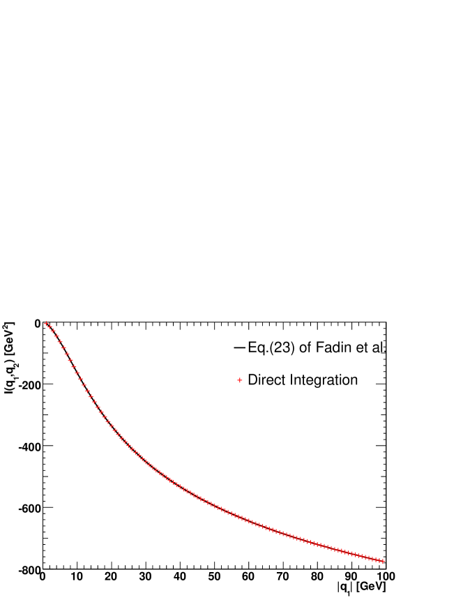
Figure 2: The quantity $I(\mathbf{q}_{1},\mathbf{q}_{2})$ of Eq. (19) for $\mathbf{q}_{2}=(0,15)$ GeV and $\mathbf{q}_{1}$ varying along $(1,0)$ compared between the results obtained in this paper and the corrected results of Ref.[11].

The complete agreement verifies that our implementation of the amplitudes and parametrisation of phase space is correct.

2.2 Regularisation

We now want to regularise the integral in Eq. (15) in order to implement the quark contribution to the fully exclusive Lipatov vertex at NLL. We will start by rewriting[14, 10] the amplitude $A^{\bar{q}q}_{+-}(k_{1},k_{2})$

$$\begin{split}A^{\bar{q}q}_{+-}(k_{1},k_{2})=&-\sqrt{\frac{1-x}{x}}\Bigg{[}\frac{k_{1\perp}^{*}(q_{2\perp}+k_{2\perp})}{\hat{t}}+\frac{x|q_{1\perp}|^{2}k_{1\perp}^{*}k_{2\perp}}{|\Delta_{\perp}|^{2}(|k_{1\perp}-x\Delta_{\perp}|^{2}+x(1-x)|\Delta_{\perp}|^{2})}\\ &-\frac{x(1-x)q_{1\perp}q_{2\perp}^{*}}{\Delta_{\perp}^{*}(k_{1\perp}-x\Delta_{\perp})}+\frac{xq_{1\perp}^{*}q_{2\perp}k_{1\perp}^{*}}{|\Delta_{\perp}|^{2}(k_{1\perp}^{*}-x\Delta_{\perp}^{*})}+\frac{xq_{2\perp}^{*}}{\Delta_{\perp}^{*}}\Bigg{]}\end{split}$$ (20)

with

$$\begin{split}\hat{t}=&-\frac{|k_{1\perp}-xq_{1\perp}|^{2}+x(1-x)|q_{1\perp}|^{2}}{x},\qquad x=\frac{k_{1}^{+}}{k_{1}^{+}+k_{2}^{+}}\\ \hat{s}_{12}&=\frac{\left|k_{1\perp}-x\Delta_{\perp}\right|}{x(1-x)},\qquad\Delta_{\perp}=k_{1\perp}+k_{2\perp}\end{split}$$ (21)

The quark–anti-quark contribution has two divergences: A singularity at $k_{1}^{+}-x\Delta_{\perp}\to 0$ and one at $\Delta_{\perp}^{2}=0$. When constructing the regularised vertex, the first type of singularity is regularised by the corresponding singularity from the one-loop corrections to the one-gluon production, whereas the second type of singularity is regularised by the corresponding one in the gluon trajectory. In the framework of the direct solution to the BFKL evolution, the regularisation of the latter divergence was performed already in Ref.[12, 13]. In the present context we therefore need only to consider $\Delta_{\perp}^{2}\not=0$. In order to implement the exclusive NLL Lipatov vertex, we would need to perform the regularisation of the divergence at $k_{1\perp}-x\Delta_{\perp}\to 0$ using a phase space slicing method. Technically, we will perform the phase space integration by Monte Carlo techniques. If $A^{\bar{q}q}_{+-}(k_{1},k_{2})$ is probed for $k_{1\perp}-x\Delta_{\perp}>\lambda$ with $\lambda$ small (our reported results are stable for variations of $\lambda$ between $10^{-2}$ GeV and $10^{-10}$ GeV), the standard result of Eq. (14) is used. When $k_{1\perp}-x\Delta_{\perp}\leq\lambda$, in addition to the non-divergent pieces we return the average value of the integral of $|A^{\bar{q}q}_{+-,\mathrm{div}}(k_{1},k_{2})|^{2}$ combined with the appropriate term from the one–loop quark contribution to the one-gluon emission vertex, evaluated for $\varepsilon\to 0$.

It turns out that only the square of the two terms in Eq. (20) that have an explicit divergence at $k_{1\perp}\to x\Delta_{\perp}$ lead to a pole in $\varepsilon$. All cross terms integrate to zero when integrated for $k_{1\perp}-x\Delta_{\perp}\leq\lambda$. We therefore find

$$\begin{split}|A^{\bar{q}q}_{+-,\mathrm{div}}(k_{1},k_{2})|^{2}&\to\frac{1-x}{x}\left(\left|\frac{x(1-x)q_{1\perp}q_{2\perp}^{*}}{\Delta_{\perp}^{*}(k_{1\perp}-x\Delta_{\perp})}\right|^{2}+\left|\frac{xq_{1\perp}^{*}q_{2\perp}k_{1\perp}^{*}}{|\Delta_{\perp}|^{2}(k_{1\perp}^{*}-x\Delta_{\perp}^{*})}\right|^{2}\right)\\ &=\frac{1-x}{x}\frac{\mathbf{q}_{1}^{2}\mathbf{q}_{2}^{2}}{\mathbf{\Delta}^{2}(\mathbf{k}_{1}-x\mathbf{\Delta})^{2}}\left(x^{2}(1-x)^{2}+x^{4}\right).\end{split}$$ (22)

Using

$$\mathrm{d}\eta=\frac{\mathrm{d}x}{2x(1-x)}$$ (23)

and the substitution $\mathbf{k}_{1}-x\mathbf{\Delta}\to\mathbf{l}$ together with the following result

$$\int_{|l|=0}^{|l|=\lambda}\frac{\mathrm{d}^{D-2}\mathbf{l}}{l^{2}}=\frac{\pi^{1+\varepsilon}}{\Gamma(1+\varepsilon)}\frac{1}{\varepsilon}(\lambda^{2})^{\varepsilon}$$ (24)

with $D=4+2\varepsilon$, we can obtain the Laurent series in $\varepsilon$ for the relevant phase space integral of each of the contributing terms. The result is

$$\frac{g^{4}\mu^{2\varepsilon}}{\mathbf{\Delta}^{2}\ (2\pi)^{6}}n_{f}N_{c}\frac{\pi^{1+\varepsilon}}{3\ \Gamma(1+\varepsilon)}\frac{1}{\varepsilon}(\lambda^{2})^{\varepsilon}$$ (25)

The generated divergence cancels with the divergent part of the one–loop quark contribution to the one-gluon emission vertex in Eq. (11).

3 Discussion

Having thus constructed the regularised quark contribution, we can calculate the contribution to the BFKL kernel as in Eq. (15) (remembering that also the divergent contribution from the virtual corrections are taken into account). The Monte Carlo method allow us to study directly the differential distribution in any variable. Of particular interest is the distribution in the energy of the Reggeon-Reggeon collision. The LL contribution come from the emission of a single gluon of energy $|\mathbf{q}_{1}-\mathbf{q}_{2}|$. However, when the NLL corrections are calculated as in Eq. (15), contributions arise from all energies above this scale. In Fig. 3 we have plotted the distribution in the energy of the Reggeon-Reggeon collisions contributing to the NLL corrections to the LL result. We have chosen $\mathbf{q}_{1}$ and $\mathbf{q}_{2}$ to be perpendicular, with $|\mathbf{q}_{1}|=|\mathbf{q}_{2}|=20$ GeV, however the findings have general validity. The average energy of the Reggeon-Reggeon collisions included in the NLL corrections calculated according to Eq. (15) is $\approx 40\%$ larger than the energy in the LL setup (for all angles and for an arbitrary value of $|\mathbf{q}_{1}|=|\mathbf{q}_{2}|$). Furthermore, the average rapidity separation between the quark and the anti-quark is $\approx.56$ units of rapidity. Often, the contribution supposed to described the radiative corrections to a single gluon emission would be described as a two-jet configuration! All the quark–anti-quark configurations included in the integrations of Eq. (15) must be included in the evolution to obtain overall NLL accuracy. But assigning them all to a single transverse scale will potentially greatly exaggerate the impact of these NLL corrections on the evolution.

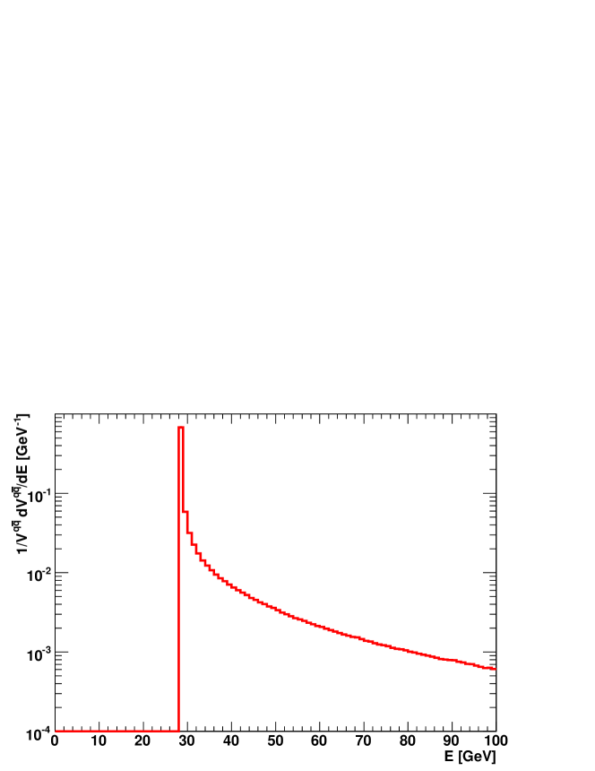
Figure 3: The energy distribution of the contribution to the NLL corrections to a Reggeon-Reggeon collision of $\sqrt{2}\cdot 20$ GeV in the standard approach.

However, this is a problem that cannot be resolved as long as only transverse degrees of freedom are considered in the governing BFKL equation. We therefore propose a framework which will perform the BFKL evolution fully differentially in the momenta of all emitted particles, i.e. not only using the fully differential BFKL equation[3, 13, 12]

$$\frac{\partial}{\partial y_{j}}\ \frac{\partial}{\partial k_{j\perp}}\ f(\mathbf{q}_{a},\{k_{i\perp},y_{i}\},\mathbf{q}_{b},y)=K\left(\mathbf{q}_{a}+\sum_{i=1}^{j-1}k_{i\perp},\mathbf{q}_{a}+\sum_{i=1}^{j}k_{i\perp}\right)\ f(\mathbf{q}_{a},\{k_{i\perp},y_{i}\},\mathbf{q}_{b},y),$$ (26)

but also keeping the NLL corrections fully exclusive as detailed in this study for the quark contributions. This will ensure not only the conservation of all components of the momentum vector, but also that for a given set of Reggeon momenta, only the relevant NLL corrections are included. The result of such evolution would be in complete agreement with the description of the Reggeisation of $t$-channel gluon amplitudes according to Ref.[15], when also here the NLL vertices are kept exclusive. Of course the result of the standard BFKL formalism can be obtained by suitable phase space integrations and ignorance of the conservation of longitudinal momentum.

The large spread in energies of the contributions to the NLL corrections will have sizeable effects in a realistic application of the BFKL framework. In the application of the BFKL framework to the description of the small-$x$ behaviour of partons, the calculated NLL corrections to the kernel cannot be ascribed to a single value of $x$. And in the emerging framework of applying the BFKL evolution in the description of the production of multiple hard jets, the NLL corrections would be weighted with different pdf-factors, according to their relevant contribution to the centre of mass energy. This effect will change the impact of the NLL corrections, and could further reduce their importance.

4 Conclusions

We have presented a new calculation of the quark contribution to the NLL corrections to the BFKL kernel, based on an explicit Monte Carlo integration of the produced particles. We have demonstrated that in the standard calculation of the NLL BFKL kernel, the NLL corrections arise from Reggeon-Reggeon energies far higher than that which is probed at LL. This exaggerates the apparent effect of the NLL corrections.

We have presented a method which will assign the NLL corrections to the appropriate LL contributions. We are looking forward to reporting on the gluon contribution to the NLL corrections, and on the implementation of the new framework in the prediction for multi-jet events at the LHC.

Acknowledgements

I would like to thank Robert S. Thorne for discussions leading to the localisation of a misprint in Ref.[11]. I thank Einan Gardi, Robert S. Thorne and Bryan R. Webber for many stimulating discussions.

References

• [1] V. S. Fadin and L. N. Lipatov, BFKL pomeron in the next-to-leading approximation, Phys. Lett. B429 (1998) 127–134, [hep-ph/9802290].
• [2] M. Ciafaloni and G. Camici, Energy scale(s) and next-to-leading BFKL equation, Phys. Lett. B430 (1998) 349–354, [hep-ph/9803389].
• [3] J. R. Andersen, On the role of NLL corrections and energy conservation in the high energy evolution of QCD, Phys. Lett. B639 (2006) 290–293, [hep-ph/0602182].
• [4] V. S. Fadin and L. N. Lipatov, Radiative corrections to QCD scattering amplitudes in a multi-Regge kinematics, Nucl. Phys. B406 (1993) 259–292.
• [5] V. S. Fadin, R. Fiore, and A. Quartarolo, Radiative corrections to quark quark reggeon vertex in QCD, Phys. Rev. D50 (1994) 2265–2276, [hep-ph/9310252].
• [6] V. S. Fadin, R. Fiore, and M. I. Kotsky, Gribov’s theorem on soft emission and the Reggeon-Reggeon-gluon vertex at small transverse momentum, Phys. Lett. B389 (1996) 737–741, [hep-ph/9608229].
• [7] V. Del Duca and C. R. Schmidt, Virtual next-to-leading corrections to the Lipatov vertex, Phys. Rev. D59 (1999) 074004, [hep-ph/9810215].
• [8] V. S. Fadin, BFKL news, hep-ph/9807528.
• [9] L. N. Lipatov, Gauge invariant effective action for high-energy processes in QCD, Nucl. Phys. B452 (1995) 369–400, [hep-ph/9502308].
• [10] V. Del Duca, Quark-antiquark contribution to the multigluon amplitudes in the helicity formalism, Phys. Rev. D54 (1996) 4474–4482, [hep-ph/9604250].
• [11] V. S. Fadin, R. Fiore, A. Flachi, and M. I. Kotsky, Quark-antiquark contribution to the BFKL kernel, Phys. Lett. B422 (1998) 287–293, [hep-ph/9711427].
• [12] J. R. Andersen and A. Sabio Vera, Solving the BFKL equation in the next-to-leading approximation, Phys. Lett. B567 (2003) 116–124, [hep-ph/0305236].
• [13] J. R. Andersen and A. Sabio Vera, The gluon Green’s function in the BFKL approach at next-to-leading logarithmic accuracy, Nucl. Phys. B679 (2004) 345–362, [hep-ph/0309331].
• [14] V. S. Fadin and L. N. Lipatov, Next-to-leading corrections to the BFKL equation from the gluon and quark production, Nucl. Phys. B477 (1996) 767–808, [hep-ph/9602287].
• [15] V. S. Fadin, R. Fiore, M. G. Kozlov, and A. V. Reznichenko, Proof of the multi-Regge form of QCD amplitudes with gluon exchanges in the NLA, Phys. Lett. B639 (2006) 74–81, [hep-ph/0602006].