Quantum Gravity Effects in Black Holes at the LHC

Abstract

We study possible back-reaction and quantum gravity effects in the evaporation of black holes which could be produced at the LHC through a modification of the Hawking emission. The corrections are phenomenologically taken into account by employing a modified relation between the black hole mass and temperature. The usual assumption that black holes explode around $1\,$TeV is also released, and the evaporation process is extended to (possibly much) smaller final masses. We show that these effects could be observable for black holes produced with a relatively large mass and should therefore be taken into account when simulating micro-black hole events for the experiments planned at the LHC.

1 Introduction

One of the most exciting feature of models with large extra dimensions [1, 2] is the fact that the fundamental scale of gravity $M_{\rm G}$ could be as low as the electro-weak scale ($M_{\rm G}\simeq 1$ TeV) and micro-black holes  may therefore be produced in our accelerators [3, 4, 5, 6, 7]. Once a black hole has formed (and after possible transients) the Hawking radiation [11] is expected to set off. The most common description of this effect is based on the canonical  Planckian distribution for the emitted particles and on the consequence that the life-time of micro-black holes is so short that the decay can be viewed as sudden [7]. This standard picture has already been implemented in several numerical codes [18, 19, 20, 21] which let the black hole decay down to an arbitrary mass $M_{\rm f}$ of order $M_{\rm G}$ via the Hawking law and then explode into a small number of decay products. By running these numerical codes, one mostly aims at extracting information that will allow us to identify micro-black hole events in the planned experiments based, for example, on some experimental features of the decay products [22] or on some particular signatures of the decay [23].

We would like to stress here that the issue of the end of the black hole evaporation remains an open question (see, e.g., Refs. [24, 25, 26]) because we do not yet have a reliable theory of quantum gravity and, most of all, no experimental data from the quantum gravity regime. The singular behavior of the Hawking temperature as the black hole mass decreases to zero can in fact be simply viewed as a sign of the lack of predictability of perturbative approaches. Therefore, although the very detection of these objects would already be evidence that $M_{\rm G}$ is not the Planck energy (about $10^{19}\,$GeV) and that extra dimensions may indeed exist, observing the late stages of black hole evaporation (when the black hole mass $M\sim M_{\rm G}$) could provide us with the kind of data we need to finally build the theory of quantum gravity. On a purely experimental side, this is also an important issue, since it corresponds to determine whether some features usually associated with the black hole decay are sensitive to the assumptions made about the late stages of the evaporation. This is equivalent to asking whether deviations from the Hawking law, induced by an underlying and still unknown theory of quantum gravity, can actually be detected. In some sense, this is analogous to the problem of trans-Planckian modes in cosmology, where one can ask whether the still unknown physics at Planck scales, which is certainly important in the early stages of the Universe, can affect the CMB spectrum we observe now.

As we mentioned above, the ignorance of the late stages of the black hole evaporation is bypassed in the numerical codes by letting the micro-black hole decay into a few standard model particles as an arbitrary lower mass is reached (the possibility of ending the evaporation by leaving a stable remnant has also been recently considered [27, 28]). The purpose of this report is precisely to study if modifications of this standard description of the evaporation which could occur as the black hole mass becomes smaller than some arbitrary scale ($M\lesssim M_{\rm G}$) can produce experimentally detectable features, although we shall not consider a specific experimental setup and leave for future developments the task of including the detector’s sensitivity and geometry. From another perspective, one can also view this preliminary analysis as an estimate of the systematic errors to be associated with the results already appeared on this subject that usually rely on the standard picture we described above.

For this purpose, we have developed several modifications to the Monte Carlo code CHARYBDIS [18] which we shall describe in Section 3 (see also Ref. [15]). We shall then report some interesting and perhaps unexpected (preliminary) results from a few test runs in Section 4. We shall use units with $c=\hbar=1$ and the Boltzmann constant $k_{\rm B}=1$.

2 Black hole evaporation

No-hair theorems of General Relativity guarantee that a black hole is characterized by its mass, charges and angular momentum only. The one parameter characterizing an uncharged, non-rotating black hole is thus its mass $M$. On considering solutions to the Einstein equations (or applying Gauss’ theorem) in $4+d$ dimensions, one can then derive the following relation between the mass and the horizon radius,

$$R_{\rm H}=\frac{1}{\sqrt{\pi}\,M_{\rm G}}\,\left(\frac{M}{M_{\rm G}}\right)^{\frac{1}{d+1}}\left(\frac{8\,\Gamma\left(\frac{d+3}{2}\right)}{d+2}\right)^{\frac{1}{d+1}}\ ,$$ (2.1)

where $\Gamma$ is the usual Gamma function, and the temperature associated with the horizon is given by

$$T_{\rm H}=\frac{d+1}{4\,\pi\,R_{\rm H}}\ .$$ (2.2)

Once formed, the black hole begins to evolve. In the standard picture the evaporation process can be divided into three characteristic stages [4]:

1. Balding phase: the black hole radiates away the multipole moments it has inherited from the initial configuration, and settles down in a hairless state. A certain fraction of the initial mass will also be lost in gravitational radiation.

2. Evaporation phase: it starts with a spin down phase in which the Hawking radiation [11] carries away the angular momentum, after which it proceeds with the emission of thermally distributed quanta until the black hole reaches the Planck mass (replaced by the fundamental scale $M_{\rm G}$ in the models we are considering here). The radiation spectrum contains all the Standard Model particles, which are emitted on our brane, as well as gravitons, which are also emitted into the extra dimensions. It is in fact expected that most of the initial energy is emitted during this phase into Standard Model particles [6] (although this conclusion is still being debated, see e.g., Ref. [29]).

3. Planck phase: once the black hole has reached a mass close to the effective Planck scale $M_{\rm G}$, it falls into the regime of quantum gravity and predictions become increasingly difficult. It is generally assumed that the black hole will either completely decay into some last few Standard Model particles or a stable remnant be left which carries away the remaining energy [27].

In our approach we will consider possible modifications to the second and third phases. On the one hand, we will allow a modified Hawking phase by employing a different relation between the horizon radius and the temperature. The necessity of such a modification, suggested by the fact that the Hawking temperature diverges as the mass of the black hole goes to zero, has been discussed in several papers, e.g., Refs. [30, 31]. We will follow a phenomenological approach to this issue and model a general class of modifications by making use of the form given in Eq. (3.2) below. On the other hand, we will look at the possibility that the evaporation may not end at the fundamental scale $M_{\rm G}$ ($\sim 1\,$TeV) but proceeds further until a lower (arbitrary) mass $M_{\rm f}$ has been reached.

3 Quantum Gravity and Monte Carlo code

Several Monte Carlo codes which simulate the production and decay of micro-black holes are now available (see, e.g. Refs. [18, 19, 20]). We have found it convenient to implement our modifications into CHARYBDIS [18].

In order to let the black hole evaporate below the electro-weak scale $M_{\rm EW}$, at which the Standard Model particles acquire their mass, one needs to treat the mass of the emitted particles properly. In the original code, the phase space was taken to be that of massless particles since the mass of the black hole $M\gtrsim M_{\rm f}$ and $M_{\rm f}>M_{G}>M_{\rm EW}$. However, we also want to consider the possibility that the black hole decays to lower masses, that is $M_{\rm f}\ll M_{G}$. We therefore use the phase space measure in the Planckian number density for the emitted particles given by

$$N_{m}(\vec{k})=\frac{d^{3}k}{e^{\omega/T}\pm 1}\ ,$$ (3.1)

where $T$ denotes the black hole temperature, $m$ the particle mass, $\vec{k}$ the particle 3-momentum and $\omega=\sqrt{k^{2}+m^{2}}$. Moreover, since $N_{m}$ depends on $m$ and not just on the statistics, one can no more assume (as in CHARYBDIS) a fixed ratio of production for fermions versus bosons but proper particle multiplicity must be used when generating particle types randomly. We used the multiplicities predicted by the Standard Model [32] and modified the code accordingly.

$T$       $T$

$M$                                                              $M$

Figure 1: Black hole temperature (in GeV) as a function of the black hole mass (in GeV). Left panel: comparison between the Hawking law $T_{\rm H}$ (solid line) and $T_{1}$ from Eq. (3.3) for $\ell=10^{-3}\,$GeV^-1, $\alpha=5$, $n=5$ (dashed line) and $\ell=10^{-3}\,$GeV^-1, $\alpha=5$, $n=1$ (dotted line). Right panel: $T_{\rm H}$ (solid line) compared to $T_{2}$ from Eq. (3.4) with $\ell=1.14\cdot 10^{-4}\,$GeV^-1, $n_{1}=1$, $n_{2}=1$ (dotted line).

In order to include possible quantum gravity effects, we employ modified expressions for the temperature $T=T_{i}$ of the form

$$T_{i}=F_{i}\,T_{\rm H}\ ,$$ (3.2)

in which, in order to cover results in the existing literature (for a partial list of approaches to the problem, see Refs. [12, 14, 16, 17, 31]) we shall consider the functional forms

$$F_{1}(\ell,\alpha,n)=\frac{R_{\rm H}^{n}}{R_{\rm H}^{n}+\alpha\,\ell^{n}}$$ (3.3)

and

$$F_{2}(\ell,n_{1},n_{2})=\left[1-\left(\frac{\ell}{R_{H}}\right)^{n_{1}}\right]^{n_{2}}\ ,$$ (3.4)

where $\ell$, $\alpha$, $n$, $n_{1}$, and $n_{2}$ are parameters that can be adjusted (see below). Note that $F_{1}$ leads to a vanishing temperature for vanishing black hole mass (horizon radius) whereas with $F_{2}$ the temperature vanishes at finite $M$ when $R_{\rm H}=\ell$ [31] (such a remnant was also considered in Ref. [27]). Specific examples which will be used throughout the paper are shown in Fig. 1 together with the standard Hawking law (2.2).

A list of some adjustable parameters in the code is given in Table 1. The initial black hole mass $M_{0}$ can be either fixed (to within the maximum centre mass energy expected at the LHC) or generated according to the partonic cross section. In the simulations we present here, we shall take a total centre mass energy of $14\,$TeV and mostly focus on the the case of $M_{0}=10\,$TeV (with $M_{0}=2\,$TeV taken for comparison ). At the end point of the decay, the black hole explodes in a selectable number $N_{\rm f}$ of fragments when $M\lesssim M_{\rm f}$. We shall use $N_{\rm f}=2$ and set the total number of space-time dimensions equal to 6. We shall also set the grey-body factors equal to 1 for all kinds of particles. This approximation is certainly restrictive and calls for a more refined analysis. However, we note that in the standard picture the use of more accurate grey-body factors alters the final results only by a small amount and we thus feel that our modified code can be regarded as a good tool to study qualitative features related to the late stages of the evaporation. A substantial modification of CHARYBDIS will likely be necessary if one wants to obtain more accurate predictions about, for example, the actual modification of the Hawking emission.

$M_{0}$ Initial black hole mass $1-14$ TeV; random $M_{\rm f}$ Minimum black hole mass $1-1000$ GeV $N_{\rm f}$ number of final fragments $2-6$ $d$ number of extra dimensions $1-5$ $F_{i}$ modified temperature $1$ (no modification), $F_{1}$, $F_{2}$

Table 1: Parameters that can be adjusted in our Monte Carlo generator and their ranges. For each modified temperature, one can also set the corresponding parameters as described in the text.

4 Simulation Results

The standard CHARYBDIS generator simulates the evaporation of a micro-black hole according to Hawking’s law until the black hole mass $M$ reaches the minimum value $M_{\rm f}$ which is assumed equal to the fundamental scale of gravity $M_{\rm G}$ in a given model of extra dimensions (e.g., at $1\,$TeV). The black hole subsequently decays into a few bodies ($N_{\rm f}=1,\ldots,6$) simply according to phase space. As described in the previous section, in our modified code, we implemented ways to extend the evaporation to a mass $M_{\rm f}$ well below the fundamental scale (e.g., down to $1\,$GeV).

In the following, we shall compare the outputs of the standard and modified generators from a phenomenological point of view. In particular, we shall consider the output of the standard code with $M_{\rm f}=1\,$TeV (and $M_{\rm f}=1\,$GeV for completeness) as reference. The results for the modified temperature $T_{1}$ were obtained with $M_{\rm f}=1\,$GeV and the parameters $\ell=10^{-3}\,$GeV^-1, $\alpha=5$, $n=5$ (see Eq. (3.3)) and those for the temperature $T_{2}$ with $\ell=1.14\cdot 10^{-4}\,$GeV^-1, $n_{1}=1$, $n_{2}=1$ (see Eq. (3.4)). Note that the latter choice of parameters also corresponds to a final mass of the black hole equal to $M_{\rm f}\simeq 1\,$GeV at which the temperature $T_{2}=0$. These cases are the same that were shown previously in Fig. 1.

4.1 Primary Emission

Figure 2: Left panel: abundance of Standard Model particles produced during the evaporation of $10\,$TeV black holes before hadronization, for a run of 10000 events with the temperature $T_{1}$ (solid histogram) and with the standard CHARYBDIS generator (dashed histogram). The fundamental scale of gravity is set to $1\,$TeV, temperature parameters are the same as in Fig. 1 and number of extra dimensions $d=2$. Right panel: energy distribution of the emitted particles obtained from $T_{1}$ (solid histogram), including only particles emitted when the black hole has a mass exceeding $1\,$TeV (dashed histogram), and with the standard CHARYBDIS generator (dotted histogram).

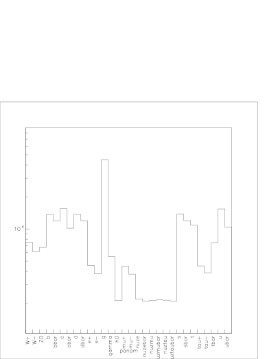
Figure 3: Abundance of Standard Model particles produced during the evaporation of $10\,$TeV black holes for a run of 10000 events before hadronization. Upper graphs: standard CHARYBDIS generator with $M_{\rm f}=1\,$TeV (left panel) and $M_{\rm f}=1\,$GeV (right panel). Lower graphs: modified code with the temperature $T_{1}$ (left panel) and $T_{2}$ (right panel) and $M_{\rm f}=1\,$GeV.

Figure 4: Energy spectrum of particles produced during the evaporation of $10\,$TeV black holes for a run of 10000 events before hadronization: standard CHARYBDIS generator with $M_{\rm f}=1\,$TeV (dotted line) and $M_{\rm f}=1\,$GeV (dashed line), modified code with the temperature $T_{1}$ (solid line) and $T_{2}$ (indistiguishable from the dashed).

Let us first examine the “primary” black hole emission, namely the particles produced by direct black hole evaporation before parton evolution and hadronization are taken into account. As we mentioned before, we set the mass for the final decay of the black hole at $M_{\rm f}=1\,$TeV in the standard case and at $M_{\rm f}=1\,$GeV for the modified temperatures.

A comparison of the relative abundance of the Standard Model particles produced by the black hole evaporation with the Hawking temperature and the modified temperature $T_{1}$ from Eq. (3.3) is shown in the left panel of Fig. 2. For the temperature $T_{1}$, this plot clearly shows a much larger multiplicity of isotropically emitted light particles (i.e., photons and neutrinos as well as electrons and muons). In the right panel of Fig. 2, we also show the energy distribution of all the emitted particles. The modified law dramatically changes the spectrum at low energy (there are about three orders of magnitude more particles with energy below $100\,$GeV than in the standard case), leaving the spectrum at large energy moderately affected (by just about one order of magnitude). Note that the low energy distribution of particles emitted when the black hole mass $M>1\,$TeV follows closely the standard curve but that there are already missing particles in the high energy tail (above $1\,$TeV).

For completeness, in Fig. 3, we show the particle abundance obtained with the standard CHARYBDIS generator if we set $M_{\rm f}=1\,$GeV and compare it with the results from the modified code for the two different temperatures $T_{1}$ and $T_{2}$ and $M_{\rm f}=1\,$GeV. It then appears that the temperature $T_{1}$ leads to a number of light particles significantly larger than the other three cases. The temperature $T_{2}$ instead produces about the same amount of light particles as the standard Hawking temperature provided the evaporation is extended down to $M_{\rm f}=1\,$GeV. The corresponding energy distributions are given in Fig. 4, from which one concludes that the number of high energy particles produced with $T_{2}$ is also closer to the standard case with $M_{\rm f}=1\,$GeV. To conclude, if one just considers the above data, there is no visible difference in the primary emission between $T_{2}$ and the Hawking temperature provided both are extended to a minimum black hole mass of $1\,$GeV, whereas the spectrum generated with $T_{1}$ still shows appreciable differences.

These behaviors can be understood in the following way: since the temperature $T_{1}$ tends to zero for $M=0$, we do expect a continuous emission of increasingly softer particles until the black hole evaporates completely (i.e., it reaches the minimum value $M_{\rm f}=1\,$GeV). Moreover, once the black hole mass has decreased below the threshold for producing a given massive particle, such a particle can no longer be emitted. Hence one also expects that the production of the heavier particles (i.e., massive gauge bosons and top quarks) be scarcely affected, while the emission of soft low mass (or massless) particles should be largely enhanced. For the temperature $T_{2}$, the situation is similar except that its functional form follows the Hawking law more closely and the distribution of particles more closely resembles the standard case provided one allows the black hole to evaporate down to the same mass at which $T_{2}$ vanishes ($1\,$GeV in our samples).

4.2 Final Output

Figure 5: Final abundance of Standard Model particles produced during the evaporation of $10\,$TeV black holes for a run of 10000 events. Upper graphs: standard CHARYBDIS generator with $M_{\rm f}=1\,$TeV (left panel) and $M_{\rm f}=1\,$GeV (right panel). Lower graphs: modified code with the temperature $T_{1}$ (left panel) and $T_{2}$ (right panel).

Figure 6: Final abundance of Standard Model particles produced during the evaporation of $2\,$TeV black holes for a run of 10000 events. Upper graphs: standard CHARYBDIS generator with $M_{\rm f}=1\,$GeV Lower graphs: modified code with the temperature $T_{1}$ (left panel) and $T_{2}$ (right panel).

Figure 7: Statistical distribution of the sum of particle transverse momenta including only particles with transverse momentum higher than $30\,$GeV for 10000 events for the decay of $10\,$TeV black holes (left graph) and of $2\,$TeV black holes (right graph): standard CHARYBDIS generator with $M_{\rm f}=1\,$TeV (pointed line) and $M_{\rm f}=1\,$GeV (dashed line), modified code with the temperature $T_{1}$ (solid line) and $T_{2}$ (indistinguishable from dashed line).

Figure 8: Sum of the muon transverse momenta in the range $0-10\,$GeV including only particles with transverse momentum higher than $30\,$GeV for the decay of $10\,$TeV black holes. Left panel: standard CHARYBDIS generator with $M_{\rm f}=1\,$TeV. Right panel: modified code with the temperature $T_{1}$ for $M_{\rm f}=1\,$GeV.

The primary output includes quarks and gluons that cannot be detected. We therefore used Pythia [33] to model the parton evolution and hadronization of quarks and gluons emitted during the evaporation (or not participating to the black hole events). This produced the final aspect of the events as would be seen by a detector at the LHC.

In Fig. 5, we show the final particle abundance for the standard Hawking temperature and $M_{\rm f}=1\,$TeV or $M_{\rm f}=1\,$GeV and the modified temperatures $T_{1}$ and $T_{2}$ with $M_{\rm f}=1\,$GeV. The first thing one notes is that the standard Hawking temperature for both $M_{\rm f}=1\,$TeV or $M_{\rm f}=1\,$GeV and the temperature $T_{2}$ now produce very similar numbers of particles. In contrast to the primary output, the temperature $T_{1}$ now produces a number of photons and pions smaller than the other cases. The number of muons and electrons in the final state is however still higher (by a factor around 2) for $T_{1}$ with respect to all other cases. In the case of a black hole with initial mass of $2\,$TeV, Fig. 6 shows no evident difference in the number of produced particles for the four cases previously discussed.

Another remarking feature of the events produced with the temperature $T_{1}$ is that the distribution of the sum of transverse momenta for particles with transverse momentum higher than $30\,$GeV is peaked around a larger value (about $5\,$TeV) compared to the results for the other three cases, as shown in the left graph of Fig. 7 (in the right graph, the analogue distributions for $M_{0}=2\,$TeV are showed). If one counts all particles, however, such distributions show no appreciable difference. Finally, we remark that the distribution for the sum of the muon transverse momenta for the temperature $T_{1}$ does not show a peak around zero, contrary to all other cases. The same feature appears if one only counts muons with transverse momentum over $30\,$GeV see Fig. 8.

5 Conclusions

We have considered possible modifications to the standard picture of the decay of micro-black holes that might be produce at the LHC. Inspired by the microcanonical description of the Hawking evaporation and other theoretical approaches in the literature, we have studied modified statistical laws for the emitted particles described by different mass-dependent temperatures $T_{1}$ and $T_{2}$ which have a regular behavior for vanishing black hole mass. We have also required that energy be conserved all the way to the end of the evaporation at a scale $M_{\rm f}\ll M_{\rm G}$. We have not explicitly considered the case in which black holes leave stable remnants, since that has already been reported in Ref. [27]. Further, our temperature $T_{2}$ corresponds to a zero-temperature remnant of finite mass which suddenly decays in a few particles.

The numerical simulations we have run so far suggest that this kind of modifications, if present, might have significant and testable effects for black holes produced with a (relatively) large initial mass (of the order of ten times the fundamental scale of gravity $M_{\rm G}$). On assuming that $M_{\rm G}=1\,$TeV, the LHC at full luminosity is expected to produce around three $10\,$TeV black holes per day [4]. Such a production rate, although smaller than the $1\,$Hz for $5\,$TeV black holes (and even larger for $2\,$TeV black holes) is however large enough to collect sufficient data to compare with the results we have presented here and their signature should also be easier to identify than that for lighter black holes. For example, one expects to see differences in the number of particles produced and in their total transverse momentum. It is therefore important to take into account these possibilities in any detailed simulation of the evaporation process whose outputs will have to be confronted with forthcoming data.

References

- [1] N. Arkani-Hamed, S. Dimopoulos and G. Dvali, Phys. Lett. B 429, 263 (1998); Phys. Rev. D 59, 0806004 (1999); I. Antoniadis, N. Arkani-Hamed, S. Dimopoulos and G. Dvali, Phys. Lett. B 436, 257 (1998).
- [2] L. Randall and R. Sundrum, Phys. Rev. Lett. 83, 4690 (1999); Phys. Rev. Lett. 83, 3370 (1999).
- [3] T. Banks and W. Fishler, hep-th/9906038;
- [4] S.B. Giddings and S. Thomas, Phys. Rev. D 65, 056010 (2002)
- [5] P.C. Argyres, S. Dimopoulos and J. March-Russell, Phys. Lett. B 441, 96 (1998);
- [6] R. Emparan, G.T. Horowitz and R.C. Myers, Phys. Rev. Lett. 85, 499 (2000).
- [7] S. Dimopoulos and G. Landsberg, Phys. Rev. Lett. 87, 161602 (2001).
- [8] L.A. Anchordoqui, H. Goldberg and A.D. Shapere, Phys. Rev. D 66 (2002) 024033.
- [9] A. Chamblin, S. Hawking and H.S. Reall, Phys. Rev. D 61, 0605007 (2000); R. Casadio and L. Mazzacurati, Mod. Phys. Lett. A 18, 651 (2003); R. Casadio, A. Fabbri and L. Mazzacurati, Phys. Rev. D 65, 084040 (2002); R. Casadio, Phys. Rev. D 69, 084025 (2004).
- [10] M. Cavaglia, Int. J. Mod. Phys. A 18, 1843 (2003); P. Kanti, Int. J. Mod. Phys. A 19, 4899 (2004).
- [11] S.W. Hawking, Nature 248, 30 (1974); Comm. Math. Phys. 43, 199 (1975).
- [12] R. Casadio, B. Harms and Y. Leblanc, Phys. Rev. D 57, 1309 (1998); R. Casadio and B. Harms, Phys. Rev. D 58, 044014 (1998) and Mod. Phys. Lett. A14, 1089 (1999).
- [13] R. Casadio and B. Harms, Phys. Rev. D 64, 024016 (2001).
- [14] S. Hossenfelder, S. Hofmann, M. Bleicher and H. Stoecker, Phys. Rev. D 66, 101502 (2002).
- [15] G. L. Alberghi, R. Casadio, D. Galli, D. Gregori, A. Tronconi and V. Vagnoni, “Probing quantum gravity effects in black holes at LHC,” hep-ph/0601243.
- [16] T. G. Rizzo, hep-ph/0510420 and Class. Quant. Grav. 23, 4263 (2006); R. Casadio and B. Harms, Phys. Lett. B 487, 209 (2000); R. Casadio, Annals Phys. 307, 195 (2003); S.D.H. Hsu, Phys. Lett. B 555, 92 (2003).
- [17] R. Casadio and B. Harms, Int. J. Mod. Phys. A 17, 4635 (2002).
- [18] C. M. Harris, P. Richardson and B.R. Webber, JHEP 0308, 033 (2003).
- [19] S. Dimopoulos and G. Landsberg, Black hole production at future colliders, in Proc. of the APS/DPF/DPB Summer Study on the Future of Particle Physics (Snowmass 2001), edited by N. Graf, eConf C010630, P321 (2001).
- [20] E.J. Ahn and M. Cavaglia, Phys. Rev. D 73, 042002 (2006).
- [21] M. Cavaglia, R. Godang, L. Cremaldi and D. Summers, “Catfish: A Monte Carlo simulator for black holes at the LHC,” hep-ph/0609001.
- [22] J.L. Hewett, B. Lillie and T.G. Rizzo, Phys. Rev. Lett. 95, 261603 (2005).
- [23] T.J. Humanic, B. Koch and H. Stocker, hep-ph/0607097.
- [24] G. Landsberg, J. Phys. G 32, R337 (2006).
- [25] C.M. Harris, M.J. Palmer, M.A. Parker, P. Richardson, A. Sabetfakhri and B. R. Webber, JHEP 0505, 053 (2005).
- [26] A. Casanova and E. Spallucci, Class. Quant. Grav. 23, R45 (2006).
- [27] B. Koch, M. Bleicher and S. Hossenfelder, JHEP 0510, 053 (2005).
- [28] S. Hossenfelder, Nucl. Phys. A 774, 865 (2006).
- [29] V. Cardoso, M. Cavaglia and L. Gualtieri, JHEP 0602, 021 (2006); V.P. Frolov and D. Stojkovic, Phys. Rev. Lett. 89, 151302 (2002) D. Stojkovic, Phys. Rev. Lett. 94, 011603 (2005).
- [30] R. Balbinot, Phys. Rev. D 33, 1611 (1986); A. Fabbri, D.J. Navarro and J. Navarro-Salas, Gen. Rel. Grav. 33, 2119 (2001); A.V. Frolov, K.R. Kristjansson and L. Thorlacius, Phys. Rev. D 72, 021501 (2005); L. Susskind and L. Thorlacius, Nucl. Phys. B 382, 123 (1992); K. Diba and D. A. Lowe, Phys. Rev. D 65, 024018 (2002); G.L. Alberghi, E. Caceres, K. Goldstein and D.A. Lowe, Phys. Lett. B 520, 361 (2001).
- [31] P. Nicolini, A. Smailagic and E. Spallucci, Phys. Lett. B 632, 547 (2006); T. G. Rizzo, hep-ph/0606051 and hep-ph/0510420.
- [32] S. Eidelman et al. [Particle Data Group], Phys. Lett. B 592, 1 (2004).
- [33] T. Sjostrand, S. Mrenna and P. Skands, JHEP 0605, 026 (2006).