Abstract

O(N) linear $\sigma$ model is solvable in the large $N$ limit and hence provides a useful theoretical laboratory to test various unitarization approximations. We find that the large $N_{c}$ limit and the $m_{\sigma}\to\infty$ limit do not commute. In order to get the correct large $N_{c}$ spectrum one has to firstly take the large $N_{c}$ limit. We argue that the $f_{0}(600)$ meson may not be described as generated dynamically. On the contrary, it is most appropriately described at the same level as the pions, i.e, both appear explicitly in the effective lagrangian. Actually it is very likely the $\sigma$ meson responsible for the spontaneous chiral symmetry breaking in a lagrangian with linearly realized chiral symmetry.

There have been remarkable progresses in recent years in the field of low energy strong interaction physics. In the I=0, J=0 channel of $\pi\pi$ scatterings, it is demonstrated that the $f_{0}(600)$ (or $\sigma$) meson is crucial to adjust chiral perturbation theory to experiments [1], and in fact, the $f_{0}(600)$ meson provides the dominant contribution to the phase shift at low energies. The Roy type equation analyses [2] clearly indicate the existence of a light and broad $S$ matrix pole in the $IJ=00$ channel of $\pi\pi$ elastic scattering amplitude, and also in the I=1/2, J=0 channel $\pi K$ scattering amplitude ($K^{*}(800)$ or $\kappa$) [3]. The dispersive analyses of Refs. [4, 5, 6], firmly demonstrate the existence of the $\sigma$ and the $\kappa$ resonances as well. All the results on the pole positions based on dispersion techniques agree with each other rather well convincingly, within error bars – hence, in the authors’ opinion, settling down the long debate on whether there exist such light and broad resonances. The $\sigma$ meson can also be understood in other approaches. For example, using Dyson–Schwinger equations, in Ref. [7] the mass and even the large width of the $\sigma$ meson can be determined rather well.

Having firmly established the existence of sigma and kappa, the next question would be what these resonances are. There exists a long list of references with quite different opinions. For example, there are attempts to explain these light and broad resonances in linear sigma models at hadron level [8] or at quark level [9]. Interestingly, it was observed that poles corresponding to these lightest scalar resonances can be found in the unitarized amplitudes calculated using chiral perturbation theory, i.e., not having to include the scalars explicitly in the effective lagrangian. Hence the lightest scalars are considered as ‘dynamically generated’ [10]. Unlike a typical resonance, for example, the $\rho(770)$ meson, it is found that the $\sigma$ and $\kappa$ resonance poles move to infinity on the complex $s$ plane in the large $N_{c}$ limit [11]. This different $N_{c}$ behavior is hence believed to be an evidence to support that the $\sigma$ and $\kappa$ are generated dynamically. This aim of this paper is to examine the latter approach closely and try to clarify the meaning of ‘dynamically generated’ resonance.

The idea that a particle can be generated dynamically is not new. Basdevant and Lee have succeeded in generating a dynamical $\rho$ resonance from the renormalizable linear sigma model [12]. On the other side, Basdevant and Zinn-Justin studied the massive Yang-Mills lagrangian in which the $\rho$ meson acts as the massive gauge boson. Through a proper unitarization procedure, they generate in $d$ wave the $f_{2}(1270)$ resonance and a broad $s$ wave $\sigma$ resonance [13]. These activities are closely connected to the old concept of bootstrap duality: in one lagrangian model, a particle may be called elementary (i.e., exhibits itself explicitly in the lagrangian), others are called dynamical (i.e., only show up as $S$ matrix poles but not included in the lagrangian); whereas in other lagrangian models, the particle’s role as ‘elementary’ or ‘dynamical’ can be just reversed.

The idea of bootstrap duality is very appealing. However it is difficult to justify it in practice, since it involves nonperturbative calculations of field theory. The only way at present is to use unitarization approximations to investigate it. One of the most frequently used method is the Padé approximation. Nevertheless it is difficult to justify to what extent one can trust the predictions of Padé approximation, especially when it is applied to chiral perturbation theory ($\chi$PT) amplitudes [14]. Concerning the difficulty of the problem, in this letter we will firstly focus on the $O(N)$ linear sigma model. This model is solvable in the large $N$ limit [15] and hence provides a good theoretical laboratory to test the validity of various unitarization approximations. From these studies, one can gain better understandings to the unitarization approximation, when it may be trusted and to what extent they can be trusted.

The lagrangian of linear O(N) model is,

$$\mathcal{L}=\frac{1}{2}\partial_{\mu}\Phi^{T}\partial^{\mu}\Phi-\frac{1}{2}m^{2}\Phi^{T}\Phi-\frac{\lambda}{8N}(\Phi^{T}\Phi)^{2}$$ (1)

where $\Phi=(\Phi_{1},\Phi_{2},\cdots,\Phi_{N})^{T}$. We work in the symmetry breaking phase, so $m^{2}<0$ and the $\Phi$ field develops a VEV, $v^{2}\equiv<\Phi^{T}\Phi>=-2Nm^{2}/\lambda$ which is proportional to N (i.e., number of flavors). To be more realistic, we discuss the $\pi\pi$ scattering in O(N) model with massive pions, by adding an explicit symmetry breaking lagrangian to the above $\cal L$,

$${\cal L}_{S.B.}=c\Phi_{N}$$ (2)

and $c=vm_{\pi}^{2}$. The pseudo-goldstone boson scattering amplitude is,

$$T(\pi_{a}\pi_{b}\rightarrow\pi_{c}\pi_{d})=iD(s)\delta_{ab}\delta_{cd}+iD(t)\delta_{ac}\delta_{bd}+iD(u)\delta_{ad}\delta_{bc}\ ,$$ (3)

where

$$D^{-1}(s)=-i\left(\begin{array}[]{cc}s-m^{2}_{\pi}&-v\\ -v&\frac{N}{\lambda}+NB_{0}(s;m_{\pi}^{2})\end{array}\right)\ ,$$ (6)

and also

$$B_{0}(p^{2},m_{\pi}^{2})=-\frac{i}{2}\int\frac{d^{D}k}{(2\pi)^{D}}\frac{1}{(k^{2}-m_{\pi}^{2})((k+p)^{2}-m_{\pi}^{2})}\ .$$ (7)

The integral in above is made finite using dimensional regularization,

$$\int\frac{d^{D}k}{(2\pi)^{D}}\frac{1}{k^{2}-m^{2}_{\pi}}\frac{1}{(p+k)^{2}-m^{2}_{\pi}}=i\Delta-\frac{i}{16\pi^{2}}\widetilde{B}_{0}(s,m^{2}_{\pi})\ ,$$ (8)

with ($\epsilon=2-D/2$)

$$\Delta=\frac{1}{16\pi^{2}}[\Gamma(\epsilon)+\ln{4\pi}+\ln{\frac{\nu^{2}}{m^{2}_{\pi}}}]\ ,$$ (9)

$$\widetilde{B}_{0}(s,m^{2}_{\pi})=-2-i\sqrt{\frac{4m^{2}_{\pi}-s}{s}}(\ln{\frac{1-i\sqrt{\frac{4m^{2}_{\pi}-s}{s}}}{1+i\sqrt{\frac{4m^{2}_{\pi}-s}{s}}}}+i\pi)\ .$$ (10)

In order to compare with the calculations made later in this paper, notice that here we adopt a different strategy to the $O(N)$ model: we treat it as a cutoff effective theory, which means all the parameters in lagrangian are taken as finite. In cutoff effective theory one introduces a cutoff $\Lambda$ in the above divergent integral. This can also be done using dimensional regularization scheme, by introducing the cutoff $\Lambda$ in the following manner,

$$\Gamma(\epsilon)+\ln{4\pi}+\ln{\frac{\nu^{2}}{m_{\pi}^{2}}}\Rightarrow\ln{\frac{\Lambda^{2}}{m_{\pi}^{2}}}\ .$$ (11)

One can demonstrate that the above procedure is physically equivalent to using a sharp momentum cutoff method, when the energy scale is well below $\Lambda$. Notice that, as clearly shown from Eqs. (6) and (7) that the notorious square divergence does not occur in the scattering amplitude. The reason is that the square divergence only occurs in the effective potential, and once it is absorbed by the bare $\sigma$ mass through mass renormalization it disappears entirely everywhere else. This observation justifies the negligence of square divergence in the latter calculation in effective theory. Another issue with respect to the $O(N)$ model is that the $O(N)$ model may contain a tachyon in some regularization schemes. The tachyon also appears in the present cutoff version. But it is numerically verified that the tachyon pole locates at a scale much larger than the cutoff itself and is hence of no concern. In the cutoff version the parameter $\lambda$ appeared in Eq. (6) is the same as the bare parameter $\lambda$ appeared in the lagrangian Eq. (1) and obeys the relation

$$\lambda=\frac{m_{\sigma}^{2}-m_{\pi}^{2}}{v^{2}/N}\ .$$ (12)

The denominator of the propagator $D$ is given by the following expression,

$$G\equiv(s-m^{2}_{\pi})\{{1\over\lambda}-{1\over 32\pi^{2}}[{\widetilde{B}}_{0}(s,m_{\pi}^{2})+\ln{m^{2}_{\pi}\over\Lambda^{2}}]\}-\frac{v^{2}}{N}\ .$$ (13)

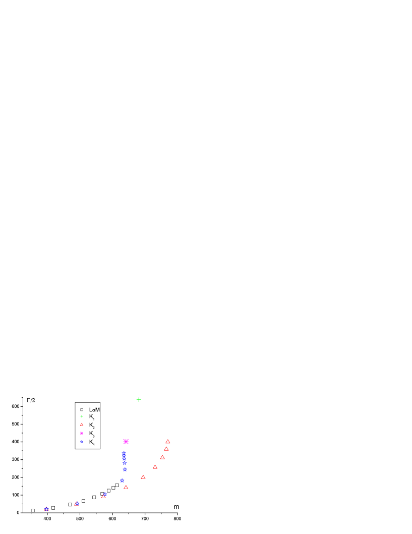
Figure 1: The $\sigma$ pole position from different $K$ matrix unitarizations comparing with the rigorous solution. The open square denotes the exact position of the $O(N)$ model, others are explained in the text.

Poles appeared in $\pi\pi$ scattering are determined by solving the equation $G^{\rm II}=0$, where $G^{\rm II}$ is the analytic continuation of $G$ on the second sheet. From above we realize that the true sigma pole position is a function of the bare sigma mass parameter, for fixed cutoff $\Lambda$. The sigma pole trajectory is plotted in Fig. 1. Throughout this paper we take $v/\sqrt{N}=f_{\pi}=93$MeV and $\Lambda=1.5$GeV. The bare mass of sigma in Fig. 1 ranges from 400MeV to 1200MeV, and each value differs by 100MeV.

In the following we will discuss variations of the above O(N) lagrangian and calculate the scattering amplitude using different unitarization approximations. By comparing with the above rigorous results, we can gain some knowledge on the quality of various approximation methods. It is worth noticing that, for the toy linear O(N) model, it is demonstrated that the [n,n] Padé amplitudes gives the exact sigma pole location, as comparing with the exact solution [16]. The K matrix approach does not reproduce the exact sigma pole location, but it is still a good approximation [16]. In the following we will show that the nice property of these approximation methods will not be maintained if the pion fields are expressed in the non-linear representation.

The next thing we will do is to make polar decomposition of the O(N) field, $i.e.$,

$$\Phi\equiv\varphi\vec{\phi},\,\,\,\phi=(\phi_{1},\phi_{2},......\phi_{N})$$ (14)

with constraint

$$\phi_{1}^{2}+\phi_{2}^{2}+\phi_{3}^{2}+.......+\phi_{N}^{2}=1\ .$$ (15)

In the symmetry breaking phase we define the shifted field,

$$\varphi=\sigma+v$$ (16)

and normalize the field $\vec{\phi}$ as

$$\vec{\pi}=v\vec{\phi}\ .$$ (17)

With above preparations we can obtain the polar decomposition lagrangian,

$$\mathcal{L}_{polar}=\mathcal{L}^{\sigma}+\frac{1}{2}(1+\frac{\sigma}{v})^{2}(\partial_{\mu}\vec{\pi}\cdot\partial^{\mu}\vec{\pi}+\partial_{\mu}\sqrt{v^{2}-\vec{\pi}\cdot\vec{\pi}}\partial^{\mu}\sqrt{v^{2}-\vec{\pi}\cdot\vec{\pi}})$$ (18)

with

$$\mathcal{L}^{\sigma}=\frac{1}{2}\partial_{\mu}\sigma\partial^{\mu}\sigma-\frac{1}{2}m^{2}(\sigma+v)^{2}-\frac{\lambda}{8N}(\sigma+v)^{4}\ .$$ (19)

In the above formula we have used the constraint condition, Eq. (15), so $\vec{\pi}=(\pi_{1},\pi_{2},.....\pi_{N-1})$. Now the symmetry breaking lagrangian, Eq. (2) reads,

$$\mathcal{L}_{SB}=c(\sigma+v)\sqrt{1-\frac{\vec{\pi}\cdot\vec{\pi}}{v^{2}}}\ .$$ (20)

Then we expand the square root to get the interacting vertices which are needed for evaluating $O(p^{4})$ $\pi\pi\to\pi\pi$ processes.

$$\mathcal{L}_{p}=\mathcal{L}^{\sigma}+\frac{1}{2}(1+\frac{\sigma}{v})^{2}(\partial_{\mu}\vec{\pi}\cdot\partial^{\mu}\vec{\pi}+\frac{1}{v^{2}-\vec{\pi}\cdot\vec{\pi}}(\vec{\pi}\cdot\partial_{\mu}\vec{\pi})^{2})+c(\sigma+v)\sqrt{1-\frac{\vec{\pi}\cdot\vec{\pi}}{v^{2}}}$$

$$=\mathcal{L}^{\sigma}+\frac{1}{2}\partial_{\mu}\vec{\pi}\cdot\partial^{\mu}\vec{\pi}+\frac{\sigma}{v}\partial_{\mu}\vec{\pi}\cdot\partial^{\mu}\vec{\pi}+\frac{\sigma^{2}}{2v^{2}}\partial_{\mu}\vec{\pi}\cdot\partial^{\mu}\vec{\pi}+\frac{1}{2v^{2}}(\vec{\pi}\cdot\partial_{\mu}\vec{\pi})^{2}\$$

$$+\frac{1}{2v^{4}}(\vec{\pi}\cdot\partial_{\mu}\vec{\pi})^{2}\vec{\pi}\cdot\vec{\pi}-\frac{m_{\pi}^{2}}{2}\vec{\pi}\cdot\vec{\pi}-\frac{m_{\pi}^{2}}{2v}\sigma\vec{\pi}\cdot\vec{\pi}-\frac{m_{\pi}^{2}}{8v^{2}}(\vec{\pi}\cdot\vec{\pi})^{2}-\frac{m_{\pi}^{2}}{16v^{4}}(\vec{\pi}\cdot\vec{\pi})^{3}$$

$$+\cdots\ .$$ (21)

Notice that in the above lagrangian the $\sigma^{2}\pi^{2}$ term does not contribute to $\pi\pi$ scattering amplitude at 1-loop level since its contribution is 1/N suppressed. There are other variants of the above effective lagrangian. For example we may simply neglect the $\sigma$ field in Eq. (18) and get the O(N) non-linear sigma model

$$\mathcal{L}_{O(N)\,non-linear}=\frac{1}{2}(\partial_{\mu}\vec{\pi}\cdot\partial^{\mu}\vec{\pi}+\partial_{\mu}\sqrt{v^{2}-\vec{\pi}\cdot\vec{\pi}}\partial^{\mu}\sqrt{v^{2}-\vec{\pi}\cdot\vec{\pi}})\ .$$ (22)

Expanding the pion fields from the above lagrangian one gets (also obtainable from Eq. (S0.Ex1) by simply neglecting the sigma field):

$$\mathcal{L}_{NL}=\frac{1}{2}\partial_{\mu}\vec{\pi}\cdot\partial^{\mu}\vec{\pi}-\frac{m_{\pi}^{2}}{2}\vec{\pi}\cdot\vec{\pi}+\frac{1}{2v^{2}}(\vec{\pi}\cdot\partial_{\mu}\vec{\pi})^{2}-\frac{m_{\pi}^{2}}{8v^{2}}(\vec{\pi}\cdot\vec{\pi})^{2}$$

$$+\frac{1}{2v^{4}}(\vec{\pi}\cdot\partial_{\mu}\vec{\pi})^{2}\vec{\pi}\cdot\vec{\pi}-\frac{m_{\pi}^{2}}{16v^{4}}(\vec{\pi}\cdot\vec{\pi})^{3}+\cdots\ .$$ (23)

Also one can integrate out the $\sigma$ field at tree level from Eq. (18) to get a modified O(N) non-linear sigma model:

$$\mathcal{L}_{\overline{NL}}=\mathcal{L}_{NL}+\frac{1}{2m_{\sigma}^{2}v^{2}}[(\partial_{\mu}\vec{\pi}\cdot\partial^{\mu}\vec{\pi})^{2}-m_{\pi}^{2}\vec{\pi}\cdot\vec{\pi}\partial_{\mu}\vec{\pi}\cdot\partial^{\mu}\vec{\pi}+\frac{m_{\pi}^{4}}{4}(\vec{\pi}\cdot\vec{\pi})^{2}].$$ (24)

This lagrangian resembles the $O(p^{4})$ chiral perturbation theory lagrangian.

Starting from Eq. (S0.Ex1) we can calculate the $\pi_{a}\pi_{b}\rightarrow\pi_{c}\pi_{d}$ scattering amplitude up to $O(p^{4})$ in large N limit:

1. The contribution from tree level 4$\pi$ contact term, or current algebra term, denoted as $T_{2}$ ($\sim$$O(p^{2}))$,

   $$T_{2}=\delta_{ab}\delta_{cd}A_{2}(s)+\delta_{ac}\delta_{bd}A_{2}(t)+\delta_{ad}\delta_{bc}A_{2}(u)$$ (25)

   where

   $$A_{2}(s)=\frac{1}{v^{2}}(s-m_{\pi}^{2})\ .$$ (26)

2. The contribution from tree level $O(p^{4})$ term contained in Eq. (24), denoted as $T_{4}$, is

   $$T_{4}=\delta_{ab}\delta_{cd}A_{4}(s)+\delta_{ac}\delta_{bd}A_{4}(t)+\delta_{ad}\delta_{bc}A_{4}(u)$$ (27)

   where

   $$A_{4}(s)=\frac{(s-m_{\pi}^{2})^{2}}{m_{\sigma}^{2}v^{2}}\ .$$ (28)

3. The contribution from tree level $\sigma$ exchange in Eq. (S0.Ex1) ($\sim O(p^{4})$),

   $$T_{\sigma}=\delta_{ab}\delta_{cd}A_{\sigma}(s)+\delta_{ac}\delta_{bd}A_{\sigma}(t)+\delta_{ad}\delta_{bc}A_{\sigma}(u)$$ (29)

   where

   $$A_{\sigma}(s)=\frac{-1}{v^{2}}\frac{(s-m_{\pi}^{2})^{2}}{s-m_{\sigma}^{2}}\ ,$$ (30)

   which is $O(p^{4})$ at low energies.

4. The contribution from 1-loop diagrams (in large N limit and including only $O(p^{4})$ terms):

   $$T_{loop}=\delta_{ab}\delta_{cd}A_{loop}(s)+\delta_{ac}\delta_{bd}A_{loop}(t)+\delta_{ad}\delta_{bc}A_{loop}(u)$$ (31)

   where

   $$A_{loop}=\frac{N}{v^{4}}[(s-m_{\pi}^{2})^{2}B_{0}(s;m_{\pi}^{2})-i\frac{3m_{\pi}^{2}-2s}{2}\int\frac{d^{D}k}{(2\pi)^{D}}\frac{1}{k^{2}-m_{\pi}^{2}}]\ .$$

The quadratic divergent integral from bubble diagram in above is treated in the standard way in dimensional regularization scheme,

$$\int\frac{d^{D}k}{(2\pi)^{D}}\frac{1}{k^{2}-m^{2}}=im^{2}\Delta-\frac{i}{16\pi^{2}}\widetilde{A}(m^{2})\ ,$$ (33)

where

$$\widetilde{A}(m^{2})=-m^{2}\ .$$ (34)

As before we introduce the cutoff in the same way as in calculating the solvable linear $O(N)$ model, i.e.,

$$\Gamma(\epsilon)+\ln{4\pi}+\ln{\frac{\nu^{2}}{m^{2}}}\Rightarrow\ln{\frac{\Lambda^{2}}{m^{2}}}\ .$$

One can check that the above treatment to ignore the square cutoff leads to the same result in the chiral limit to 1-loop amplitude comparing with the one obtained from the original $O(N)$ model.

Now consider the I=0 channel,

$$T^{I=0}(s,t,u)=(N-1)A(s)+A(t)+A(u)\ .$$ (35)

In the large N limit, only the $s$ channel amplitude $A(s)$ term survives. The J=0 partial wave is simply

$$T^{00}=\frac{1}{32\pi}NA(s)\ .$$ (36)

With the above preparation we will in the following construct various unitarized amplitudes based on tree and one loop calculations using different lagrangians. The unitary amplitudes being constructed are: $K_{1}$ (using tree level amplitude in pure $O(N)$ non-linear $\sigma$ model), $K_{2}$ ($K_{1}$ plus $\sigma$ exchange), $K_{3}$ (1-loop calculation in the pure $O(N)$ non-linear $\sigma$ model), $K_{4}$ (1-loop with $\sigma$ exchange included using polar decomposed lagrangian); as well as $P_{1}$ ([1,1] Padé for the pure $O(N)$ non-linear $\sigma$ model), $P_{2}$ ([1,1] Padé with the $\sigma$ being integrated out, i.e., of Eq. (24)), $P_{3}$ ([1,1] Padé with explicit $\sigma$ exchange, i.e., of Eq. (24)). For simplifying the expressions we in the following use $v$ (=93MeV) to replace $v/\sqrt{N}$. In the following we will always work in the IJ=00 channel and hence for simplicity we drop out the superscripts 00 in the partial wave amplitude.

$K_{1}$ amplitude:

This approximation corresponds to the simplest $K$ matrix amplitude in the pure O(N) non-linear sigma model. Also it is the simplest $K$ matrix amplitude one obtains from Eq. (S0.Ex1). One has

$$S=\frac{1+i\rho K}{1-i\rho K}\ .$$ (37)

Here $K_{1}=T_{2}$ and hence

$$S=\frac{1+i\rho T_{2}}{1-i\rho T_{2}}\ ,$$ (38)

where $\rho=\sqrt{1-4m_{\pi}^{2}/s}$ and

$$T_{2}=\frac{1}{32\pi v^{2}}(s-m_{\pi}^{2})\ .$$ (39)

The dynamically generated second sheet poles correspond to the zeros of the $S$ matrix, we show the pole position in Fig. 1 labeled as $K_{1}$. Notice that there is no free parameter here. We see from Fig. 1 that $K_{1}$ is not a good approximation numerically to the real solution (i.e., the solution of the linear sigma model). There is another serious disadvantage in this approximation, which can be clearly seen in the chiral limit. That is the pole location, $\sqrt{s_{p}}$, is proportional to $v$ and hence is proportional to the square root of the number of colors, $N_{c}$:

$$\sqrt{s_{p}}\propto\sqrt{i32\pi f_{\pi}^{2}}\propto\sqrt{N_{c}}\ .$$ (40)

So when $N_{c}\to\infty$ this pole disappears! On the other side the sigma pole in the linear sigma model behaves as $m_{\sigma}\sim O(N_{c}^{0})$ in $N_{c}$ power counting.

$K_{2}$ amplitude:

$K_{2}=T_{2}+T_{\sigma}$. This approximation corresponds to calculating the scattering amplitude at tree level in the polar decomposition lagrangian Eq. (S0.Ex1), and it is also equivalent to the lowest order $K$ matrix amplitude evaluated in the linear sigma model. We have,

$$S=\frac{1+i\rho(T_{2}+T_{\sigma})}{1-i\rho(T_{2}+T_{\sigma})}\ ,$$ (41)

with

$$T_{\sigma}=\frac{-1}{32\pi v^{2}}\frac{(s-m_{\pi}^{2})^{2}}{s-m_{\sigma}^{2}}\ ,$$ (42)

and

$$K_{2}=T_{2}+T_{\sigma}=\frac{s-m_{\pi}^{2}}{32\pi v^{2}}\frac{m_{\pi}^{2}-m_{\sigma}^{2}}{s-m_{\sigma}^{2}}\ .$$

The second sheet poles correspond to the solution of the following equation,

$$s-m_{\sigma}^{2}+i\sqrt{\frac{s-4m_{\pi}^{2}}{s}}\frac{1}{32\pi v^{2}}(m_{\pi}^{2}-m_{\sigma}^{2})(s-m_{\pi}^{2})=0\ .$$ (43)

The pole trajectory is plotted in Fig. 1 labeled as $K_{2}$. Apparently $K_{2}$ works much better than $K_{1}$. Especially the pole position is now $\sqrt{s_{p}}\sim O(N_{c}^{0})$. But numerically it is still a rather poor approximation as can be seen from Fig. 1.

By analyzing the $K_{2}$ approximant one can learn an important lesson. It is easy to find solution of Eq. (43) in the chiral limit:

$$s_{pole}=\frac{m_{\sigma}^{2}}{1-\frac{im_{\sigma}^{2}}{32\pi v^{2}}}\ .$$ (44)

In the above equation if one formally sends $m_{\sigma}\to\infty$ one recovers the solution Eq. (40) in the chiral limit, $i.e.$, $s_{pole}=i32\pi v^{2}\to\infty$ when $N_{c}\to\infty$. Nevertheless if one firstly take the large $N_{c}$ limit in Eq. (44) one gets simply $s_{pole}=m_{\sigma}^{2}$. Apparently the latter one is the correct relation we are looking for. Therefore we conclude that one must take the large $N_{c}$ limit before integrating out the sigma degree of freedom in order to get the correct large $N_{c}$ spectrum.

$K_{3}$ amplitude:

$K_{3}=T_{2}+{\rm Re}[T_{loop}]$. This approximation corresponds to a 1–loop calculation in the pure O(N) non-linear sigma model. Notice that here we adopt the cutoff effective lagrangian approach, therefore no renormalization procedure and hence no counter terms are needed.

$$S=\frac{1+i\rho(T_{2}+{\rm Re}[T_{loop}])}{1-i\rho(T_{2}+{\rm Re}[T_{loop}])}$$ (45)

with

$$T_{loop}=\frac{1}{64\pi v^{4}}\frac{1}{16\pi^{2}}\{(s-m_{\pi}^{2})^{2}[2+\ln{\frac{\Lambda^{2}}{m_{\pi}^{2}}}+\rho(s)(\ln\frac{1-\rho(s)}{1+\rho(s)}+i\pi)]$$

$$+(3m_{\pi}^{2}-2s)m_{\pi}^{2}(1+\ln{\frac{\Lambda^{2}}{m_{\pi}^{2}}})\}\ .$$ (46)

Notice that in this approximation the sigma pole is dynamically generated and its location is also fixed. The pole position is shown in Fig. 1 labeled as $K_{3}$. Notice that here, like the $K_{1}$ case, one also has $\sqrt{s_{p}}\sim O(N_{c}^{1/2})$.

$K_{4}$ amplitude:

$K_{4}=T_{2}+T_{\sigma}+Re(T_{loop})$. This approximation corresponds to considering all contributions up to $O(p^{4})$ term in the polar decomposed O(N) model. We have

$$S=\frac{1+i\rho[T_{2}+T_{\sigma}+Re(T_{loop})]}{1-i\rho[T_{2}+T_{\sigma}+Re(T_{loop})]}\ .$$ (47)

The pole trajectory is plotted in Fig. 1, labeled as $K_{4}$. Comparing with $K_{2}$, the quality of the result is not actually improved. What is even worse here is that the $K_{4}$ amplitude contains a spurious pole on the second sheet, not far from the sigma pole position.

We conclude in general that the $K$ matrix unitarization approach to the amplitude obtained from a lagrangian with non-linearly realized chiral symmetry does not work very well. Still, there exist other distant spurious poles (can be on both sheets) in these $K$ matrix amplitudes, which are not shown in Fig. 1. On the contrary, the $K$ matrix approach works fairly well on the linear O(N) model.

In the following we turn to discuss the Padé approximations which are very frequently used in phenomenological discussions. Notice that Padé amplitudes also preserve one bad heritage of the original exact amplitude – the tachyon pole. But as stated before the appearance of the tachyon pole does not matter in practice in the phenomenological discussions.

$P_{1}$ amplitude:

This approximation corresponds to the [1,1] Padé approximation in the cutoff pure non-linear O(N) model,

$$T=\frac{T_{2}^{2}}{T_{2}-T_{loop}}\ .$$ (48)

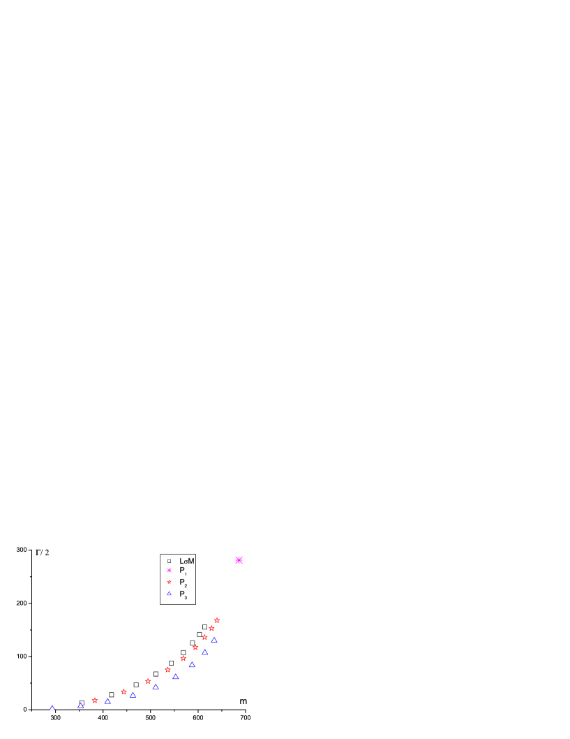
Figure 2: The $\sigma$ pole position from different Padé approximations comparing with the rigorous solution. The open square denotes the exact position of the $O(N)$ model, others are explained in the text.

The pole position is shown in Fig. 2 labeled as $P_{1}$. Certainly it is better than $K_{1}$ but similar in quality with $K_{3}$. The same problem remains, however, that is $\sqrt{s_{p}}\propto v\propto O(N_{c}^{1/2})$.

$P_{2}$ amplitude:

This approximant corresponds to a 1-loop calculation using $\cal{L}_{\overline{NL}}$ of Eq. (24):

$$T=\frac{T_{2}^{2}}{T_{2}-T_{4}-T_{loop}}$$ (49)

where

$$T_{4}=\frac{(s-m_{\pi}^{2})^{2}}{32\pi v^{2}m_{\sigma}^{2}}\ .$$ (50)

Second sheet poles are determined by solving the following equation,

$$s-m_{\pi}^{2}-\frac{(s-m_{\pi}^{2})^{2}}{m_{\sigma}^{2}}-\frac{1}{32\pi^{2}v^{2}}\{(s-m_{\pi}^{2})^{2}[2+\ln{\frac{\Lambda^{2}}{m_{\pi}^{2}}}+\rho(\ln{\frac{1-\rho}{1+\rho}}-i\pi)]$$

$$+(3m_{\pi}^{2}-2s)m_{\pi}^{2}(1+\ln{\frac{\Lambda^{2}}{m_{\pi}^{2}}})\}=0$$ (51)

The pole trajectory is shown in Fig. 2 labeled as $P_{2}$. This approximation is the best among all. It is not difficult to examine using Eq. ($P_{2}$ amplitude:) that if one takes the large $N_{c}$ limit one finds $\sqrt{s_{p}}\simeq m_{\sigma}$. On the other sides, if one sends $m_{\sigma}\to\infty$ before taking the large $N_{c}$ limit one gets $\sqrt{s_{p}}\propto v\sim O(N_{c}^{1/2})$. Once again we find that the $m_{\sigma}\to\infty$ limit and the large $N_{c}$ limit do not commute.

$P_{3}$ amplitude:

This approximation corresponds to the [1,1] Padé approximation up to $O(p^{4})$ term in the polar decomposition lagrangian Eq. (S0.Ex1). We have,

$$T=\frac{T_{2}^{2}}{T_{2}-T_{\sigma}-T_{loop}}\ .$$ (52)

The pole trajectory is plotted in Fig. 2 labeled as $P_{3}$. Notice that adding a sigma pole explicitly in the lagrangian does not improve the quality of output. What is even worse is that it also predicts a spurious pole not very far from the sigma pole. Our analysis seems to suggest that a polar decomposed sigma model lagrangian works even worse than the situation when the sigma field is completely integrated out. It is however not clear whether this observation remain valid in the realistic case.

The pole appeared in the unitarized amplitude is dynamical in the case of $O(N)$ non-linear $\sigma$ model, and also dynamical in the case of Eq. (24). In the former case the pole moves to infinity as $N_{c}\to\infty$ whereas in the latter case the pole falls down to the real axis when $N_{c}\to\infty$. For the latter we know that the dynamical pole is nothing but just represents the original $\sigma$ pole being integrated out from Eq. (S0.Ex1) or Eq. (1), as is revealed by the simple exercise on $P_{2}$ amplitude, hence ‘elementary’ in its origin. The drastically different $N_{c}$ dependence of the pole trajectories, in our understanding, merely reflects the different order when taking the large $N_{c}$ and $m_{\sigma}\to\infty$ limits.

In a more realistic calculation however, the inverse problem becomes problematic since the Padé approximants for chiral perturbation theory bring, together with the sigma pole, also spurious poles and some of which violate analyticity [14]. Nevertheless the toy model we discussed here well resembles many aspects of the real situation. For example we pointed out that in the simplest $K_{1}$ approximant, the dynamical pole being generated has the deferent $N_{c}$ behavior comparing with the $\sigma$ meson in the linear O(N) model. The situation is very similar in realistic case. In Ref. [18], based upon a [0,1] Padé or $K_{1}$ approximant the authors suggest that the current algebra term dominates at low energy, since the pole position of the sigma meson obtained as such is,

$$\sqrt{s_{\sigma}}\simeq\sqrt{16i\pi f_{\pi}^{2}}\simeq 463-463i\ ,$$ (53)

and is found to be not far from the pole position obtained from a more careful numerical analysis. According to the analysis made in this paper, even though the current algebra term dominates low energy physics, the $N_{c}$ dependence of the pole trajectory in Eq. (53) does not in any sense prove that the $\sigma$ pole is dynamical. The current algebra term in Eq. (S0.Ex1) gives exactly the same $N_{c}$ dependence as in Eq. (53) meanwhile it comes from the $linear$ sigma model with explicit $\sigma$ degree of of freedom! If Eq. (53) were correct for arbitrarily large $N_{c}$, the pole will move to infinity when $N_{c}\to\infty$, hence contradicting the $N_{c}$ counting rule for a conventional meson state. If this were true the sigma meson had to be a dynamical pole. Going beyond the leading current algebra amplitude, contrary to what is claimed in Ref. [19], in the [1,1] Padé approximant in reality, the $\sigma$ pole actually finally falls on the real axis. That is the pole position as given in Eq. (53) receive important corrections when $N_{c}$ is large:

$$s_{\sigma}=\frac{16i\pi f_{\pi}^{2}}{1+16i\pi f_{\pi}^{2}\triangle}\ ,$$

$$\triangle=\frac{2}{3f_{\pi}^{2}}(22L_{1}+14L_{2}+11L_{3})\propto O(N_{c}^{0})\ ,$$ (54)

valid in the large $N_{c}$ and chiral limit. It is worth noticing that it was not clear what is the approximation made to obtain Eq. ($P_{3}$ amplitude:). Using the PKU parametrization form [4, 5, 6] one explicitly demonstrates that the Eq. ($P_{3}$ amplitude:) is obtained under two further assumptions: 1) assuming one pole (the $\sigma$ pole) dominates in the $s$ channel at low energies; 2) neglecting all the crossed channel resonance exchanges [20]. It is understood that the assumption 1 actually fixes the $N_{c}$ behavior of the $\sigma$ pole, i.e., $m_{\sigma}\sim O(1)$, $\Gamma_{\sigma}\sim O(1/N_{c})$ [21, 20]. The assumption 2 does no harm in distorting the large $N_{c}$ behavior. However, these assumptions are only approximately correct when $N_{c}=3$ and fail at large $N_{c}$, as demonstrated in Ref. [22]. Actually it is likely that at large $N_{c}$, crossed channel resonance exchange dominates low energy physics. Hence Eq. ($P_{3}$ amplitude:) can neither be used to discuss the large $N_{c}$ behavior of the $\sigma$ pole trajectory. In Ref. [19], it is observed that, unlike the $\rho$ meson which almost falls straightforwardly down to the real axis when $N_{c}$ increases, the $\sigma$ meson is very unwilling to fall down. Based on this observation the authors of Ref. [19] concluded that the $\sigma$ pole they found from their unitarized amplitude a dynamically generated one. Even if Eq. ($P_{3}$ amplitude:) is invalid to be useful when discussing the large $N_{c}$ behavior of the $\sigma$, the discussions given in this paper make it clear that the bent structure of the $\sigma$ pole trajectory should not be used to argue that the $\sigma$ is dynamical.  We plot in Fig. 3 the $N_{c}$ dependence of the $\sigma$ pole in linear $O(N)$ model (as well as the $P_{2}$ approximant). Fig. 3 clearly shows that, even the ‘elementary’ $\sigma$ does not fall down to the real axis straightforwardly. Though not a rigorous proof, in our opinion the similar bent structure of the $\sigma$ pole trajectory both in Fig. 3 and in the unitarized chiral perturbation theory amplitude suggest one simple thing: the observed $f_{0}(600)$ state is the $\sigma$ meson being responsible for the spontaneous breaking of chiral symmetry. In 1+1 dimensions, using an exact solution for the large-N limit, Ref. [23] showed dynamical generation of the sigma meson starting with the nonlinear sigma model. In 4 dimensions the situation remains to be understood. In any case in the linear $\sigma$ model the $\sigma$ meson is the chiral partner of the pseudo-goldstone bosons and the two mix each other under chiral rotations. It suggests that the $\sigma$ meson shares one dynamical property of the pion, i.e., being a collective mode. Hence the appropriate way to describe it is not to consider it as dynamically generated from pion fields, rather it should be discussed at the equal level as pions in the effective lagrangian approach. Also the $\sigma$ meson should not be properly described by any simple quark models since a pion can not be.

This work is supported in part by National Natural Science Foundation of China under contract number 10575002 and 10421503.

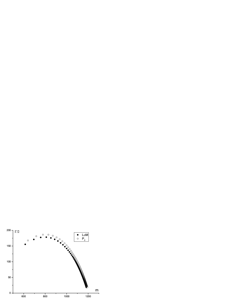
Figure 3: $N_{c}$ dependence of the $\sigma$ pole position. Full circle: linear $O(N)$ sigma model; open circle: $P_{2}$ approximation. In drawing the plot $N_{c}$ starts from 3 and each pole is differed by increasing $N_{c}$ by 1. The bare mass $m_{\sigma}$ is taken as 1.2GeV.

References

- [1] Z. G. Xiao and H. Q. Zheng, Nucl. Phys. A695 (2001) 273.
- [2] I. Caprini, G. Colangelo and H. Leutwyler, Phys. Rev. Lett. 96 (2006) 132001.
- [3] S. Descotes-Genon, B. Moussallam, hep-ph/0607133.
- [4] H. Q. Zheng , Nucl. Phys. A733 (2004) 235.
- [5] Z. Y. Zhou , JHEP0502 (2005) 43.
- [6] Z. Y. Zhou and H. Q. Zheng, Nucl. Phys. A755 (2006) 212.
- [7] A. Höll, P. Maris, C.D. Roberts and S.V. Wright, Nucl. Phys. Proc. Suppl. 161:87-94,2006 (nucl-th/0512048).
- [8] N. A. Tornqvist, Z. Phys. C68(1995)647; N. N. Achasov and G. N. Shestakov, Phys. Rev. D49(1994)5779; R. Kaminski, L. Leśniak and J.-P. Maillet, Phys. Rev. D50(1994)3154; M. Ishida, S. Ishida and T. Ishida, Prog. Theor. Phys. 99(1998)1031; D. Black , Phys. Rev. D64 (2001) 014031.
- [9] M. D. Scadron, F. Kleefeld, G. Rupp, E. van Beveren, Nucl. Phys. A724(2003)391.
- [10] A. Gomez Nicola, J. R. Pelaez, Phys. Rev. D65(2002)054009; J. A. Oller, E. Oset, J. R. Pelaez, Phys. Rev. D59(1999)074001, Erratum-ibid. D60(1999)099906.
- [11] J. R. Pelaez, Mod. Phys. Lett. A19(2004)2879.
- [12] J. L. Basdevant and B. W. Lee, Phys. Rev. D2(1970)1680.
- [13] J. L. Basdevant and J. Zinn-Justin, Phys. Rev. D3(1971)1865.
- [14] G. Y. Qin et al., Phys. Lett. B542(2002)89.
- [15] S. Coleman, R. Jackiw and H. D. Politzer, Phys. Rev. D10(1974)2491.
- [16] S. Willenbroch, Phys. Rev. D43(1990)1710.
- [17] Y. B. Dai, Y. L. Wu, Eur. Phys. J.C39(2005)S1.
- [18] G. Colangelo, J. Gasser and H. Leutwyler, Nucl. Phys. B603(2001)125; H. Leutwyler, hep-ph/0608218, contributions to MESON2006.
- [19] J. R. Pelaez, Phys. Rev. Lett. 92(2004)102001.
- [20] Z. X. Sun, L. Y. Xiao, Z. G. Xiao and H. Q. Zheng, talk given at International Conference on Nonperturbative Quantum Field Theory: Lattice and Beyond, Guangzhou, Canton, China, 18-20 Dec 2004, Mod. Phys. Lett. A22(2007)711.
- [21] Z. G. Xiao and H. Q. Zheng, Mod. Phys. Lett. A22(2007)55.
- [22] Z. H. Guo, J. J. Sanz Cillero, H. Q. Zheng, hep-ph/0701232, to appear in JHEP.
- [23] W. Bardeen, B. W. Lee, and R. E. Shrock, Phys. Rev. D14(1976) 985.