Microscopic derivation of the pion coupling to heavy–light mesons

Abstract

The Goldberger–Treiman relation for heavy–light systems is derived in the context of a quark model. As a paradigmatic example, the case of ${\bar{D}}\to{\bar{D}}^{\prime}\pi$ is studied in detail. The fundamental role played by the pion two-component wave function, in the context of the Salpeter equation, is emphasized.

I Introduction

Quark models endowed with effective quark current-current microscopic interactions, consistent with the requirements of chiral symmetry, have provided, through the years, an invaluably useful tool towards the construction of an effective low–energy theory for the strong interactions Orsay ; Orsay2 ; Lisbon ; linear ; ASES . Besides regularizing the ultraviolet divergences of the theory, these effective theories bring in the necessary interaction scale needed to make contact with the hadronic phenomenology. An important feature of this class of models is the essential convergence of results and conclusions across a variety of possible forms for the confining kernel. They fulfill the well–known low energy theorems of Gell–Mann, Oakes, and Renner Orsay2 , Goldberger and Treiman Lisbon , the Weinberg theorem EmilCota , and so on. Using this formalism it is also possible to give, for this class of models, an analytic proof of the low–energy theorems in the light–quark sector BicudAp . It turns out that the chiral angle — the solution to the mass-gap equation— remains the only nontrivial characteristic of such a class of models and it defines the latter completely.

In the present paper, we derive the generalized Goldberger–Treiman (GT) relation for the heavy–light systems. The heavy–light mesons have received a lot of attention in the past few years due to the discovery of new narrow states in the $c{\bar{s}}$ family ds . Nowak et al. Nowak and Bardeen and Hill BH have postulated that the spectrum of such states should reflect the pattern of dynamical chiral symmetry breaking. Namely in the heavy–quark limit, the mass spectrum is expected to be determined by the light quark and, were chiral symmetry to be exact, the heavy–light states of opposite parity would have become degenerate. It then follows that physical splitting between parity doublers could be related to the scale of spontaneous breaking of chiral symmetry, that is the quark condensate or, phenomenologically, to the constituent quark mass. As more states in the open charm sector have been reported, alternative pictures have been examined, making this sector a good testing ground for phenomenological models others . Recently, for example, a canonical, quark model description has been investigated and it was argued that the new $D_{s}$ states can in fact be described as quark model states eric . Notwithstanding the phenomenological successes of the naive quark model, it suffers from the serious shortcoming of being unable to account for the physics of chiral symmetry breaking. It therefore fails, among other issues basically related to pion physics, to constrain the treatment of strong decays by the underlying bound state dynamics. This failure results, for example, in predictions for couplings to the ground–state pseudoscalars which do not satisfy PCAC or the Goldberger–Treiman relations Close:2005se . Roughly speaking, quark models consistent with chiral symmetry can be thought of being evolutions of the naive quark model supplemented by the constraint of the mass-gap equation, and therefore they should provide the correct framework to study such strong decays. Here we shall show that such type of models leads indeed to the GT relation for the pion coupling between the opposite–parity states. This is a non-trivial result, which can only follow from the simultaneous use of a chiral invariant interaction together with a consistent treatment of the pion and heavy–light meson dynamics.

The paper is organized as follows. In the following section we recapitulate the chiral quark models and discuss the application to the ground–state pseudoscalar and heavy-quark sectors. In Section III, we present the proof of the Goldberger–Treiman relation for the heavy–light mesons. Summary and a brief discussion are given in Section IV. Throughout the paper we concentrate on the $J^{P}=0^{\mp}$ heavy–light states, but the results can easily be generalized to higher spins.

II Chiral quark models

In this chapter, we give a short introduction to the chiral quark model. The model is described by the Hamiltonian

$$H = \int d^{3}x\psi^{{\dagger}}({{\bf x}})\left(-i{\bm{\alpha}}\cdot{\bm{\bigtriangledown}}+m\beta\right)\psi({{\bf x}})$$ (1)

$$+ \frac{1}{2}\int d^{3}xd^{3}y\;J^{a}_{\mu}({{\bf x}})K^{ab}_{\mu\nu}({{\bf x}}-{{\bf y}})J^{b}_{\nu}({{\bf y}}),$$

with the quark current–current ($J_{\mu}^{a}({{\bf x}})=\bar{\psi}({{\bf x}})\gamma_{\mu}\frac{\lambda^{a}}{2}\psi({{\bf x}})$) interaction parameterized by the instantaneous confining kernel $K^{ab}_{\mu\nu}({{\bf x}}-{{\bf y}})$. An important feature of the models of the class (1) is the remarkable robustness of their predictions with respect to variations of the quark kernel. Although quantitative results may vary for different kernels, the qualitative picture described remains essentially the same. This is specially true for those relations enforced by the mechanism of chiral symmetry breaking that should be independent of the spatial details of the confining kernel provided it brings a natural confinement scale (hereafter called $K_{0}$). The only requirement is that it should be chirally symmetric. We illustrate this nice feature by deriving the Goldberger–Treiman relation connecting the pion coupling to heavy–light mesons to the mass splitting between chiral doublets, for the simplest Lorentz structure of the inter-quark interaction in the Hamiltonian (1) compatible with the requirements of chiral symmetry and confinement $K_{\mu\nu}^{ab}({\bf x}-{\bf y})=\delta^{ab}g_{\mu 0}g_{\nu 0}V(|{\bf x}-{\bf y}|)$ Orsay ; Lisbon ; ASES ; Szczepaniak:1996tk , for an arbitrary confining kernel $V(r)$. We also note that analogous Hamiltonian with linearly rising potential considered in one time and one spatial dimension reproduces the ’t Hooft model for 2D QCD tHooft in the Coulomb (axial) gauge (see, for example, the original paper BG or the review paper 2d and references therein).

A standard way of proceeding with the investigation of the model (1) is to consider the self-interaction of quarks separately, thus introducing the notion of the dressed quarks:

$$\psi({\bf x})=\sum_{\zeta=\uparrow,\downarrow}\int\frac{d^{3}p}{(2\pi)^{3}}e^{i{\bf p}{\bf x}}[b_{\zeta}({\bf p})u_{\zeta}({\bf p})+d_{\zeta}^{+}(-{\bf p})v_{\zeta}(-{\bf p})],$$ (2)

where the quark amplitudes

$$\begin{array}[]{rcl}u({\bf p})&=&\displaystyle\frac{1}{\sqrt{2}}\left[\sqrt{1+s_{p}}+({\bm{\alpha}}\cdot\hat{{\bf p}})\sqrt{1-s_{p}}\right]u_{0}({\bf p}),\\[14.22636pt] v(-{\bf p})&=&\displaystyle\frac{1}{\sqrt{2}}\left[\sqrt{1+s_{p}}-(\bm{\alpha}\cdot\hat{{\bf p}})\sqrt{1-s_{p}}\right]v_{0}(-{\bf p})\end{array}$$ (3)

are parameterized with the help of the chiral angle $\varphi_{p}$ Orsay ; Orsay2 ; Lisbon , $s_{p}=\sin\varphi_{p}$, $c_{p}=\cos\varphi_{p}$. It is convenient to define the chiral angle varying in the range $-\pi/2<\varphi_{p}\leq\pi/2$, with the appropriate boundary conditions $\varphi(0)=\frac{\pi}{2}$, $\varphi(p\to\infty)\to 0$ for the physical vacuum. The equation which defines the profile of the chiral angle — the mass-gap equation — follows from the requirement that the quadratic part of the normally ordered Hamiltonian (1) should be diagonal in terms of the dressed quark creation and annihilation operators Lisbon . The mass-gap equation then takes the form:

$$mc_{p}-ps_{p}=\frac{C_{F}}{2}\int\frac{d^{3}k}{(2\pi)^{3}}V({\bf p}-{\bf k})[s_{k}c_{p}-xc_{k}s_{p}],$$ (4)

where $x=(\hat{{\bf p}}\cdot\hat{{\bf k}})$. In Fig. 1, we give a typical profile of the chiral angle.

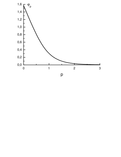
Figure 1: A typical profile of the chiral angle — solution to the mass-gap equation. Momentum $p$ is measured in the units of the potential strength $K_{0}$.

The dressed quark dispersive law can be evaluated then as

$$E_{p}=ms_{p}+pc_{p}+\frac{C_{F}}{2}\int\frac{d^{3}k}{(2\pi)^{3}}V({\bf p}-{\bf k})\left[s_{p}s_{k}+xc_{p}c_{k}\right].$$ (5)

We turn now to bound states of dressed quarks — to the quark–antiquark mesons. Each mesonic state in this model is described with a two–component wave function, and the bound–state equation acquires the form of a system of two coupled equations. The details can be found in the works Orsay2 ; Lisbon , where the Bethe–Salpeter equation formalism was developed or in Ref. nr , where a second Bogoliubov-like transformation is performed over the Hamiltonian (1) in order to define explicitly the compound mesons creation and annihilation operators. For the purpose of the present research, it is sufficient to consider two particular cases of this general mesonic bound–state equation.

II.1 The case of the chiral pion

In the chiral limit, the bound–state equation for the pion at rest is known to be given by the mass-gap equation (4) with $m=0$ Lisbon ; nr . In the random phase approximation (RPA) both components of the pionic wave function coincide and are simply $\sin\varphi_{p}$ Orsay2 ; Lisbon ; nr . Beyond the chiral limit, the pion state is given by $({\bf p}_{\pi}=0)$:

$$|\pi^{i}\rangle=\int\frac{d^{3}k}{(2\pi)^{3}}\left[b^{\dagger}({\bf k})\frac{\tau^{i}}{\sqrt{N_{f}}}\frac{I_{c}}{\sqrt{N_{C}}}\frac{I_{s}}{\sqrt{2}}d^{\dagger}(-{\bf k})X({\bf k})\right.$$

(6)

$$+\left.d(-{\bf k})\frac{\tau^{i}}{\sqrt{N_{f}}}\frac{I_{c}}{\sqrt{N_{C}}}\frac{I_{s}}{\sqrt{2}}b({\bf k})Y({\bf k})\right]|0\rangle,$$

with $|0\rangle$ being the broken BCS vacuum. $N_{f}$ and $N_{C}$ are, respectively, the number of flavors and colors.

The normalized wave functions are given by

$$X({\bf k})=\frac{\sqrt{N_{C}}\sqrt{N_{s}}\sqrt{N_{f}}}{2if_{\pi}}[s_{k}+m_{\pi}\Delta_{k}],$$

(7)

$$Y({\bf k})=\frac{\sqrt{N_{C}}\sqrt{N_{s}}\sqrt{N_{f}}}{2if_{\pi}}[s_{k}-m_{\pi}\Delta_{k}],$$

with $\Delta_{k}$ satisfying

$$2E_{k}\Delta_{k}=s_{k}+C_{F}\int\frac{d^{3}q}{(2\pi)^{3}}V({\bf k}-{\bf q})[s_{k}s_{q}+xc_{k}c_{q}]\Delta_{q}.$$ (8)

II.2 The case of a heavy–light meson

The case of a heavy–light meson, with one quark being infinitely heavy, leads to considerable simplifications of the bound–state equation in view of the fact that the negative energy–spin component of the meson wave function, responsible for the time–backward motion of the quark–antiquark pair, which is non-negligible for the light-light system, goes to zero with the bare mass increase of just one quark of the pair (heavy–light systems), vanishing in the infinite mass limit of that quark. The resulting equation takes the form of a Schrödinger-like equation parity

$$E_{p}\hat{\Psi}({\bf p})+\int\frac{d^{3}k}{(2\pi)^{3}}V({\bf p}-{\bf k})\left[C_{p}C_{k}+\right.\hskip 28.45274pt$$

(9)

$$\hskip 28.45274pt\left.({\bm{\sigma}}\cdot\hat{{\bf p}})({\bm{\sigma}}\cdot\hat{{\bf k}})S_{p}S_{k}\right]\hat{\Psi}({\bf k})=E\hat{\Psi}({\bf p}),$$

with

$$C_{p}=\frac{1}{\sqrt{2}}\left[\sqrt{1+c_{p}}+\sqrt{1-c_{p}}\right],\quad$$

(10)

$$S_{p}=\frac{1}{\sqrt{2}}\left[\sqrt{1+c_{p}}-\sqrt{1-c_{p}}\right].$$

Here the wave function is written as a product of the orbital part and the spin part, $\hat{\Psi}(k)=I/\sqrt{2}\cdot\Psi(k)$ for the $J^{P}=0^{-}$ and $\hat{\Psi}^{\prime}(k)=({\bm{\sigma}}\cdot\hat{\bf k})/\sqrt{2}\cdot\Psi^{\prime}(k)$ for the $J^{P}=0^{+}$ heavy–light meson, respectively. The conventional normalization of the wave function (consistent with the relativistic normalization) is

$$2M=\int\frac{d^{3}k}{(2\pi)^{3}}|\Psi({\bf k})|^{2}=\int\frac{d^{3}k}{(2\pi)^{3}}|\Psi^{\prime}({\bf k})|^{2},$$ (11)

where, in the heavy–quark limit, $M$ approximates the mass of the heavy quark, and the mass of the heavy–light meson is given by $M+E$.

III Goldberger–Treiman relation for heavy–light mesons

In this chapter, we focus on the details of the pion interaction with heavy–light mesons. Consider the hadronic process which involves the chiral pion and the two heavy–light mesons for which, for the sake of transparency, we consider the ${\bar{D}}(J^{P}=0^{+})$ and the ${\bar{D}}^{\prime}(J^{P}=0^{-})$ mesons with the wave functions $\hat{\Psi}(k)$ and $\hat{\Psi}^{\prime}(k)$, respectively.

III.1 The macroscopic derivation of the Goldberger–Treiman relation in QCD

Let us consider the transition ${\bar{D}}\to{\bar{D}}^{\prime}\pi$. Then, using the relation

$$\langle 0|A^{a}_{\mu}(0)|\pi^{b}({\bf q})\rangle=if_{\pi}q_{\mu}\delta^{ab},$$ (12)

we introduce the $nn^{\prime}\pi$ coupling $g_{nn^{\prime}\pi}$ through the relation

$$\langle n^{\prime}|A^{a}_{\mu}|n\rangle=\langle n^{\prime}|A_{\mu}^{a}|n\rangle_{\mbox{nonpion}}-\frac{2Mq_{\mu}f_{\pi}g_{nn^{\prime}\pi}}{q^{2}-m_{\pi}^{2}+i\epsilon}D^{{}^{\prime}{\dagger}}\tau^{a}D,$$ (13)

where the subscript “nonpion” denotes the contribution free of the pion pole. Here $D^{\prime}$, $D$ are unit isospin doublets representing the flavor of the heavy–light $n^{\prime}$ and $n$ state, respectively.

On the other hand, the full matrix element of the axial current, corresponding to the l.h.s. of Eq. (13) can be written as:

$$\langle n^{\prime}|A^{a}_{\mu}|n\rangle = \left[(P^{\prime}_{\mu}+P_{\mu})G_{A}(q^{2})\right.$$

$$- \left.(P^{\prime}_{\mu}-P_{\mu})G_{S}(q^{2})\right]D^{\prime}\frac{\tau^{a}}{2}D,$$

with $P^{\prime}=p_{n^{\prime}}$, $P=p_{n}$ $q=P^{\prime}-P$. To leading order in the heavy mass, conservation of the axial current in the chiral limit then demands

$$2M(E^{\prime}-E)G_{A}-q^{2}G_{S}=0.$$ (15)

Therefore, from Eq. (13) one can see that as $q^{2}\to 0$ it is possible to have $G_{A}(0)\neq 0$, if $G_{S}$ is identified with the pion pole contribution,

$$\lim_{q^{2}\to 0}G_{S}(q^{2})\to\frac{4Mf_{\pi}g_{nn^{\prime}\pi}}{q^{2}},$$ (16)

and $G_{A}$ remains finite in the limit $q^{2}\to 0$. The relation (15) then reads:

$$\frac{1}{2}(E^{\prime}-E)G_{A}=f_{\pi}g_{nn^{\prime}\pi}$$ (17)

and is the sought Goldberger–Treiman relation for the pion coupled to heavy–light mesons.

III.2 The microscopic derivation of the Goldberger–Treiman relation in the chiral quark model

We now turn to the main subject of this paper and demonstrate how the Goldberger–Treiman relation (17) emerges microscopically in the chiral quark model.

We are interested in matrix elements of the type $\langle n^{\prime}|O|n\rangle$ where, in particular, $O$ is the isovector axial current operator $A^{a}_{\mu}(0)=\bar{\psi}(0)\gamma_{\mu}\frac{\tau^{a}}{2}\gamma_{5}\psi(0)$, whereas $|n\rangle$ and $|n^{\prime}\rangle$ are the true eigenstates of the QCD Hamiltonian $H_{QCD}$ which, after integrating out gluon degrees of freedom, we approximate by the Hamiltonian of the chiral quark model (1). Formally, the Hamiltonian (1) is represented in the Fock space of single hadrons built on top of the RPA vacuum. It is convenient to split the Hamiltonian in two parts,

$$H_{QCD}=(H_{QCD}-V)+V\equiv{\tilde{H}}+V\approx H,$$ (18)

where $V$ describes interactions with pions and $\tilde{H}$ is assumed to produce the bare spectrum of hadronic states except for mass shifts. The bare part ${\tilde{H}}$ is then identified with those parts of the Hamiltonian (1), which, in the dressed quark basis (2), do not create (or annihilate) single light quark–antiquark pairs. The latter are put into $V$ and lead to non-vanishing matrix elements $V_{nn^{\prime}\pi}$ between the opposite–parity meson states with one additional pion. Bearing in mind the low–energy limit, we thus assume that the spectrum can be well approximated by the bare spectrum (in the large-$N_{C}$ limit) and the only relevant residual interactions are those with pions. In the interaction picture, the matrix elements of interest can be written as

$$\langle n^{\prime}|O|n\rangle=\langle{\tilde{n}}^{\prime}|U(+\infty,0)OU(0,-\infty)|\tilde{n}\rangle,$$ (19)

where the states on the r.h.s. marked with tildes are eigenstates of the bare, pion coupling free, Hamiltonian, ${\tilde{H}}$ and $U$ is the evolution operator,

$$U(t_{f},t_{i})=T\exp\left[-i\int_{t_{i}}^{t_{f}}dt\left(e^{i\tilde{H}t}Ve^{-|t|\epsilon}e^{-i\tilde{H}t}\right)\right].$$ (20)

To leading order in the pion emission/absorption (that is, in $V$) we obtain

$$\langle n^{\prime}|O|n\rangle=\langle{\tilde{n}}^{\prime}|O|\tilde{n}\rangle + \sum_{m}\frac{\langle{\tilde{n}}^{\prime}|O|{\tilde{m}}\rangle\langle{\tilde{m}}|V|{\tilde{n}}\rangle}{E_{n}-E_{m}+i\epsilon}$$

$$+ \sum_{m}\frac{\langle{\tilde{n}}^{\prime}|V|\tilde{m}\rangle\langle{\tilde{m}}|O|{\tilde{n}}\rangle}{E_{n^{\prime}}-E_{m}+i\epsilon}.$$

The intermediate states always contain an extra pion. Now, because we are interested in the case $O\equiv A^{a}_{\mu}(0)$, that is, in matrix elements of the type $\langle 0|A^{a}_{\mu}(0)|\pi^{b}({\bf k})\rangle$, we can, for the case of the heavy–light $n\to n^{\prime}\pi$ transitions, saturate $\sum_{m}|{\tilde{m}}\rangle\langle{\tilde{m}}|$ as follows, ($N=n,\mbox{ or }n^{\prime}$)

$$\sum_{m}|{\tilde{m}}\rangle\langle{\tilde{m}}|\rightarrow|{\tilde{N}}\rangle\langle{\tilde{N}}|\sum_{a}\int\frac{d^{3}k}{2\omega({\bf k})(2\pi)^{3}}|\pi^{a}({\bf k})\rangle\langle\pi^{a}({\bf k})|.$$ (22)

For the pion interacting with heavy–light mesons, the coupling constant $g_{nn^{\prime}\pi}$ can be introduced then as

$$\langle{\bar{D}}^{\prime}\pi^{a}|V|{\bar{D}}\rangle=2Mig_{nn^{\prime}\pi}D^{{}^{\prime}{\dagger}}\tau^{a}D(2\pi)^{3}\delta^{(3)}({\bf P}^{\prime}+{\bf p}_{\pi}-{\bf P}),$$ (23)

and therefore, in order to derive the Goldberger–Treiman relation, we are to evaluate microscopically the matrix element on the l.h.s. of Eq. (23).

Figure 2: The four diagrams contributing to $\langle{\bar{D}}^{\prime}\pi|V|{\bar{D}}\rangle$.

Obviously, the interaction potential $V$, when written in the quark basis, is given by the four diagrams shown in Fig. 2. In these diagrams $\bar{c}$ stands for the charm antiquark. The black dots correspond to the appropriate spinor vertices — see Ref. Lisbon . As an example, we depict in diagram A one such vertex: $u^{\dagger}({\bf p})u({\bf k})=\frac{1}{2}[\sqrt{1+s_{p}}\sqrt{1+s_{k}}+({\bm{\sigma}}\cdot\hat{{\bf p}})({\bm{\sigma}}\cdot\hat{{\bf k}})\sqrt{1-s_{p}}\sqrt{1-s_{k}}]$. As it was discussed before, the pion Salpeter amplitude has two components: the positive energy–spin component $X$ and the negative energy–spin component $Y$. The four diagrams of Fig. 2 can be readily evaluated using the rules of Ref. Lisbon . For the chiral pion at rest, the diagrams A and B can be shown explicitly to cancel against each other so that one is left only with the diagrams C and D. This should not come as a surprise, once, in the chiral limit, pions at rest decouple from quarks. We use the notations $C_{X}$ and $D_{Y}$ for the amplitudes corresponding to the matrix elements of $V$ shown in Fig. 2 (diagrams C and D) with the interaction attached to the heavy quark. Thus we have

$$\langle{\bar{D}}^{\prime}\pi^{a}|V|{\bar{D}}\rangle=2M\left[C^{a}_{X}+D^{a}_{Y}\right](2\pi)^{3}\delta^{(3)}({\bf P}^{\prime}+{\bf p}_{\pi}-{\bf P})$$ (24)

with the amplitudes $C_{X}$ and $D_{Y}$ calculated explicitly to be

$$C^{a}_{X}=\frac{D^{\prime}\tau^{a}D}{2\sqrt{2}M}\frac{1}{\sqrt{N_{f}}}\frac{1}{\sqrt{N_{C}}}\frac{C_{F}}{2}\int\frac{d^{3}k}{(2\pi)^{3}}\frac{d^{3}q}{(2\pi)^{3}}\Psi^{\prime}({\bf q})V({\bf q}-{\bf k})X({\bf k})\Psi({\bf k})[\sqrt{1-s_{q}}\sqrt{1+s_{k}}-x\sqrt{1+s_{q}}\sqrt{1-s_{k}}],$$

(25)

$$D^{a}_{Y}=\frac{D^{\prime}\tau^{a}D}{2\sqrt{2}M}\frac{1}{\sqrt{N_{f}}}\frac{1}{\sqrt{N_{C}}}\frac{C_{F}}{2}\int\frac{d^{3}k}{(2\pi)^{3}}\frac{d^{3}q}{(2\pi)^{3}}\Psi^{\prime}({\bf q})V({\bf q}-{\bf k})Y({\bf q})\Psi({\bf k})[\sqrt{1-s_{q}}\sqrt{1+s_{k}}-x\sqrt{1+s_{q}}\sqrt{1-s_{k}}].$$

The high momentum (UV) behavior of integrals is determined by the short distance behavior of the kernel and wave functions. For purely confining kernels wave functions are soft and integrals are converging without need for renormalization. The short distance behavior of the kernel depends on integrating out gluons. In the approximation that keeps transverse gluons out from the Fock space the self-consistent solution the Dyson equation for the kernel leads to UV Coulomb potential with a running coupling softer then $\sim~{}1/\log(q^{2})$ and leads to finite UV integrals. This is discussed, for example in ASES ; Szczepaniak:2002ir . In the IR all integrals are finite for long range confining potentials for color singlet matrix elements as discussed, for example in Orsay ; Orsay2 ; Lisbon . Adding the two amplitudes together and using the definition of $g_{{\bar{D}}{\bar{D}}^{\prime}\pi}$, to leading order in $m_{\pi}$, we get:

$$f_{\pi}g_{{\bar{D}}{\bar{D}}^{\prime}\pi}=\frac{C_{F}}{2}\frac{1}{2M}\int\frac{d^{3}k}{(2\pi)^{3}}\frac{d^{3}q}{(2\pi)^{3}}\Psi^{\prime}({\bf q})V({\bf q}-{\bf k})\frac{s_{k}+s_{q}}{2}\Psi({\bf k})[\sqrt{1-s_{q}}\sqrt{1+s_{k}}-x\sqrt{1+s_{q}}\sqrt{1-s_{k}}].$$ (26)

The non-pion contribution to the axial charge is computed from the expectation value of the time component of the axial current between the heavy–light meson states:

$$G_{A}=\frac{1}{2M}\int\frac{d^{3}k}{(2\pi)^{3}}\Psi^{\prime}({\bf k})c_{k}\Psi({\bf k}).$$ (27)

Finally, integrating the Schrödinger-like (9) for $\Psi({\bf k})$ with $\Psi^{\prime}({\bf k})c_{k}$ and, consequently, a similar equation for $\Psi^{\prime}({\bf k})$ with $\Psi({\bf k})c_{k}$, we find:

$$\frac{1}{2}(E^{\prime}-E)G_{A}=\frac{C_{F}}{4}\frac{1}{2M}\int\frac{d^{3}k}{(2\pi)^{3}}\frac{d^{3}q}{(2\pi)^{3}}\Psi^{\prime}({\bf q})V({\bf q}-{\bf k})[c_{q}(\sqrt{1+s_{q}}\sqrt{1+s_{k}}+x\sqrt{1-s_{q}}\sqrt{1-s_{k}})$$

(28)

$$-c_{k}(x\sqrt{1+s_{q}}\sqrt{1+s_{k}}+\sqrt{1-s_{k}}\sqrt{1-s_{q}})]\Psi({\bf k})$$

or, after simple algebraic transformations:

$$\frac{1}{2}(E^{\prime}-E)G_{A}=\frac{C_{F}}{2}\frac{1}{2M}\int\frac{d^{3}k}{(2\pi)^{3}}\frac{d^{3}q}{(2\pi)^{3}}\Psi^{\prime}({\bf q})V({\bf q}-{\bf k})\frac{s_{k}+s_{q}}{2}\Psi({\bf k})[\sqrt{1-s_{q}}\sqrt{1+s_{k}}-x\sqrt{1+s_{q}}\sqrt{1-s_{k}}].$$ (30)

Comparing Eqs. (26) and (30) we arrive immediately at the Goldberger–Treiman relation (17).

IV Discussion

In this paper, we proved the validity of the Goldberger–Treiman relation (17) in the chiral quark model. We assumed that the model Hamiltonian represents the fourth-compenet of a four-vector in a particular frame, the one in which the heavy mesons are at rest and can verify relations between matrix elements involving fourth component of vectors. Several important conclusions should be drawn from the presented consideration. First of all, it should be noted that had we dropped the $Y$ piece of the pion wave function (as in naive quark models) we would have been not only violating the Goldberger–Treiman relation by $50\%$ as should be expected, but also the two diagrams, A and B (with the interaction coupled solely to the light quarks), would have now survived to give a result incompatible with the $G_{A}$ contribution. This is yet another manifestation of the Goldstone nature of the chiral pion which finds its natural implication in the chiral model used in this work. Secondly, the Goldberger–Treiman relation can only be realized by the Salpeter solutions $\Psi$ and $\Psi^{\prime}$ of Ref. parity , which in turn contain the physics of progressive effective restoration of chiral symmetry for higher and higher excitations. Moreover, with the Goldberger–Treiman relation (17), we are in a position to go even further and to conclude that the pion coupling to excited mesons decreases as the excitation number of the heavy–light mesons increases — according to the Goldberger–Treiman relation (17) with $\Delta M=M^{\prime}-M\mathop{\to}\limits_{n\to\infty}0$ and $G_{A}\mathop{\to}\limits_{n\to\infty}1$. This gives an explicit pattern of the Goldstone boson decoupling from excited hadrons. Such a scenario was discussed in a recent paper NG , where the decrease of the pion coupling to excited hadrons was anticipated as a consequence of the chiral pion decoupling from dressed quarks. In the present work, this result comes out naturally in the microscopic derivation of the Goldberger–Treiman relation and, at the same time, an explicit expression for the ${\bar{D}}{\bar{D}}^{\prime}\pi$ coupling constant is found.

V Acknowledgment

Work of A.N. was supported by the Federal Agency for Atomic Energy of Russian Federation, by the Federal Programme of the Russian Ministry of Industry, Science, and Technology No. 40.052.1.1.1112, by the Russian Governmental Agreement N 02.434. 11.7091, and by grants RFFI-05-02-04012-NNIOa, DFG-436 RUS 113/820/0-1(R), NSh-843.2006.2. A.P.S. would like to acknowledge support of the US DOE via the contract DE-FG0287ER40365 and to thank the support of the CFIF of the Instituto Superior Técnico where part of this work was completed.

References

- (1) A. Amer, A. Le Yaouanc, L. Oliver, O. Pene, and J.-C. Raynal, Phys. Rev. Lett. 50, 87 (1983); A. Le Yaouanc, L. Oliver, O. Pene, and J.-C. Raynal, Phys. Lett. B 134, 249 (1984); Phys. Rev. D 29, 1233 (1984).
- (2) A. Le Yaouanc, L. Oliver, S. Ono, O. Pene and J.-C. Raynal, Phys. Rev. D 31, 137 (1985).
- (3) P. Bicudo and J. E. Ribeiro, Phys. Rev. D 42, 1611 (1990); ibid., 1635 (1990); P. Bicudo, Phys. Rev. Lett. 72, 1600 (1994); P. Bicudo, Phys. Rev. C 60, 035209 (1999).
- (4) S. L. Adler and A. C. Davis, Nucl. Phys. B 244, 469 (1984); Y. L. Kalinovsky, L. Kaschluhn, and V. N. Pervushin, Phys. Lett. B 231, 288 (1989); P. Bicudo, J. E. Ribeiro, and J. Rodrigues, Phys. Rev. C 52, 2144 (1995); R. Horvat, D. Kekez, D. Palle, and D. Klabucar, Z. Phys. C 68, 303 (1995); N. Brambilla and A. Vairo, Phys. Lett. B 407, 167 (1997); Yu. A. Simonov and J. A. Tjon, Phys. Rev. D 62, 014501 (2000); F. J. Llanes-Estrada and S. R. Cotanch, Phys. Rev. Lett. 84, 1102 (2000); N. Ligterink, E. S. Swanson, Phys. Rev. C 69, 025204 (2004); A. Szczepaniak, E. S. Swanson, C. R.Ji, and S. R. Cotanch, Phys. Rev. Lett. 76, 2011 (1996); A. P. Szczepaniak and E. S. Swanson, Phys. Rev. D 55, 1578 (1997); A. P. Szczepaniak and E. S. Swanson, Phys. Lett. B 577, 61 (2003).
- (5) A. P. Szczepaniak, E. S. Swanson, Phys. Rev. D 65, 025012 (2002).
- (6) P. Bicudo, S. Cotanch, F. Llanes-Estrada, P. Maris, J. E. Ribeiro, and A. Szczepaniak, Phys. Rev. D 65, 076008 (2002).
- (7) P. Bicudo, Phys. Rev. C 67, 035201 (2003).
- (8) BABAR Collaboration, B. Aubert et al., Phys. Rev. Lett. 90, 242001 (2003); CLEO Collaboration, D. Besson et al., Phys. Rev. D 68, 032002 (2003); BABAR Collaboration, B. Aubert et al., arXiv:hep-ex/0607082.
- (9) M. A. Nowak, M. Rho, and I. Zahed, Phys. Rev. D 48, 4370 (1993); M.A. Nowak, M. Rho and I. Zahed, Acta Phys. Polon. B 35, 2377 (2004).
- (10) W. A. Bardeen and C. T. Hill, Phys. Rev. D 49, 409 (1994); W. A. Bardeen, E. J. Eichten, and C. T. Hill, Phys.Rev. D 68, 054024 (2003).
- (11) T. Barnes, F. E. Close, and H. J. Lipkin, Phys. Rev. D 68, 054006 (2003); A. P. Szczepaniak, Phys. Lett. B 567, 23 (2003); E. van Beveren and G. Rupp, Phys. Rev. Lett. 91, 012003 (2003); K. Terasaki, Phys. Rev. D 68, 011501 (2003); T. E. Browder, S. Pakvasa, and A. A. Petrov, Phys. Lett. B 578, 365 (2004); L. Maiani, F. Piccinini, A. D. Polosa and V. Riquer, Phys. Rev. Lett. 93, 212002 (2004); Y. Q. Chen and X. Q. Li, Phys. Rev. Lett. 93, 232001 (2004); D. S. Hwangand D.W. Kim, Phys. Lett. B 601, 137 (2004); L. Maiani, F. Piccinini, A. D. Polosa and V. Riquer,Phys. Rev. D 71, 014028 (2005); U. Dmitrasinovic, Phys. Rev. Lett. 94, 162002 (2005).
- (12) F. E. Close, C. E. Thomas, O. Lakhina, and E. S. Swanson, arXiv:hep-ph/0608139; O. Lakhina and E. S. Swanson, arXiv:hep-ph/0608011.
- (13) F. E. Close and E. S. Swanson, Phys. Rev. D 72, 094004 (2005).
- (14) A. P. Szczepaniak and E. S. Swanson, Phys. Rev. D 55, 3987 (1997).
- (15) G. ’t Hooft, Nucl. Phys. B 72 (1974) 461.
- (16) I. Bars and M. B. Green, Phys. Rev. D 17, 537 (1978).
- (17) Yu. S. Kalashnikova and A. V. Nefediev, Yad. Fiz. 62, 359 (1999) [Phys. Atom. Nucl. 62, 323 (1999)]; Usp. Fiz. Nauk 172, 378 (2002) [Phys. Usp. 45, 347 (2002)]; Yu. S. Kalashnikova, A. V. Nefediev, A. V. Volodin, Yad. Fiz. 63, 1710 (2000) [Phys. Atom. Nucl. 63, 1623 (2000)].
- (18) A. V. Nefediev and J. E. F. T. Ribeiro, Phys. Rev. D 70, 094020 (2004).
- (19) Yu. S. Kalashnikova, A. V. Nefediev, and J. E. F. T. Ribeiro, Phys. Rev. D 72, 034020 (2005).
- (20) A. P. Szczepaniak and P. Krupinski, Phys. Rev. D 66, 096006 (2002).
- (21) L. Ya. Glozman and A. V. Nefediev, Phys. Rev. D 73, 074018 (2006).