Survival probability for diffractive Higgs production in high density QCD

Abstract:

In this paper, the contribution of hard processes described by the BFKL pomeron exchange, is taken into account by calculating the first enhanced diagram. The survival probability is estimated, using the ratio of the first enhanced diagram and the single pomeron amplitude, taking into account all essential pomeron loop diagrams in the toy model of Mueller. The triple pomeron vertex is calculated explicitly in the momentum representation. This calculation is used for estimating the survival probability, It turns out that the survival probability is small, at $0.4\%{}$. Hard pomeron re-scattering processes contribute substantially to the survival probability.

1 Introduction

1.1 The survival probability

The goal of this paper is to calculate the survival probability, taking into account the contribution of hard processes described by the BFKL pomeron exchange. The diffractive Higgs production is a typical hard process, in which the Higgs is produced from the one parton shower due to gluon fusion. This process can be calculated in perturbative QCD.

The signature of this process is the existence of so called large rapidity gaps (LRG), in which no particles are produced (see Refs.[2, 3]). For the LHC energies and for diffractive Higgs production at the c.m rapidity equal to zero, there are two rapidity gaps. The first is between the right moving final protons and the Higgs boson, the second is between the left fast moving proton and the Higgs boson.

As was noticed by Bjorken [3], in hadron hadron collisions, there is a considerable probability that more than one parton shower can be produced. Therefore, one needs to suppress such a multi parton shower production, since it can produce particles that fill up the rapidity gap. This suppression can be characterized by the survival probability [3, 4].

To illustrate what survival probability is, it is instructive to calculate it in the simple eikonal model for soft pomerons. Soft pomeron means that there are no perturbative contributions from short distances, and only soft non - perturbative processes contribute to high energy asymptotic behavior. The survival probability is defined in the eikonal formalism as [3, 4]

$$<{}|S^{2}|{}>{}=\frac{\int{}|\mathcal{M}\left(s,b\right)|^{2}e^{-\Omega(b)}d^{2}b}{\int{}|\mathcal{M}\left(s,b\right)|^{2}d^{2}b}$$ (1.1)

where $\mathcal{M}$ is the amplitude for the hard process under consideration, in impact parameter space (where $b$ is the impact parameter), at the centre of mass energy $\sqrt{s}$. In this paper, this is the amplitude of diffractive Higgs production from one parton shower. $e^{-\Omega{}\left(b\right)}$ gives the probability that additional inelastic scattering will not occur between the two partons at impact parameter $b$. $\Omega\left(b\right)$ is called the opacity or optical density. Therefore, the numerator is the amplitude for the exclusive process, while the denominator is the same process, due to the exchange of one pomeron.

The survival probability was estimated in Ref.[5], in the eikonal approach for exclusive central diffractive production at the LHC. The survival probability here was given for the process illustrated in Fig. 1, in terms of the impact parameter $b$. Generally, in all these models the survival probability is given by the expression

$$<|S^{2}|>=\frac{\int{}d^{2}b_{1}d^{2}b_{2}\left(A_{H}(b_{1})A_{H}(b_{2})\left(\,1-A_{s}(\left(b_{1}+b_{2}\right)\right)\,^{2})\right)^{2}}{\int{}d^{2}b_{1}d^{2}b_{2}\left(A_{H}(b_{1})A_{H}(b_{2})\right)^{2}}$$ (1.2)

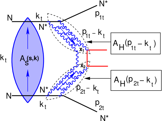
Figure 1: Central diffractive production in the two channel eikonal model in proton scattering due to pomeron exchange.

$A_{H}(b)$ is the hard pomeron amplitude in impact parameter space $b$ shown in Fig. 1. The amplitude $A_{H}\left(b\right)$ for hard pomeron exchange can be calculated in perturbative QCD, and is responsible for the production of two gluon jets, with BFKL ladder gluons between them (see Fig. 1). In this model [5], the hard pomeron in Fig. 1 emits the Higgs. $A_{H}(b)$ is given in the impact parameter $b$ representation by the expression [5]

$$A_{H}(b)=\frac{1}{\pi{}R_{H}^{2}}e^{-\frac{b^{2}}{R_{H}^{2}}}$$ (1.3)

$R_{H}^{2}=7.2GeV^{-2}$. As shown in Fig. 1, $A_{H}(b_{1})$ and $A_{H}(b_{2})$ denote the hard pomeron amplitude above and below the Higgs signal respectively. The contribution $A_{s}$, shown in Fig. 1, denotes the soft pomeron amplitude. $\left(\,1-A_{s}\right)\,$ includes all possible initial state interactions due to the exchange and interaction of soft Pomerons. $\left(\,1-A_{s}\right)\,$ also includes the possibility that the two initial nucleons in Fig. 1, do not interact at all.

The survival probability was found to be 5 - 6 $\%$ for the single channel model. In the two channel model, the survival probability here is $2.7\%{}$ at the LHC energy of $\sqrt{s}=14000$ $GeV$. The upper bound for the survival probability, in the constituent quark model (CQM), was found to be $6.0\%{}\pm{}0.1\%{}$ at the LHC energy. This is almost the same as the survival probability found in the single channel model. The two upper bounds, intercept at an energy just above the typical LHC energy. This suggests, that the upper bound for the survival probability, should be $2\%{}-3\%{}$ for measurements at the LHC.

The first attempt to estimate the contribution of hard (semi - hard) processes to the value of the survival probability, was made by Bartels, Bondarenko, Kutak and Motyka in [6]. They considered the contribution of this ”fan” pomeron diagram, to the value of the survival probability, and found that this contribution is rather large. Namely, the value ranges from $3.17\%\,$ for $\alpha_{s}=0.15$, to $1.6\%$ for $\alpha_{s}=0.25$, (where $\alpha_{s}$ is the QCD coupling).

The aim of this paper, is to calculate the BFKL pomeron (see Fig. 4), and the first enhanced diagram for the BFKL pomeron (see Fig. 6). These calculations are in the symmetric QCD dipole approach. Because in proton proton scattering, there is no reason to assume that the mean field approximation, based on the ”fan” diagram, can work. The ratio of the two contributions of Fig. 4 and Fig. 6 are calculated, and used to estimate the value of the survival probability.

This paper is organised in the following way. In section 2, the coupling of the BFKL pomeron to the colour dipole (section 2.1), and the triple pomeron vertex (section 2.2), are calculated in the momentum representation. Using these results, the BFKL pomeron amplitude shown in Fig. 4 is calculated (section 2.3), and the first enhanced diagram shown in Fig. 6, is calculated (section 2.4).

Section 3 is devoted to the survival probability, estimated in the QCD dipole approach. The ratio of the two contributions of Fig. 4 and Fig. 6 is calculated, which is used to estimate the value of the survival probability (section 3.2). It turns out, that this ratio is not small, and indicates the importance of taking into account all enhanced diagrams. Therefore, in section 3.3, all enhanced diagrams are summed in the toy model (see Ref.[7]). The fact that the two dipoles have different sizes is neglected. From the calculation of the ratio of Fig. 4 and Fig. 6, the value of the parameter $d$ of this model is determined, (d is the low energy amplitude for one pomeron exchange). Using this parameter, the value of the survival probability was estimated as the ratio of the diffractive Higgs production in this model, and Higgs production in one parton shower (for single pomeron exchange). It turns out that the survival probability is rather small.

In the conclusion, the results for the value of the survival probability is presented. A discussion is given on the dependence of the value of the survival probability, on the choice of intercept of the BFKL pomeron. The significance of higher order hard rescattering contributions to the survival probability, is also discussed.

2 The conformal eigenfunctions of the vertex operator and the triple pomeron vertex

All calculations are carried out in the momentum representation, and the strategy and notation of Ref. [10] is closely followed. Firstly, the pomeron coupling to the QCD colour dipole is introduced (see Fig. 2) in the momentum representation. Secondly, an explicit expression for the triple pomeron vertex (see Fig. 3) is derived. Using both these formulae, the BFKL pomeron (Fig. 4), and the first enhanced diagram (Fig. 6), are calculated in the symmetric QCD dipole approach.

2.1 The BFKL pomeron vertex function

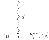
Figure 2: The vertex of interaction of Pomeron with the dipole.

The vertex coupling the BFKL pomeron to the couple dipole is illustrated in Fig. 2. Here, $\vec{q}$ is the momentum transferred along the pomeron, and $\vec{x}_{12}$ is the transverse size of the dipole. In the notation of Refs. [8, 9] , the eigenfunctions for the vertex in coordinate space are defined as

$$E^{n,\nu}\left(\,x_{01},x_{20}\right)=\left(-1\right)^{n}\left(\frac{x_{10}x_{20}}{x_{12}}\right)^{\gamma-\frac{1}{2}}\left(\frac{\bar{x}_{10}\bar{x}_{20}}{\bar{x}_{12}}\right)^{\bar{\gamma}-\frac{1}{2}}$$ (2.1.1)

where $x_{ij}=x_{i}-x_{j}$ and $x_{i}$ are the transverse coordinates. The conformal dimensions are defined as

$$\gamma=\frac{n}{2}-i\nu \bar{\gamma}=-\frac{n}{2}-i\nu$$ (2.1.2)

$n$ is the conformal spin, and is an integer. The energy levels of the pomeron are the BFKL eigenvalues given by [8]

$$\omega(n,\nu)\,=\bar{\alpha}_{s}\,\chi\left(\,\gamma\right)\,=\bar{\alpha}_{s}\,\left(\,2\psi\left(\,1\right)\,-\psi\left(\,\gamma\right)\,-\psi\left(\,1-\gamma\right)\,\right)\,$$ (2.1.3)

where in this paper the notation

$$\bar{\alpha}_{s}\,=\,\frac{\alpha_{s}\,N_{c}}{\pi}$$ (2.1.4)

is used, and where $\psi(f)=d\ln\Gamma(f)/df$ and $\Gamma(f)$ is the Euler gamma function. Since the only intercept $\omega(n=0,\nu)$ is positive at high energies, the contribution with $n\neq 0$ can be neglected. Lipatov in Ref. [8] introduces the following mixed representation of the vertex.

$$E^{n,\nu}_{q}\left(\vec{x}\right)=\frac{2\pi^{2}}{b_{n,\nu}}\frac{1}{|\vec{x}|}\int{}d^{2}Re^{i\vec{q}\cdot\,\vec{R}}E^{n,\nu}\left(\,R+\frac{x}{2},R-\frac{x}{2}\right)$$ (2.1.5)

where [8]

$$b_{n,\nu}=\frac{2^{4i\nu}\pi^{3}}{\frac{n}{2}-i\nu}\frac{\Gamma\left(\frac{n}{2}-i\nu+\frac{1}{2}\right)\Gamma\left(\frac{n}{2}+i\nu\right)}{\Gamma\left(\frac{n}{2}+i\nu+\frac{1}{2}\right)\Gamma\left(\frac{n}{2}-i\nu\right)}$$ (2.1.6)

A more convenient expression of Eq. (2.1.5) for the vertex was calculated in Ref. [9] and is given as

$$E^{n,\nu}_{q}\left(x_{12}\right)\,\,= \,\left(\,qq^{\ast}\right)\,^{i\nu}\,2^{-6\,i\,\nu}\,\Gamma^{2}(1-i\nu)\,\times$$

$$\,\left(J_{\gamma}\left(\frac{q^{*}\,x_{12}}{4}\right)\,J_{\tilde{\gamma}}\left(\frac{q\,x^{*}_{12}}{4}\right)\,\,-\,\left(\,-1\right)\,^{n}\,J_{-\gamma}\left(\frac{q^{*}\,x_{12}}{4}\right)\,J_{-\tilde{\gamma}}\left(\frac{q\,x^{*}_{12}}{4}\right)\right)$$

where $J_{\gamma}$ are the Bessel functions of the first kind. In Eq. (2.1), $q$ and $q^{\ast}$ are the components of the momentum $\vec{q}$ transferred along the pomeron, in the complex representation. That is

$$|\,q|\, = q\,q^{\ast}$$

$$\mbox{where}\,\,\,\,\,\,\,\,\,\,\,q = q_{x}+iq_{y}\,\,\,\,\,\,\,\,\,\,\,\,\,q^{\ast}\,=\,q_{x}-iq_{y}$$ (2.1.8)

In order to work in the momentum representation when calculating the single pomeron amplitude (Fig. 4), and the first enhanced diagram (Fig. 6), it is necessary to express the vertex function explicitly in the momentum representation. In Ref.[10] it was shown that in the momentum representation, the vertex function is given by the following Fourier transform

$$E\left(\vec{p},\vec{q};\gamma\right)\,=\frac{b_{n,\nu}}{2\pi^{2}}\int{}\frac{dx{}}{\sqrt{x{}}}\exp{}\left(-\frac{ip^{\ast}x{}}{2}\right)\int{}\frac{dx^{\ast}}{\sqrt{x^{\ast}}}\exp{}\left(-\frac{ix^{\ast}p}{2}\right)E^{n,\nu}_{q}\left(x{}\right)$$ (2.1.9)

Here $\vec{p}$ denotes the momentum which is the conjugate variable of the dipole size $x_{12}$. The complex representation, to express the vector $\vec{p}$ in terms of its complex components $p$ and $p^{\ast}$ (see Eq. (2.1.8)), is used in Eq. (2.1.9). In Ref. [10], this integral is written in the following factorised form

$$E\left(\vec{p},\vec{q};\gamma\,\right) = \frac{b_{n,\nu}}{2\pi^{2}}(q^{2})^{-i\nu}\,2^{-6\,i\,\nu}\,\Gamma^{2}(1-i\nu)\,\left(\,\tilde{E}(p,q;\tilde{\gamma})\tilde{E}(p^{*},q^{*};\gamma)-\tilde{E}(p,q;-\tilde{\gamma})\tilde{E}(p^{*},q^{*};-\gamma)\right)$$ (2.1.10)

where

$$\tilde{E}(p^{*},q^{*};\gamma)=\int\frac{dx}{\sqrt{x}}J_{\tilde{\gamma}}\left(\frac{q^{*}x}{4}\right)\,e^{-\frac{i}{2}p^{*}x} \tilde{E}(p,q;\tilde{\gamma})=\int\frac{dx^{*}}{\sqrt{x^{*}}}J_{\gamma}\left(\frac{qx^{*}}{4}\right)\,e^{-\frac{i}{2}px^{*}}$$ (2.1.11)

At this point, it is assumed that $n=0$, and hence $\gamma=\tilde{\gamma}=-i\nu$ (see Eq. (2.1.2)). This is because the only intercept $\omega\left(\,n=0,\nu\right)\,$ is positive at high energies (see Eq. (2.1.3)), so the contribution $n\neq\,0$ is neglected from now onwards. Let $\tilde{E}(p^{*},q^{*};\gamma)$ and $\tilde{E}(p,q;\tilde{\gamma})$ be denoted as $\tilde{E}(p^{*},q^{*};\nu)$ and $\tilde{E}(p,q;\nu)$ for $n=0$. After integration over $x$ and $x^{\ast}$, the expressions for $\tilde{E}\left(\,q,p;\nu\right)\,$ and $\tilde{E}\left(\,q^{\ast},p^{\ast};\nu\right)\,$ are found to be [10]

$$\tilde{E}(p,q;\nu) = \left(\,\frac{q}{8}\right)^{-i\nu}\left(\,-1\right)^{-i\nu}\,i^{i\nu+\frac{1}{2}}2^{\frac{3}{2}-i\nu}p^{i\nu-\frac{1}{2}}\frac{\Gamma\left(\,\frac{1}{2}-i\nu\right)}{\Gamma\left(\,1-i\nu\right)\,}\,\,\,$$

$$\times\, \,\,\,\,{}_{2}F_{1}\left(\,\frac{1}{4}-\frac{1}{2}i\nu\,,\frac{3}{4}-\frac{1}{2}i\nu\,,1-i\nu\,,\frac{q^{2}}{4p^{2}}\right)\,$$

$$\tilde{E}(p^{*},q^{*};\nu) = \left(\,\frac{q^{\ast}}{8}\right)^{-i\nu}\left(\,-1\right)^{-i\nu}\,i^{i\nu+\frac{1}{2}}2^{\frac{3}{2}-i\nu}\left(\,p^{\ast}\right)\,^{i\nu-\frac{1}{2}}\frac{\Gamma\left(\,\frac{1}{2}-i\nu\right)}{\Gamma\left(\,1-i\nu\right)\,}\,\,\,$$

$$\times\, \,\,\,\,{}_{2}F_{1}\left(\,\frac{1}{4}-\frac{1}{2}i\nu\,,\frac{3}{4}-\frac{1}{2}i\nu\,,1-i\nu\,,\frac{\left(\,q^{\ast}\right)\,^{2}}{4\left(\,p^{\ast}\right)\,^{2}}\right)\,$$

Hence, using Eq. (LABEL:TI) and the expression for $b_{n=0,\nu}$ in Eq. (2.1.6), the RHS of Eq. (2.1.10) can be written in the explicit form as

$$\,E\left(\vec{p},\vec{q};\nu\right)\,\, = -\frac{2^{2+2i\nu}\left(\,p^{2}\right)\,^{i\nu-\frac{1}{2}}\pi^{2}}{\nu}\frac{\Gamma^{2}\left(\,\frac{1}{2}-i\nu\right)\,}{\Gamma^{2}\left(\,\frac{1}{2}+i\nu\right)\,}\frac{\Gamma\left(\,i\nu\,\right)\,}{\Gamma\left(\,-i\nu\right)\,}$$

$$\times\, {}_{2}F_{1}\left(\,\frac{1}{4}-\frac{1}{2}i\nu\,,\frac{3}{4}-\frac{1}{2}i\nu\,,1-i\nu\,,\frac{q^{2}}{4p^{2}}\right)\,_{2}F_{1}\left(\,\frac{1}{4}-\frac{1}{2}i\nu\,,\frac{3}{4}-\frac{1}{2}i\nu\,,1-i\nu\,,\frac{\left(\,q^{\ast}\right)\,^{2}}{4\left(\,p^{\ast}\right)\,^{2}}\right)\,$$

$$+ \frac{2^{2-6i\nu}\left(\,p^{2}\right)\,^{i\nu-\frac{1}{2}}\pi^{2}}{\nu}\left(\,\frac{q^{2}}{p^{2}}\right)^{2i\nu}\,\,\,\frac{\Gamma^{2}\left(\,1-i\nu\right)\,\Gamma\left(\,i\nu\right)\,}{\Gamma^{2}\left(\,1+i\nu\right)\,\Gamma\left(\,-i\nu\right)\,}\,\,\,\,$$

$$\times\, {}_{2}F_{1}\left(\,\frac{1}{4}+\frac{1}{2}i\nu\,,\frac{3}{4}+\frac{1}{2}i\nu\,,1+i\nu\,,\frac{q^{2}}{4p^{2}}\right)\,_{2}F_{1}\left(\,\frac{1}{4}+\frac{1}{2}i\nu\,,\frac{3}{4}+\frac{1}{2}i\nu\,,1+i\nu\,,\frac{\left(\,q^{\ast}\right)\,^{2}}{4\left(\,p^{\ast}\right)\,^{2}}\right)\,$$

where $E\left(\vec{p},\vec{q};n=0,\gamma\right)$ is written as $E\left(\vec{p},\vec{q};\nu\right)$. For single pomeron exchange, (see Fig. 4), the conformal spin $\nu$ has opposite signs at the two vertices at the ends of the pomeron. In section 2.3 when Fig. 4 is calculated, it is assumed that $\vec{q}=0$ to simplify the calculation. Hence, from Eq. (2.1), the product of two vertices, (for $\vec{q}=0$) takes the form

$$E\left(\vec{p},\vec{q}=0;\,\nu\,\right)\,E\left(\vec{p},\vec{q}=0;\,-\nu\,\right)\,= \frac{1}{\nu^{2}}\frac{16\pi^{4}}{p^{2}}$$ (2.1.14)

2.2 The triple pomeron vertex

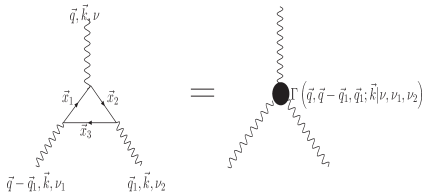
Figure 3: The triple Pomeron vertex.

In this subsection the triple pomeron vertex, illustrated in Fig. 3 is calculated explicitly in the momentum representation. It is defined in Refs. [9, 11, 12] as an integral over the centre of mass position vectors $\left(\,x_{01},x_{02},x_{03}\right)\,$, and the conformal dimensions $(\gamma,\gamma_{1},\gamma_{1})$ as

$$G_{3P}\left(\vec{q},\vec{k},n=0,\gamma,\gamma_{1},\gamma_{2}\right)\,\, = \,\,G_{3P}\left(\vec{q},\vec{k},\nu,\nu_{1},\nu_{2}\right)\,\,$$

$$= \,\,\int{}\frac{d^{2}x_{10}d^{2}x_{20}d^{2}x_{30}}{x_{12}x_{23}x_{31}}E^{n,\nu}_{q}\left(\,x_{10},x_{20}\right)\,E^{n,\nu_{1}}_{k}\left(\,x_{20},x_{30}\right)\,E^{n,\nu_{2}}_{q-k}\left(\,x_{30},x_{10}\right)$$

To calculate the triple pomeron vertex explicitly, the mixed representation of Lipatov in Ref.[8] is used for the vertex eigenfunctions $E^{n,\nu}_{q}$ (see Eq. (2.1.5)). Note that to simplify the calculation of the first enhanced diagram of Fig. 6, it is assumed that $\vec{q}=0$ for the momentum transferred along the pomeron, above and below the pomeron loop. Hence, the triple pomeron vertex shown in Fig. 3 is calculated for $\vec{q}=0$. In Ref.[12] this mixed representation was used in the definition of Eq. (2.2) to give the expression

$$G_{3P}(\vec{q}=0,\vec{k},\nu{},\nu_{1},\nu_{2})=\frac{1}{2\pi{}}\int\frac{d^{2}x_{01}}{x_{01}^{2}}x_{01}^{-2i\nu-1}e^{\frac{i\vec{k}\cdot\,\vec{x}_{01}}{2}}\int{}d^{2}x_{2}\frac{x_{01}^{2}}{x_{12}^{2}x_{02}^{2}}x_{02}^{2i\nu_{1}+1}E_{k}^{n,\nu_{1}}(x_{02})x_{12}^{2i\nu_{2}+1}E_{-k}^{n,\nu_{2}}(x_{12})$$ (2.2.2)

It is also assumed that $\nu_{1}=\nu_{2}=0$ in evaluating the expression of Eq. (2.2.2) for the triple pomeron vertex, for the following reason. When evaluating the integrals over $\nu_{1}$ and $\nu_{2}$, for the expression of Fig. 6, (see Eq. (2.4.2)), one expands the BFKL functions $\omega\left(\nu_{1}\right)\,$ and $\omega\left(\,\nu_{2}\right)\,$ around the saddle point $\nu_{1}=\nu_{2}=0$ (see Eq. (A-2-9)), which gives the largest contribution to the integration. In the appendix, the integral of Eq. (2.2.2) is evaluated to give the triple pomeron vertex as an explicit expression in the momentum representation in Eq. (A-1-14) as

$$G_{3P}(\vec{q}=0,\vec{k},\nu,\nu_{1}\rightarrow\,0,\nu_{2}\rightarrow\,0,)\,\,\,=\,\,\,k^{i\nu-\frac{1}{2}}\frac{2^{-2i\nu}}{4\nu_{1}\nu_{2}\pi}\frac{\Gamma^{3}\left(\,\frac{1}{2}-i\nu\right)\,\Gamma^{2}\left(\,i\nu\right)\,}{\Gamma\left(\,\frac{1}{2}+i\nu\right)\,}$$ (2.2.3)

2.3 The single pomeron amplitude

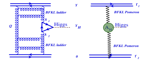
Figure 4: Central diffractive production in colour dipole scattering due to single pomeron exchange.

In this subsection the single pomeron amplitude with Higgs production shown in Fig. 4 is calculated. The two dipoles are separated by a rapidity gap $Y$, and they have transverse sizes $r_{1}=x_{12}$ and $r_{2}=x_{12}^{\prime}$. The momenta conjugate to the dipole sizes are $\vec{p}_{1}$ and $\vec{p}_{2}$, and $\vec{q}$ is the momentum transferred along the pomeron. For simplicity it is assumed that $\vec{q}=0$. The single pomeron amplitude with Higgs production, in the QCD dipole approach is denoted $M_{Higgs}\left(\,n=1\,,\,Y\right)\,$, where $Y$ is the rapidity gap between the two incoming protons, and $n=1$ denotes the single pomeron exchanged between the two protons. In this notation, the single pomeron amplitude, with Higgs production of Fig. 4, has the expression [8, 9, 13, 14]

$$M_{Higgs}\left(\,n=1\,,\,Y\right)\,\,=\,\,P^{BFKL}(\vec{p}_{1},\vec{p}_{2},Y,\vec{q}=0)\,A_{H}\left(\,\delta\,Y_{H}\right)\,$$ (2.3.1)

where $P^{BFKL}(\vec{p}_{1},\vec{p}_{2},Y,\vec{q}=0)\,$ is the single pomeron amplitude given by the expression

$$P^{BFKL}(\vec{p}_{1},\vec{p}_{2},Y,\vec{q}=0)=\frac{\alpha_{s}^{2}}{4}\int{}\frac{d\nu{}}{2\pi{}i}\mathcal{D}(\nu{})e^{\omega(\nu{})}E\left(\,\vec{p}_{1},\vec{q}=0,\nu{}\right)\,E\left(\,\vec{p}_{2},\vec{q}=0,-\nu{}\right)\,$$ (2.3.2)

and where $A_{H}\left(\,\delta\,Y_{H}\right)\,$ denotes the subprocess contribution which produces the Higgs, such as the quark triangle subprocess of Fig. 5. The typical rapidity window, which the Higgs Boson occupies is $\delta\,Y_{H}\,=\,\ln\left(\,\frac{M_{H}^{2}}{4m^{2}}\right)\,$, where $m$ is the mass of the proton. The simplest subprocess with the largest contribution for Higgs production in the standard model, is the quark triangle shown in Fig. 5. After the subprocess amplitude of Fig. 5 is contracted with the gluon propagators, the expression for the contribution of the quark triangle shown in Fig. 5 is given by [15, 16]

Figure 5: Quark triangle subprocess for Higgs production.

$$A_{H}\left(\,\delta\,Y_{H}\right)\,\,=\,\,A\left(\,M_{H}^{2}\right)\,\,\left(\,\vec{k}_{1}\cdot\,\vec{k}_{2}\,\right)\,\,$$ (2.3.3)

where the factor $A\left(\,M_{H}^{2}\right)\,$ has the value [17, 18, 19, 20]

$$A\left(\,M_{H}^{2}\right)\,=\,\frac{2}{3}\left(\frac{-\alpha{}_{s}\left(M_{H}^{2}\right)\left(\sqrt{2}G_{F}\right)^{\frac{1}{2}}}{\pi{}}\right)$$ (2.3.4)

where $G_{F}$ is the Fermi coupling. $D\left(\nu\right)$ appearing in the single pomeron amplitude of Eq. (2.3.2) is given by

$$\mathcal{D}(\nu{})=\frac{\nu{}^{2}}{\left(\,\nu{}^{2}+\frac{1}{4}\right)\,^{2}}$$ (2.3.5)

$\omega(n=0,\nu{})$ is the solution to the BFKL equation defined in Eq. (2.1.3), where in the high energy limit one takes $n=0$. From now on the notation $\omega(n=0,\nu{})=\omega\left(\,\nu\right)$ is used. Assuming that the conjugate momenta $\vec{p}_{1}$ and $\vec{p}_{2}$ of the two scattering dipoles in Fig. 4 are equal in magnitude, Eq. (2.1.14) can be used for the product of the two pomeron vertices. Hence, Eq. (2.3.5) can be written as

$$P^{BFKL}(\vec{p}_{1}=\vec{p}_{2}=\vec{p},Y,\vec{q}=0)=\frac{4\alpha_{s}^{2}\pi^{4}}{p^{2}}\int{}\frac{d\nu{}}{2\pi{}i}\frac{1}{\left(\,\frac{1}{4}+\nu^{2}\right)^{2}}\,e^{\omega(\nu{})Y}$$ (2.3.6)

The integration over $\nu$ can be evaluated at the saddle point $\nu=0$ of $\omega\left(\nu\right)$. In this way, the RHS of Eq. (2.3.6) becomes

$$P^{BFKL}(\vec{p}_{1}=\vec{p}_{2}=\vec{p},Y,\vec{q}=0) =\frac{32\alpha_{s}^{2}\pi^{3}}{p^{2}}\left(\,\frac{2\pi{}}{(\omega{}"(\nu{}=0)Y)}\right)^{\frac{1}{2}}\,e^{\omega{}(\nu{}=0)Y}$$ (2.3.7)

Hence, the final expression of Eq. (2.3.1) for the process of Fig. 4 reads

$$M_{Higgs}\left(\,n=1\,,\,Y\right)\, =\frac{32\alpha_{s}^{2}\pi^{3}}{p^{2}}\left(\,\frac{2\pi{}}{(\omega{}"(\nu{}=0)Y)}\right)^{\frac{1}{2}}\,e^{\omega{}(\nu{}=0)Y}\,A_{H}\left(\,\delta\,Y_{H}\right)\,$$ (2.3.8)

This is the expression for the single pomeron amplitude, including Higgs production, of Fig. 4. However, Eq. (2.3.8) is written in the approximation that $s=(p_{1}+p_{2})^{2}\,\gg\,M^{2}_{H}$ . Since we expect the Higgs mass to be large, we take into account the main correction due to this mass, namely, we make the following replacement.

$$e^{\omega{}(\nu{}=0)Y}\,\equiv\,\,\left(\frac{s}{m^{2}}\right)^{\omega(\nu=0)\,Y}\,\,\longrightarrow\,\,\left(\frac{1}{x_{1}\,x_{2}}\right)^{\omega(\nu=0)\,Y}\left(\frac{4\,s}{M^{2}_{H}}\right)^{\omega(\nu=0)\,Y}\,\,\equiv\,\,e^{\omega{}(\nu{}=0)\,\left(\,Y-\ln(M^{2}_{H}/4m^{2})\right)\,}$$ (2.3.9)

where $m$ is the mass of proton., $x_{1}$ and $x_{2}$ are equal to $k^{2}_{1}/s_{1}$ and $k^{2}_{2}/s_{2}$ (see Fig. 4) with $s_{1}=(p_{1}+k_{1})^{2}$ and $s_{2}=(p_{2}+k_{2})^{2}$). Using the well known kinematic relation $s_{1}\,s_{2}\,=\,M^{2}_{H}\,s$ and since $k^{2}_{1}\,=\,k^{2}_{2}\,=\,M^{2}_{H}/2$ (see Ref. [28] for example). Finally, Eq. (2.3.8) looks as follows

$$M_{Higgs}\left(\,n=1\,,\,Y\right)\, =\frac{32\alpha_{s}^{2}\pi^{3}}{p^{2}}\left(\,\frac{2\pi{}}{(\omega{}"(\nu{}=0)Y)}\right)^{\frac{1}{2}}\,e^{\omega{}(\nu{}=0)\,(Y\,-\,\ln(M^{2}_{H}/4m^{2}))}\,A_{H}\left(\,\delta\,Y_{H}\right)\,$$ (2.3.10)

As one can see in Eq. (2.3.10) the single Pomeron exchange does not depend on the value of Higgs boson rapidity ($Y_{H}$) but depends on $\delta Y_{H}=\ln(M^{2}_{H}/4m^{2})$ which characterizes the window in rapidity occupied by the heavy Higgs boson.

2.4 The first enhanced amplitude

In this subsection the amplitude for the first enhanced amplitude, with Higgs production shown in Fig. 6, is calculated. The pomeron loop is between the two rapidity values $Y_{1}$ and $Y_{2}$. Hence, one needs to integrate over these two rapidity values. There is also an integral to evaluate, over the unknown momentum $\vec{k}$ in the pomeron loop. The enhanced diagram with Higgs production, in the QCD dipole approach is denoted $M_{Higgs}\left(\,n=2\,,\,Y\right)\,$, where $n=2$ denotes the splitting of the exchanged pomeron, into two branches forming the loop in Fig. 6. The amplitude of Fig. 6, is the first hard rescattering correction, to the single pomeron amplitude of Fig. 4. In this notation, first enhanced amplitude, with Higgs production of Fig. 6 is given by

$$M_{Higgs}\left(\,n=2\,,\,Y\right)\,\,=\,\,2\,P^{BFKL}_{enhanced}(\vec{p}_{1},\vec{p}_{2},Y,\vec{q})\,A_{H}\left(\,\delta\,Y_{H}\right)\,$$ (2.4.1)

where $P^{BFKL}_{enhanced}(\vec{p}_{1},\vec{p}_{2},Y,\vec{q})$ is the BFKL pomeron amplitude for the first enhanced one - loop diagram, which has the expression given below in Eq. (2.4.2). The factor of $2$ in Eq. (2.4.1), comes from adding the two identical contributions of Fig. 6, due to the two ways the Higgs is emitted from the two branches of the pomeron loop. In order to obtain the complete contribution of Fig. 6, both possibilities for Higgs production from the two branches of the loop must be considered separately, and added. $P^{BFKL}_{enhanced}(\vec{p}_{1},\vec{p}_{2},Y,\vec{q})$ is given by the expression (see Refs. [9, 13])

$$P^{BFKL}_{enhanced}(\vec{p}_{1},\vec{p}_{2},Y,\vec{q})= \,\,\,B\int\!d\nu\,d\nu^{\prime}d\nu_{1}d\nu_{2}d^{2}k{}\int^{Y}_{Y_{H}+\frac{1}{2}\delta Y_{H}\,}dY_{1}\int^{Y_{H}-\frac{1}{2}\delta Y_{H}}_{0}dY_{2}$$

$$\times\,E\left(\,\vec{p}_{1},\vec{q},\nu{}\right)\,\mathcal{D}\left(\,\nu\right)\,e^{\omega{}(\nu{})(Y-Y_{1})}G_{3P}(\nu,\nu_{1},\nu_{2},\vec{q}=0,\vec{k})$$

$$\times\,\mathcal{D}\left(\,\nu_{1}\right)\,\mathcal{D}\left(\,\nu_{2}\right)\,e^{(\omega(\nu_{1})+\omega(\nu_{2}))(Y_{1}-Y_{2})\,-\,\omega(\nu_{2})\,\ln(M^{2}_{H}/4m^{2})}\,G_{3P}(-\nu{}^{\prime},\nu_{1},\nu_{2},\vec{q}=0,\vec{k})$$

$$\times\,e^{\omega{}(\nu{}^{\prime})Y_{2}}E\left(\,\vec{p}_{2},\vec{q},-\nu{}^{\prime}\right)\,$$ (2.4.2)

$$\mbox{where}\,\,\,\,\,B= \,\,\,-\frac{\alpha_{s}^{4}\pi^{4}}{8}\left(\,\frac{\alpha_{s}\,N_{c}}{2\pi^{2}}\right)^{2}$$ (2.4.3)

where $Y_{H}$ is the rapidity of the Higgs boson. $Y_{H}$ here is considered equal to zero in the c.m. frame, restricting ourselves to the production of the Higgs boson at rest in the c.m. frame since it is the most likely experimental kinematic, and $\delta Y_{H}=\ln\left(M^{2}_{H}/4m^{2}\right)$ characterizes the rapidity window, occupied by the Higgs boson.

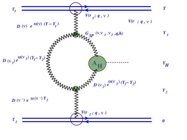
Figure 6: Central diffractive production in colour dipole scattering due to pomeron exchange with a hard rescattering correction.

Using the same assumptions as section 2.2, the integral over $\vec{k}$ in Eq. (2.4.2) is evaluated in the appendix with the result given in Eq. (A-1-17) as

$$\int\!d^{2}kG_{3P}(\nu,\nu_{1}\rightarrow\,0,\nu_{2}\rightarrow\,0,\vec{q}=0,\vec{k})G_{3P}(-\nu{}^{\prime},\nu_{1}\rightarrow\,0,\nu_{2}\rightarrow\,0,\vec{q}=0,\vec{k})$$ (2.4.4)

$$\xrightarrow{\nu_{1},\nu_{2}\rightarrow\,0} \frac{2^{2(i\nu{}^{\prime}-i\nu{})}}{8}\frac{\delta{}(\nu{}-\nu{}^{\prime})}{4\nu_{1}^{2}4\nu_{2}^{2}}\frac{\Gamma^{3}\left(\,\frac{1}{2}+i\nu{}^{\prime}\right)\,\Gamma^{3}\left(\,\frac{1}{2}-i\nu{}\right)\,\Gamma^{2}\left(\,-i\nu^{\prime}\right)\,\Gamma^{2}\left(\,i\nu\right)\,}{\Gamma\left(\,\frac{1}{2}-i\nu{}^{\prime}\right)\,\Gamma\left(\,\frac{1}{2}+i\nu{}\right)\,}$$

Note that the $\nu_{1}^{2}$ and $\nu_{2}^{2}$ in the denominator of Eq. (2.4.4) cancel with $\mathcal{D}\left(\,\nu_{1}\right)\,$ and $\mathcal{D}\left(\,\nu_{2}\right)\,$ in Eq. (2.4.2) (see Eq. (2.3.5)). When inserting Eq. (2.4.4) into the right hand side of Eq. (2.4.2), the delta function allows the integration over $\nu{}^{\prime}$ to be evaluated to give the result

$$P^{BFKL}_{enhanced}(\vec{p}_{1},\vec{p}_{2},Y,\vec{q}=0)= \,\,\,\frac{B\pi^{2}}{8}\int\!d\nu\,d\nu_{1}d\nu_{2}\int^{Y}_{Y_{H}+\frac{1}{2}\delta Y_{H}}dY_{1}\int^{Y_{H}-\frac{1}{2}\delta Y_{H}}_{0}dY_{2}$$

$$\times\,E\left(\,\vec{p}_{1},\vec{q},\nu{}\right)\,\mathcal{D}^{2}(\nu)e^{\omega(\nu)(Y-Y_{1}+Y_{2})}\frac{\Gamma{}^{2}\left(\,\frac{1}{2}-i\nu{}\right)\,\Gamma{}^{2}\left(\,\frac{1}{2}+i\nu{}\right)\,}{4\nu_{1}^{2}4\nu_{2}^{2}\nu{}^{2}\sin{}^{2}\left(i\nu{}\pi{}\right)}$$

$$\times\mathcal{D}(\nu_{1})\mathcal{D}(\nu_{2})e^{(\omega(\nu_{1})+\omega(\nu_{2}))(Y_{1}-Y_{2})\,\,-\,\,\omega(\nu_{2})\,\ln(M^{2}_{H}/4m^{2})}\,E\left(\,\vec{p}_{2},\vec{q},-\nu{}\right)\,$$ (2.4.5)

Now the integrals over $\nu$,$\nu_{1}$,$\nu_{2}$ and the two rapidity values $Y_{1}$ and $Y_{2}$ need to be evaluated. $Y_{1}$ and $Y_{2}$ are the upper and lower rapidity values for the pomeron loop in Fig. 6. The details of the integrations are given in the appendix in Eq. (A-2-3)-Eq. (A-2-11), and the final expression is given in Eq. (A-2-11) as

$$P^{BFKL}_{enhanced}(\vec{p}_{1},\vec{p}_{2},Y,\vec{q}=0)=$$ (2.4.6)

$$\frac{32\,B\pi^{8}\,}{\left(\,2\bar{\alpha}_{s}\right)^{5}p^{2}}\frac{\delta\,Y_{H}}{\omega"\left(\,\nu\,=0\right)\,}\left(\,\frac{\left(\,2\omega\left(\,\nu\,=0\,\right)\,\right)^{4}\,}{Y}-4\frac{\left(\,2\omega"\left(\,\nu\,=0\,\right)\,\right)^{3}}{Y^{2}}\right)\,\,e^{2\omega\left(\,\nu\,=0\,\right)\,\left(\,Y-\frac{1}{2}\,\ln\left(\,\frac{M_{H}^{2}}{4m^{2}}\right)\,\right)\,}\,$$

where the constant $B$ is given in Eq. (2.4.3). Therefore, the full expression for the diagram of Fig. 6 given by Eq. (2.4.1) takes the form

$$M_{Higgs}\left(\,n=2\,,\,Y\right)\,\,=\,$$

$$\frac{64\,B\pi^{8}\,}{\left(\,2\bar{\alpha}_{s}\right)^{5}p^{2}}\frac{\delta\,Y_{H}}{\omega"\left(\,\nu\,=0\,\right)\,}\left(\,\frac{\left(\,2\omega\left(\,\nu\,=0\,\right)\,\right)^{4}\,}{Y}-4\frac{\left(\,2\omega"\left(\,\nu\,=0\,\right)\,\right)^{3}}{Y^{2}}\right)\,\,e^{2\omega\left(\,\nu\,=0\,\right)\,\left(\,Y-\frac{1}{2}\,\ln\left(\,\frac{M_{H}^{2}}{4m^{2}}\right)\,\right)\,}\,A_{H}\left(\,\delta\,Y_{H}\right)\,$$

3 The survival probability in diffractive Higgs production in colour dipole scattering due to pomeron exchange

3.1 The definition of survival probability

In this section the survival probability of large rapidity gaps, in diffractive Higgs production is calculated, using the ratio of Fig. 4 and Fig. 6 (see and Eq. (2.3.8) and Eq. (2.4)). To guarantee that there will still be a large rapidity gap (LRG) between the protons after scattering, all hard rescattering corrections, that could give terms filling up the LRG, must be taken into account. The survival probability, is the probability to just have the exclusive Higgs production shown in Fig. 4, and not to have any higher order hard rescattering corrections, such as the first enhanced diagram of Fig. 6. In other words , the survival probability is the ratio of the calculated cross section for the Higgs boson production to the one form the one pomeron exchange. Hence, the survival probability of the LRG, is calculated by subtracting the sum over all hard rescattering amplitudes from the single pomeron amplitude of Fig. 4, and dividing the result by the single pomeron amplitude of Fig. 4 itself, to obtain the correctly normalised survival probability. Therefore, the survival probability is defined as

$$<\,|\,S^{2}|\,>\,=\,\frac{M_{Higgs}\left(\,n=1\,,\,Y\right)\,-\sum^{\infty}_{n=2}\,\left(\,-1\right)^{n}\,M_{Higgs}\left(\,n\,,\,Y\right)\,}{M_{Higgs}\left(\,n=1\,,\,Y\right)\,}$$ (3.1.1)

where $M_{Higgs}\left(\,n\,,\,Y\right)\,$ is the $n^{th}$ order hard rescattering correction. For example, in the case of $n=2$, the first hard rescattering correction $M_{Higgs}\left(\,n=2\,,\,Y\right)\,$ is the contribution of the first enhanced diagram of Fig. 6, which has $2$ pomeron branches, forming the pomeron loop. In general, $M_{Higgs}\left(\,n\,,\,Y\right)\,$ is the contribution given by the diagram which has $n$ pomeron branches. In calculating the survival probability, if only the first enhanced diagram is taken into account, and corrections of the order $n=3$ and higher are ignored, then the formula of Eq. (3.1.1) reduces to

$$<\,|\,S^{2}|\,>\,=\,\frac{M_{Higgs}\left(\,n=1\,,\,Y\right)\,-\,M_{Higgs}\left(\,n=2\,,\,Y\right)\,}{M_{Higgs}\left(\,n=1\,,\,Y\right)\,}\,=\,1-\frac{M_{Higgs}\left(\,n=2\,,\,Y\right)\,}{M_{Higgs}\left(\,n=1\,,\,Y\right)\,}$$ (3.1.2)

The ratio $\frac{M_{Higgs}\left(\,n=2\,,\,Y\right)\,}{M_{Higgs}\left(\,n=1\,,\,Y\right)\,}$ is calculated in the next subsection, in the symmetric QCD dipole approach (see Eq. (3.2.4) in section 3.2). It turns out that this ratio is not small and, therefore, all enhanced diagrams need to be taken into account. Using the toy model suggested by Mueller in Ref.[7], all enhanced diagrams are taken into account in the Mueller - Patel- Salam - Iancu (MPSI) approach (see Refs.[21, 22, 23]). The formula for the scattering amplitude in this model was suggested by Kovchegov in Ref. [24].

3.2 The QCD dipole approach

The survival probability of large rapidity gaps, in diffractive Higgs production in the QCD dipole approach, is the probability for the exclusive Higgs production of Fig. 4, with a large rapidity gap between the Higgs signal and the two emerging dipoles. To calculate the survival probability, all hard rescattering corrections which could fill up the large rapidity gaps must be subtracted from the single BFKL Higgs amplitude $M_{Higgs}\left(\,n=1\,,\,Y\right)\,$, and the result must be divided by $M_{Higgs}\left(\,n=1\,,\,Y\right)\,$. If only the first enhanced rescattering correction $M_{Higgs}\left(\,n=2\,,\,Y\right)\,$ is taken into account, then the survival probability in the symmetric QCD dipole approach is estimated as

$$<|S^{2}|>\,=\,\frac{M_{Higgs}\left(\,n=1\,,\,Y\right)\,-M_{Higgs}\left(\,n=2\,,\,Y\right)\,}{M_{Higgs}\left(\,n=1\,,\,Y\right)\,}\,\,=\,1\,-\,\frac{M_{Higgs}\left(\,n=2\,,\,Y\right)\,}{M_{Higgs}\left(\,n=1\,,\,Y\right)\,}$$ (3.2.1)

where the amplitudes $M\left(\,n=1\,,\,Y\,\right)\,$ and $M\left(\,n=2\,,\,Y\right)$ have been calculated in Eq. (2.3.8) and Eq. (2.4), respectively. Using the results of Eq. (2.3.8) and Eq. (2.4), then the ration $\frac{M\left(\,n=2\,,\,Y\,\right)\,}{M\left(\,n=1\,,\,Y\,\right)\,}$ appearing in Eq. (3.2.1) is found to have the expression

$$\frac{M_{Higgs}\left(\,n=2\,,\,Y\right)\,}{M_{Higgs}\left(\,n=1\,,\,Y\right)\,}=$$

$$\frac{2\,B\pi^{5}\,}{\alpha_{s}^{2}\,\left(\,2\bar{\alpha}_{s}\right)^{5}}\frac{\delta\,Y_{H}}{\omega\,"\left(\,\nu\,=0\,\right)\,}\left(\,\frac{\left(\,2\omega\left(\,\nu=\,0\right)\,\right)^{4}}{Y}-\,4\,\frac{\left(\,2\omega\left(\,\nu\,=\,0\right)\,\right)^{3}}{Y^{2}}\right)\,\left(\,\frac{\omega"\left(\,\nu\,=0\,\right)\,Y}{2\pi}\right)^{\frac{1}{2}}e^{\omega\left(\,\nu\,=0\,\right)\,Y}$$

where the constant $B$ is given in Eq. (2.4.3). Here a typical value for $\alpha{}_{s}$, which depends on the mass of the $Z$ particle, is used. It is expected that the Higgs will be produced with a mass of approximately $100$ $GeV$, which would give a value for the strong coupling constant $\alpha{}_{s}\sim{}0.12{}$. This corresponds to a $Z$ particle mass [25], of $M_{Z}=90.8\pm{}0.6$ $Gev$.
The following values are to be found in Ref. [25] and Ref. [26], for the strong coupling and the BFKL function.

$$\alpha_{s}=0.12 \omega{}(\nu{}=0)=\bar{\alpha}_{s}4\ln 2 \frac{1}{2}\omega{}"(\nu{}=0)=14\bar{\alpha}_{s}\,\zeta(3) \zeta(3)\cong{}1.202$$ (3.2.3)

Assuming that the rapidity gap $Y$ at the LHC is 19, and using the numerical values given in Eq. (3.2.3), the right hand side of Eq. (3.2) then yields following.

$$\frac{M\left(\,n=2\,,\,Y\,\right)\,}{M\left(\,n=1\,,\,Y\right)\,}=2.8\,\,\,e^{\omega{}(\nu{}=0)Y}$$ (3.2.4)

This value is not small and increases with energy. Therefore, it shows that all enhanced diagrams have to be taken into account. In the next section all enhanced diagrams are summed in the toy model.

3.3 The toy model approach

In this subsection, the survival probability is calculated taking into account all enhanced diagrams. The toy model proposed by Mueller in Ref. [7], is a model for describing pomeron exchange in onium - onium scattering. In the toy model, the dipole wave function of an onium is described by the generating functional for dipoles ([7]) $Z(Y,[u])$:

$$Z\left(Y\,-\,Y_{0};\,[u]\right)\,\,\equiv\,\,$$ (3.3.1)

$$\equiv\,\,\sum_{n=1}\,\int\,\,P_{n}\left(Y;\,r_{1},b_{1},\,r_{2},b_{2},\dots,r_{i},b_{i},\dots,r_{n},b_{n}\right)\,\,\prod^{n}_{i=1}\,u(r_{i},b_{i})\,d^{2}\,r_{i}\,d^{2}\,b_{i}$$

Here, $P_{n}$ are the probabilities to find dipoles with sizes $r_{i}$ and impact parameters $b_{i}$ at rapidity Y and $u(x_{01},b)$ is an arbitrary function of the dipole of transverse size $x_{01}$, at impact parameter $b$ . In the toy model which we are going to consider here we neglect the dependence of $u$ on the size of dipoles and their impact parameters(see Ref. [7]) . In this model $Z(x_{01},b,Y,u)$ degenerates to the generating function and obeys the following evolution equation (see Ref. [7])

$$\frac{dZ\left(\,Y,u\right)\,}{dY}=\Delta\,Z^{2}\left(Y,u\right)\,-\Delta\,Z\left(Y,u\right)\,$$ (3.3.2)

where $\Delta\,$ is the pomeron intercept. In section 2.3 and section 2.4, the pomeron intercept can be taken to be the BFKL intercept $\Delta\,=\,\omega\left(\,\nu\,=\,0\right)\,$ to provide a matching with the BFKL Pomeron calculus. The initial condition for Eq. (3.3.2) is given by

$$Z(Y=0,u)=u\,$$ (3.3.3)

The solution of the toy model Eq. (3.3.2), which satisfies the initial condition of Eq. (3.3.3) is [7, 24]

$$Z(Y,u)=\frac{u\,}{u\,+(1-u)\,e^{\Delta\,Y}}$$ (3.3.4)

Eq. (3.3.4) gives the sum over all ”fan” diagrams. To generalise this result to the sum over all essential enhanced diagrams, the MPSI approximation is used to sum over all diagrams, with pomeron loops larger than $\frac{Y}{2}$. In Ref.[24], the forward scattering amplitude in the MPSI approximation was written and has the form

$$D(Y\,,\,d)=1-\exp\left(\,-d\frac{d{}^{2}}{d{}u\,d{}v}\right)\,Z\left(\frac{Y}{2},u\right)Z\left(\frac{Y}{2},v\right)|_{u=1,v=1}$$ (3.3.5)

where $d$ is the dipole amplitude $(0<\,d<\,1)$ at low energy. Substituting for $Z\left(Y,u\right)$, the right hand side of Eq. (3.3.4) in equation Eq. (3.3.5), yields the following expression for $D(Y\,,\,d)$ [24]

$$D\left(\,Y\,,\,d\right)\,=\,-\,\sum_{n=1}^{\infty}\,\left(\,-1\right)^{n}D\left(\,n\,,\,Y\,,\,d\right)\,\,=\,-\sum^{\infty}_{n=1}n!\left(\,-1\right)^{n}d^{n}\,e^{\,n\Delta\,Y}\,\left(\,1-e^{\,\Delta\,\,\frac{Y}{2}}\right)^{2n-2}\,$$ (3.3.6)

At large rapidity values, one can make the approximation $1-e^{\,\Delta\,\frac{Y}{2}}\,\,\approx\,-e^{\,\Delta\,\,\frac{Y}{2}}$, such that Eq. (3.3.6) can be re-written as

$$D(Y\,,\,d)\,=\,-\sum^{\infty}_{n=1}\left(\,-1\right)^{n}\,D\left(\,n\,,\,Y\,,\,d\right)\,\,=\,-\sum^{\infty}_{n=1}n!(-1)^{n}d^{n}e^{n\Delta\,Y}$$ (3.3.7)

In Eq. (3.3.7), the $n^{th}$ term is the amplitude for $n$ - pomeron exchanges. Hence, equation Eq. (3.3.7) is the sum over all hard rescattering correction amplitudes for pomeron exchange, in onium - onium scattering. This approach is used in Refs. [21, 22, 23]. To include Higgs production in the toy model, one has to replace one of the $n$ dipole amplitudes, by the contribution $A_{H}(\delta\,Y_{H})$ from the subprocess for Higgs production. The leading subprocess, is the quark triangle shown in Fig. 5. Hence, for each of the terms, a factor of $n$ is included, to account for the possibility that the Higgs can be produced from any of the $n$ pomerons. After Higgs production is included in the toy model of Eq. (3.3.7), the resulting amplitude takes the form

$$D_{Higgs}(Y\,,\,d)\, = \,-\sum^{\infty}_{n=1}\left(\,-1\right)^{n}\,D_{Higgs}\left(\,n\,,\,Y\,,\,d\right)\,\,$$

$$= \,\,-\sum^{\infty}_{n=1}(-1)^{n}d^{n-1}n!ne^{n\Delta\,Y}A_{H}\left(\,\delta\,Y_{H}\right)\,\,=\,\,\frac{\partial}{\partial\,d}\,D\left(\,Y\,,\,d\right)\,A_{H}\left(\,\delta\,Y_{H}\right)\,$$

$$\mbox{where}\,\,\,\,\,\,\,\,\,\,\,\,\,\,D_{Higgs}\left(\,n\,,\,Y\,,\,d\right)\, = \,\,\,\,\,\,\,\,\,\,\,\,\,\,\,d^{n-1}\,n!\,n\,e^{n\,\,\Delta\,Y}\,A_{H}\left(\,\delta\,Y_{H}\right)\,\,\,\,\,\,\,\,\,\,\,\,=\,\,\frac{\partial}{\partial\,d}\,D\left(\,n\,,\,Y\,,\,d\right)\,A_{H}\left(\,\delta\,Y_{H}\right)\,$$

(3.3.9)

The notation $D_{Higgs}\left(\,n\,,\,Y\,,\,d\right)\,$ refers to the toy model BFKL pomeron amplitude, including Higgs production, with $n$ pomeron branches. This should not be confused with the notation $M_{Higgs}\left(\,n\,,\,Y\right)\,$, which refers to the equivalent $n^{th}$ order term in the symmetric QCD dipole approach. The $n=1$ term in Eq. (LABEL:E:4.6), corresponds to the single pomeron amplitude of Fig. 4. The $n=2$ term in equation Eq. (LABEL:E:4.6), corresponds to the first enhanced amplitude of Fig. 6, with the hard rescattering correction of the pomeron loop. In section section 3.1, the survival probability was defined by the expression given in Eq. (3.1.1). Hence, in the toy model approach, the survival probability takes the form

$$\,\,\frac{D_{Higgs}\left(\,n=1\,,\,Y\,,\,d\right)\,-\,\sum^{\infty}_{n=2}\left(\,-1\right)^{n}D_{Higgs}\left(\,n\,,\,Y\,,\,d\right)\,}{D_{Higgs}\left(\,n=1\,,\,Y\,,\,d\right)\,}$$ (3.3.10)

Inspection of Eq. (LABEL:E:4.6) shows that the numerator on the RHS of Eq. (3.3.10) can be rewritten as

$$D_{Higgs}\left(\,Y\,,\,d\right)\,=\,D_{Higgs}\left(\,n=1\,,\,Y\,,\,d\right)\,\,-\,\sum^{\infty}_{n=2}\left(\,-1\right)^{n}D_{Higgs}\left(\,n\,,\,Y\,,\,d\right)\,$$ (3.3.11)

Hence, the toy model formula for the survival probability of Eq. (3.3.10) becomes

$$\,\,\frac{D_{Higgs}\left(\,Y\,,\,d\right)\,}{D_{Higgs}\left(\,n=1\,,\,Y\,,\,d\right)\,}\,=\,\frac{\frac{\partial}{\partial\,d}D\left(\,Y\,,\,d\right)\,}{\frac{\partial}{\partial\,d}D\left(\,n=1\,,\,Y\,,\,d\right)\,}$$ (3.3.12)

Typically, the Higgs signal will occupy a rapidity window $\delta\,Y_{H}\,=\,\ln\frac{M_{H}^{2}}{4m^{2}}$ Therefore, in the toy model, pomeron exchange between scattering dipoles separated by a rapidity gap of less than $\delta\,Y_{H}$, should be excluded for Higgs production. Therefore, the toy model amplitude $M_{Higgs}\left(\,n\,,\,Y\,,\,d\right)\,$ should be divided by the scattering amplitude $M_{Higgs}\left(\,n\,,\,\delta\,Y_{H}\,,\,d\right)\,$, which gives the scattering amplitude for dipoles separated by a rapidity gap less than $\delta\,Y_{H}$. Taking this into account, Eq. (3.3.12) is modified to give the survival probability for diffractive Higgs production within the rapidity window $\delta\,Y_{H}$, as

$$<|\,S^{2}|\,>\,=\,\frac{\left(\,\frac{\partial}{\partial\,d}D\left(\,Y\,,\,d\right)\,\right)\,/\left(\,\frac{\partial}{\partial\,d}D\left(\,\delta\,Y_{H}\,,\,d\right)\,\right)\,}{\left(\,\frac{\partial}{\partial\,d}D\left(\,n=1\,,\,Y\,,\,d\right)\,\right)\,/\left(\,\frac{\partial}{\partial\,d}D\left(\,n=1\,,\,\delta\,Y_{H}\,,\,d\right)\,\right)\,}$$ (3.3.13)

In order to calculate the survival probability using the expression of Eq. (3.3.10), the value of the parameter $d$, appearing in the expression for $D\left(\,\,Y\,,\,d\right)\,$, must be determined. To do so, it is useful to refer back to the calculation of section 3.2, where the ratio $\frac{M_{Higgs}\left(\,n=2\,,\,Y\right)\,}{M_{Higgs}\left(\,n=1\,,\,Y\right)\,}$ was calculated, in the symmetric QCD dipole approach (see Eq. (3.2.4)). In order for the toy model to be consistent with the QCD dipole approach, the ratio calculated in Eq. (3.2.4), should be the same in the toy model. Setting $n=1$, Eq. (3.3.9) gives for single pomeron amplitude in the toy model

$$D_{Higgs}(n=1,Y\,,\,d)=e^{\Delta\,Y}A_{H}\left(\,\delta\,Y_{H}\right)\,$$ (3.3.14)

Setting $n=2$ in Eq. (3.3.9), the first enhanced amplitude in the toy model is given by the following expression

$$D_{Higgs}(n=2,Y\,,\,d)=-4de^{2\Delta\,Y}A_{H}\left(\,\delta\,Y_{H}\right)\,$$ (3.3.15)

Therefore,(using Eq. (3.3.14) and Eq. (3.3.15)), the following condition is imposed

$$\frac{M_{Higgs}\left(\,n=2\,,\,Y\right)\,}{M_{Higgs}\left(\,n=1\,,\,Y\right)\,}\,=\,\frac{D_{Higgs}\left(\,n=2\,,\,Y\,,\,d\right)\,}{D_{Higgs}\left(\,n=1\,,\,Y\,,\,d\right)\,}\,=\,\frac{-4d^{2}e^{2\Delta\,Y}A_{H}\left(\,\delta\,Y_{H}\right)\,}{de^{\Delta\,Y}A_{H}\left(\,\delta\,Y_{H}\right)\,}=-4de^{\Delta\,Y}$$ (3.3.16)

Substituting for $\frac{M_{Higgs}\left(\,n=2\,,\,Y\right)\,}{M_{Higgs}\left(\,n=1\,,\,Y\right)\,}$ the result of Eq. (3.2.4) on the LHS of Eq. (3.3.16), and setting the pomeron intercept equal to the BFKL intercept $\Delta\,=\,\omega\left(\,\nu\,=\,0\right)\,$, to be consistent with the QCD dipole approach, enables one to calculate a value for $d$ in the toy model. One finds

$$d=0.7$$ (3.3.17)

One can now proceed to calculate the survival probability, by taking into account all higher additional hard rescattering corrections, using the formula of Eq. (3.3.12). From Eq. (3.3.7), the expression for $D\left(\,Y\,,\,d\right)\,$ can be written as

$$D(Y\,,\,d)\,=\,-\sum^{\infty}_{n=1}n!\left(\,-\,d\,e^{\Delta\,Y}\right)^{n}\, = \,-\,\sum^{\infty}_{n=1}\,\int^{\infty}_{0}\,dt\,e^{-t}\left(\,-\,\,d\,t\,e^{\Delta\,Y}\right)^{n}$$ (3.3.18)

$$= 1\,-\,\int^{\infty}_{0}\,dt\,\frac{e^{-t}}{1+d\,t\,e^{\,\Delta\,Y}}\,\,$$

After changing variables to $\,\,\,u\,=\,\frac{1}{d\,\,e^{\,\Delta\,Y}}+t\,$, then the RHS reduces to

$$D\left(\,Y\,,\,d\right)\,\, = 1\,-\frac{\exp\left(\,\frac{1}{de^{\,\Delta\,Y}}\right)\,}{d\,e^{\,\Delta\,Y}}\,\int^{\infty}_{\frac{1}{d\,e^{\,\Delta\,Y}}}\,\,\frac{du\,e^{-\,u}}{u}\,\,=\,\,1\,-\frac{\exp\left(\,\frac{1}{de^{\,\Delta\,Y}}\right)\,}{d\,e^{\,\Delta\,Y}}\Gamma\left(\,0\,,\,\frac{1}{d\,e^{\,\Delta\,Y}}\right)\,$$

If one notes that in general $\frac{d}{dx}\,\Gamma\left(\,0\,,\,x\right)\,\,=\,-\,\frac{e^{-x}}{x}$, then substituting for $D\left(\,Y\,,\,d\,\right)\,$, the RHS of Eq. (LABEL:D111) in the formula of Eq. (3.3.13), gives the following expression for the survival probability.

$$<|\,S^{2}|\,>\,=\,\left(\,\frac{e^{2\,\Delta\,\delta\,Y_{H}}}{e^{2\,\Delta\,Y}}\right)\,\left(\,\frac{\exp\left(\,\frac{1}{de^{\,\Delta\,Y}}\right)\,\Gamma\left(\,0\,,\,\frac{1}{d\,e^{\,\Delta\,Y}}\right)\,\left(\,\frac{1+d\,e^{\,\Delta\,Y}}{d\,e^{\,\Delta\,Y}}\right)\,-d}{\exp\left(\,\frac{1}{de^{\,\Delta\,\delta\,Y_{H}}}\right)\,\Gamma\left(\,0\,,\,\frac{1}{d\,e^{\,\Delta\,\delta\,Y_{H}}}\right)\,\left(\,\frac{1+d\,e^{\,\Delta\,\delta\,Y_{H}}}{d\,e^{\,\Delta\,\delta\,Y_{H}}}\right)\,-d}\right)\,$$ (3.3.20)

The typical rapidity window $\delta\,Y_{H}$, which the Higgs signal is expected to occupy, is $\delta\,Y_{H}\,=\,\ln\,\left(\,\frac{M_{H}^{2}}{4m^{2}}\,\right)\,$ where $M_{H}^{2}\,\sim\,100GeV$. The typical rapidity gap is expected to be $Y\,=\,19$ for the LHC energy of $\sqrt{s}\,=\,14\,TeV\,$. Setting the pomeron intercept equal to the BFKL intercept, $\Delta\,=\,\omega{}(\nu{}=0)=\bar{\alpha}_{s}\,4\ln{}2\approx\,0.34$ (see Ref. [26]), the value for the survival probability from Eq. (3.3.20), is found to be

$$<{}|S^{2}|{}>{}=0.004$$ (3.3.21)

This gives the survival probability as $0.4\%{}$. However, the larger survival probability is obtained by abandoning the BFKL intercept $\omega\left(\,\nu\,=0\,\right)\,\approx\,0.34\,$, and replacing the intercept with that of the soft pomeron, $\Delta\,=\alpha_{s}\,=\,0.12$. In this case, the RHS of Eq. (3.3.20) using the soft pomeron intercept, gives the following value for the survival probability,

$$<{}|S^{2}|{}>{}=0.23$$ (3.3.22)

Hence, using the value for the soft pomeron intercept $\Delta\,=\alpha_{s}\,=\,0.12$, the survival probability is found to be close to $22\%{}$. Alternatively, using a higher value for the strong coupling $\alpha_{s}\,=\,0.25\,$, and replacing the intercept with that of an upper limit for the soft pomeron intercept, $\Delta\,=\,\alpha_{s}\,=\,0.25{}$, the survival probability from Eq. (3.3.20), is found to be

$$<{}|S^{2}|{}>{}=0.022$$ (3.3.23)

Which is considerably lower and close to $2\%{}$. This value is close to the value estimated by the Tel Aviv group in Ref. [5], and the Durham group in Ref. [28]. The values found for the survival probability, which depends on the choice of intercept are summarised below.

Pomeron intercept $$\Delta <|\,S^{2}|\,>$$ Survival probability

BFKL intercept $$\,\,\,\,\,\,\,\,\,\,\,\,\,\,\,\,\,\Delta\,\,=\,\omega\left(\,\nu\,=0\,\right)\,\sim\,0.34 \,0.004$$

Soft pomeron intercept $$\Delta\,=\,\alpha_{s}\,=\,0.25 \,0.022$$

Soft pomeron intercept $$\Delta\,=\,\alpha_{s}\,=\,0.12 \,0.23$$

Therefore, from these results it is clear that the survival probability depends critically on the intercept chosen. More specifically, the survival probability, as a function of the intercept $\Delta$ is not monotonic. The survival probability increases, as the intercept $\Delta$ decreases in value. For large rapidity gaps $Y$, then from the formula of Eq. (3.3.20), the survival probability is approximately proportional to

$$<\,|\,S^{2}|\,>\,\propto\,\frac{1}{\exp\left(\,2\Delta\,\left(\,\,Y\,-\,\delta\,Y_{H}\,\right)\,\right)\,}$$ (3.3.24)

The typical LHC value for the rapidity gap $Y$ between scattering dipoles is $Y\,=\,19$, and for the predicted Higgs mass of $M_{H}^{2}$, the rapidity window occupied by the Higgs, is expected to be $\delta\,Y_{H}\,\,=\,\ln\left(\,\frac{M_{H}^{2}}{4m^{2}}\right)\,$. Hence, provided $Y\,-\,\delta\,Y_{H}\,>\,0$, then the expression of Eq. (3.3.24) explains why, the survival probability increases as the intercept $\Delta$ decreases.

Based on these results, in the toy model, the hard rescattering contributions from higher $n$ corrections, range from $0.4\%{}$ up to around $22\%{}$. Hence, the corrections are substantial and need to be taken into account when calculating the survival probability. $d$ in the toy model takes the value in Eq. (3.3.17) $d=0.7$. This is less than unity. By inspection of the summation in Eq. (LABEL:E:4.6), one can see that $d$ is large enough, such that the terms $n=3$ and higher, will give significant corrections to the survival probability calculated in this paper.

To summarise, it is found firstly that $d$ is large, giving significant higher contributions. Secondly, these higher contributions need to be taken into account, when calculating the survival probability.

4 Conclusion

The main results of this paper are the following.

1. The first calculation of the enhanced BFKL diagram for diffractive Higgs production.

2. Estimates for the survival probability for the full set of enhanced diagrams using the simplified toy model.

3. The results of this estimate for the survival probability, show that the value depends crucially on the coupling constant of QCD, and that the multi pomeron exchange gives a substantial contribution to the survival probability.

It was found that in the most consistent result for the survival probability, the value is rather small, $0.4\%$. In conclusion, this paper shows that hard processes give a substantial contribution in the calculation of the survival probability. This paper is the first step forward towards obtaining reliable estimates of the influences of hard processes at high energy.

5 Acknowledgements

This paper is dedicated to my Mum and Dad. I would like to thank E. Gotsman, A. Kormilitzin, E. Levin and A. Prygarin for fruitful discussions on the subject. This research was supported in part by the Israel Science Foundation, founded by the Israeli Academy of Science and Humanities, by a grant from the Israeli ministry of science, culture & sport, and the Russian Foundation for Basic research of the Russian Federation, and by the BSF grant  20004019.

Appendix A Appendix

A-1 Calculation of the triple pomeron vertex

In this section the triple pomeron vertex is calculated to give an explicit expression in the momentum representation. This will be useful for calculating the first enhanced diagram of Fig. 6 in section 2.4. In the expression for Fig. 6, (see Eq. (2.4.2)), the BFKL functions $\omega\left(\,\nu_{1}\right)\,$ and $\omega\left(\,\nu_{2}\right)\,$ are expanded around the saddle points $\nu_{1}=\nu_{2}=0$. This gives the largest contribution to the integration (see Eq. (A-2-9)). Hence, in this subsection the triple pomeron vertex is calculated, in the limiting case when $\nu_{1}=\nu_{2}=0$. It is assumed at the start of the calculation that $\nu_{1}$ and $\nu_{2}$ are small and finite, however at the end of the calculation $\nu_{1}$ and $\nu_{2}$ are put equal to zero. The triple pomeron vertex shown in Fig. 3 was defined in section 2.2 (see Eq. (2.2)).

$$G_{3P}\left(\vec{q},\vec{k},n=0,\gamma,\gamma_{1},\gamma_{2}\right)\,\, = \,\,G_{3P}\left(\vec{q},\vec{k},\nu,\nu_{1},\nu_{2}\right)\,\,$$

$$= \,\,\int{}\frac{d^{2}x_{10}d^{2}x_{20}d^{2}x_{30}}{x_{12}x_{23}x_{31}}E^{n,\nu}_{q}\left(\,x_{10},x_{20}\right)\,E^{n,\nu_{1}}_{k}\left(\,x_{20},x_{30}\right)\,E^{n,\nu_{2}}_{q-k}\left(\,x_{30},x_{10}\right)$$

A useful expression, to be found in Ref. [12], was given in Eq. (2.2.2) in terms of the mixed representation of the vertex function $E^{n,\nu}_{k}\left(\,\vec{x}\right)\,$ (see Eq. (2.1.5)) as

$$G_{3P}(\vec{q}=0,\vec{k},\nu{},\nu_{1},\nu_{2})=\frac{1}{2\pi{}}\int\frac{d^{2}x_{01}}{x_{01}^{2}}x_{01}^{-2i\nu-1}e^{\frac{i\vec{k}\cdot\,\vec{x}_{01}}{2}}\int{}d^{2}x_{2}\frac{x_{01}^{2}}{x_{12}^{2}x_{02}^{2}}x_{02}^{2i\nu_{1}+1}E_{k}^{n,\nu_{1}}(x_{02})x_{12}^{2i\nu_{2}+1}E_{-k}^{n,\nu_{2}}(x_{12})$$ (A-1-2)

In Eq. (A-1-2), it is assumed that $\vec{q}$ in Fig. 3 is zero. This is because for the calculation of the first enhanced diagram in section 2.4 (see Fig. 6), the momentum $\vec{q}$ transferred along the pomeron above and below the loop, is set to zero, to make the calculation simpler. In Fig. 6, there are two triple pomeron vertices, at opposite ends of the pomeron loop. Here, the momentum $\vec{k}$ is the unknown momentum in the pomeron loop. Evaluating the integral over $x_{01}$ in Eq. (A-1-2) gives an expression where the dependence on the momentum $\vec{k}$ is explicit, namely [12]

$$G_{3P}(\vec{q}=0,\vec{k},\nu,\nu_{1},\nu_{2}) = 2^{3-2\gamma-2\gamma_{1}-2\gamma_{2}}\left(\,k^{2}\right)\,^{i\nu+i\nu_{1}+i\nu_{2}-\frac{1}{2}}\frac{\Gamma\left(\,\frac{1}{2}-i\nu-i\nu_{1}-i\nu_{2}\right)\,}{\Gamma\left(\,\frac{1}{2}+i\nu+i\nu_{1}+i\nu_{2}\right)\,}g_{3P}(\gamma,\gamma_{1},\gamma_{2})\,\,\,\,\,\,\,\,\,\,\,\,\,$$ (A-1-3)

where $g_{3P}\left(\gamma,\gamma_{1},\gamma_{2}\right)$ is the multidimensional integral related to the triple BFKL pomeron interaction, given by [12]

$$g_{3P}(\gamma,\gamma_{1},\gamma_{2})=\int{}\frac{d^{2}x}{|{}x_{+}|{}^{2-2\gamma_{1}}|{}x_{-}|{}^{2-2\gamma_{2}}}\int{}\frac{d^{2}R}{|{}R_{+}|{}^{2\gamma_{1}}|{}R_{-}|{}^{2\gamma_{1}}}\int{}\frac{d^{2}R^{\prime}}{|{}R^{\prime}_{+}|{}^{2\gamma_{2}}|{}R^{\prime}_{-}|{}^{2\gamma_{2}}}|{}R_{-}-R_{-}^{\prime}|{}^{2\gamma{}+2\gamma_{1}+2\gamma_{2}-4}$$ (A-1-4)

where in the notation of Ref. [12],

$$\gamma=\frac{1}{2}+i\nu \,\,\,\,\,\gamma_{1}=\frac{1}{2}+i\nu_{1}\,\,\,\,\,\,\,\,\,\,\,\,\gamma_{2}=\frac{1}{2}+i\nu_{2}$$ (A-1-5)

$$x_{+}=x+\frac{n}{2} \,\,\,\,\,x_{-}=x-\frac{n}{2}\,\,\,\,\,\,\,\,\,\,\,\,R_{+}=R+\frac{x_{+}}{2}$$

$$R_{-}=R-\frac{x_{+}}{2} \,\,\,\,\,R^{\prime}_{+}=R^{\prime}+\frac{x_{-}}{2}\,\,\,\,\,R^{\prime}_{-}=R^{\prime}-\frac{x_{-}}{2}$$

Consider the part of the integration over $R^{\prime}$ in Eq. (A-1-4), which takes the form

$$\int\!\frac{d^{2}R^{\prime}}{\left(\,R_{+}^{\prime}\right)^{2\gamma_{2}}\left(\,R_{-}^{\prime}\right)^{2\gamma_{2}}}\left(\,R\_-R\_^{\prime}\right)^{2\gamma+2\gamma_{1}+2\gamma_{2}-4} = \int\!\frac{dR^{\prime}}{\left(\,R_{+}^{\prime}\right)^{\gamma_{2}}\left(\,R_{-}^{\prime}\right)^{\gamma_{2}}}\left(\,R\_-R\_^{\prime}\right)^{\gamma+\gamma_{1}+\gamma_{2}-2}$$ (A-1-6)

$$\times\, \int\!\frac{dR^{{}^{\prime}\ast}}{\left(\,R^{{}^{\prime}\ast}_{+}\right)^{\gamma_{2}}\left(\,R^{{}^{\prime}\ast}_{-}\right)^{\gamma_{2}}}\left(\,R^{\ast}\_-R^{{}^{\prime}\ast}\_\right)^{\gamma+\gamma_{1}+\gamma_{2}-2}$$

In Eq. (A-1-6) the complex notation $d^{2}R^{\prime}=dR^{\prime}\,\,dR^{\prime\ast}$ has been used. Evaluating the integrations over $R^{\prime}$ and $R^{\prime\ast}$ gives

$$\int\!\frac{dR^{\prime}}{\left(\,R_{+}^{\prime}\right)^{\gamma_{2}}\left(\,R_{-}^{\prime}\right)^{\gamma_{2}}}\left(\,R\_-R\_^{\prime}\right)^{\gamma+\gamma_{1}+\gamma_{2}-2}\,\,\,=$$ (A-1-7)

$$\,\,\,\pi^{\frac{1}{2}}\,\,\frac{\Gamma\left(\,\frac{3}{2}-\gamma_{1}-\gamma_{2}-\gamma_{1}\right)\,}{\Gamma\left(\,2-\gamma-\gamma_{1}-\gamma_{2}\right)\,}\frac{\left(\,R_{+}-\left(\,x_{+}-x\-\right)\,\right)^{\gamma_{1}+\gamma_{2}+\gamma-\frac{3}{2}}}{x\_^{\frac{1}{2}}}\,_{2}F_{1}\left(\,\frac{1}{2},\frac{1}{2},\gamma_{1}+\gamma_{2}+\gamma-\frac{1}{2},\frac{R_{+}-\left(\,x_{+}-x\-\right)\,}{x\_}\right)\,$$

$$+ \pi^{-\frac{1}{2}}\Gamma\left(\,2-\gamma-\gamma_{1}-\gamma_{2}\right)\,\Gamma\left(\,\gamma+\gamma_{1}+\gamma_{2}-\frac{3}{2}\right)\,x\_^{\left(\,\gamma+\gamma_{1}+\gamma_{2}\right)\,-2}$$

Inspection of the right hand side of Eq. (A-1-7) shows that one has a singularity at $\gamma=\gamma_{1}+\gamma_{2}+1$, in the limiting case when $\nu_{1}=\nu_{2}=0$ (see Eq. (A-1-5)). In this case, $\Gamma\left(\,2-\gamma-\gamma_{1}-\gamma_{2}\right)\,$ tends to infinity, which means that the first term on the RHS of Eq. (A-1-7) vanishes and the second term gives the largest contribution. Therefore, in this limiting case

$$\int\!\frac{dR^{\prime}}{\left(\,R_{+}^{\prime}\right)^{\gamma_{2}}\left(\,R_{-}^{\prime}\right)^{\gamma_{2}}}\left(\,R\_-R\_^{\prime}\right)^{\gamma+\gamma_{1}+\gamma_{2}-2}$$

$$= \pi^{-\frac{1}{2}}\Gamma\left(\,2-\gamma-\gamma_{1}-\gamma_{2}\right)\,\Gamma\left(\,\gamma+\gamma_{1}+\gamma_{2}-\frac{3}{2}\right)\,x\_^{\left(\,\gamma+\gamma_{1}+\gamma_{2}\right)\,-2}$$

Inserting the result of Eq. (A-1) back into the result of Eq. (A-1-4) gives

$$g_{3p}\left(\,\gamma,\gamma_{1},\gamma_{2}\right)\, = \int\!\frac{dR_{+}}{R_{+}^{\gamma_{2}}}\int\!dx_{+}\frac{\left(\,x_{+}-n\right)^{\gamma+\gamma_{1}+\gamma_{2}-2}}{x_{+}^{\gamma_{1}}\left(\,x_{+}-n\right)\,^{\gamma_{2}}\left(\,R_{+}-x_{+}\right)^{\gamma_{2}}}$$ (A-1-9)

$$\times\, \int\!\frac{d\left(\,R_{+}^{\ast}\right)\,}{\left(\,R_{+}^{\ast}\right)\,^{\gamma_{2}}}\int\!d\left(\,x_{+}^{\ast}\right)\,\frac{\left(\,\left(\,x_{+}^{\ast}\right)\,-n\right)^{\gamma+\gamma_{1}+\gamma_{2}-2}}{\left(\,x_{+}^{\ast}\right)\,^{\gamma_{1}}\left(\,\left(\,x_{+}^{\ast}\right)\,-n\right)\,^{\gamma_{2}}\left(\,\left(\,R_{+}^{\ast}\right)\,-\left(\,x_{+}^{\ast}\right)\,\right)^{\gamma_{2}}}$$

$$\times\, \frac{1}{\pi}\Gamma^{2}\left(\,2-\gamma-\gamma_{1}-\gamma_{2}\right)\,\Gamma^{2}\left(\,\gamma+\gamma_{1}+\gamma_{2}-\frac{3}{2}\right)\,$$

Now, using the notation for $\gamma$, $\gamma_{1}$ and $\gamma_{2}$ defined in Eq. (A-1-5), $g_{3p}\left(\,\gamma,\gamma_{1},\gamma_{2}\right)\,$ becomes in the limit that $\nu_{1}=\nu_{2}=0$,

$$g_{3p}\left(\,\gamma,\gamma_{1},\gamma_{2}\right)\, = \lim_{i\nu_{1}\rightarrow\,0}\int\!\frac{dR_{+}}{R_{+}^{\frac{1}{2}+i\nu_{1}}}\int\!dx_{+}\frac{1}{x_{+}^{\frac{1}{2}+i\nu_{1}}\left(\,x_{+}-n\right)\,^{\frac{1}{2}-3i\nu_{1}}\left(\,R_{+}-x_{+}\right)^{\frac{1}{2}+i\nu_{1}}}$$ (A-1-10)

$$\times\, \lim_{i\nu_{2}\rightarrow\,0}\int\!\frac{dR^{\ast}_{+}}{\left(\,R^{\ast}_{+}\right)^{\frac{1}{2}+i\nu_{2}}}\int\!dx^{\ast}_{+}\frac{1}{\left(\,x^{\ast}_{+}\right)^{\frac{1}{2}+i\nu_{2}}\left(\,x^{\ast}_{+}-n\right)\,^{\frac{1}{2}-3i\nu_{2}}\left(\,R^{\ast}_{+}-x^{\ast}_{+}\right)^{\frac{1}{2}+i\nu_{2}}}$$

$$\times\, \frac{1}{\pi}\Gamma^{2}\left(\,\frac{1}{2}-i\nu\right)\,\Gamma^{2}\left(\,i\nu\right)\,$$

It is instructive to leave $\nu_{1}$ and $\nu_{2}$ as small but finite in the indices, and let them be driven to zero at the end of the calculation, to avoid divergent integrals. Now integrating over $x_{+}$ and $x_{+}^{\ast}$ gives the following result

$$g_{3p}\left(\,\gamma,\gamma_{1},\gamma_{2}\right)\,=\,\frac{1}{\pi}\Gamma^{2}\left(\,\frac{1}{2}-i\nu\right)\,\Gamma^{2}\left(\,i\nu\right)\,\lim_{i\nu_{1}\rightarrow\,0}\int\!\frac{dR_{+}}{R_{+}^{1+2i\nu_{1}}}\times\,$$ (A-1-11)

$$\,\frac{\Gamma\left(\,\frac{1}{2}+i\nu_{1}\right)\,\Gamma\left(\,\frac{1}{2}+3i\nu_{1}\right)\,}{\Gamma\left(\,1+4i\nu_{1}\right)\,}\,_{2}F_{1}\left(\,\frac{1}{2}+i\nu_{1},\frac{1}{2}+i\nu_{1},1+4i\nu_{1},\frac{1}{R_{+}}\right)\,+R_{+}^{1+2i\nu_{1}}\pi\,_{2}F_{1}\left(\,\frac{1}{2}-3i\nu_{1},\frac{1}{2}+i\nu_{1},1,R_{+}\right)\,\times\,$$

$$\lim_{i\nu_{2}\rightarrow\,0}\int\!\frac{dR^{\ast}_{+}}{\left(\,R^{\ast}_{+}\right)^{1+2i\nu_{2}}}\times\,$$

$$\frac{\Gamma\left(\,\frac{1}{2}+i\nu_{2}\right)\,\Gamma\left(\,\frac{1}{2}+3i\nu_{2}\right)\,}{\Gamma\left(\,1+4i\nu_{2}\right)\,}\,_{2}F_{1}\left(\,\frac{1}{2}+i\nu_{2},\frac{1}{2}+i\nu_{2},1+4i\nu_{2},\frac{1}{R^{\ast}_{+}}\right)\,+\left(\,R^{\ast}_{+}\right)^{1+2i\nu_{2}}\pi\,_{2}F_{1}\left(\,\frac{1}{2}-3i\nu_{2},\frac{1}{2}+i\nu_{2},1,R^{\ast}_{+}\right)\,$$

In the limit that $i\nu_{1},i\nu_{2}\rightarrow\,0$ then the factor $\frac{\Gamma\left(\,\frac{1}{2}+i\nu_{1}\right)\,\Gamma\left(\,\frac{1}{2}+3i\nu_{1}\right)\,}{\Gamma\left(\,1+4i\nu_{1}\right)\,}\rightarrow\,\pi$ and Eq. (A-1-11) reduces to

$$g_{3p}\left(\,\gamma,\gamma_{1},\gamma_{2}\right)\, = \lim_{i\nu_{1}\rightarrow\,0}\int\!\frac{dR_{+}}{R_{+}^{1+2i\nu_{1}}}\left(\,\,\,\,{}_{2}F_{1}\left(\,\frac{1}{2},\frac{1}{2},1,\frac{1}{R_{+}}\right)\,+R_{+}^{1+2i\nu_{1}}\,{}_{2}F_{1}\left(\,\frac{1}{2},\frac{1}{2},1,R_{+}\right)\,\right)\,$$ (A-1-12)

$$\times\, \lim_{i\nu_{2}\rightarrow\,0}\int\!\frac{dR^{\ast}_{+}}{\left(\,R^{\ast}_{+}\right)^{1+2i\nu_{2}}}\left(\,\,\,\,{}_{2}F_{1}\left(\,\frac{1}{2},\frac{1}{2},1,\frac{1}{R^{\ast}_{+}}\right)\,+\left(\,R^{\ast}_{+}\right)^{1+2i\nu_{2}}\,_{2}F_{1}\left(\,\frac{1}{2},\frac{1}{2},1,R^{\ast}_{+}\right)\,\right)\,$$

$$\times\, \pi\Gamma^{2}\left(\,\frac{1}{2}-i\nu\right)\,\Gamma^{2}\left(\,i\nu\right)\,$$

Finally evaluating the integral over $R_{+}$ in Eq. (A-1-12) gives the result for $g_{3p}\left(\,\gamma,\gamma_{1},\gamma_{2}\right)$ as

$$g_{3p}\left(\,\gamma,\gamma_{1},\gamma_{2}\right)\, = \,\frac{1}{4\nu_{1}\,4\nu_{2}\,\pi}\Gamma^{2}\left(\,\frac{1}{2}-i\nu\right)\,\Gamma^{2}\left(\,i\nu\right)\,$$ (A-1-13)

Substituting this result for $g_{3P}\left(\,\gamma,\gamma_{1},\gamma_{2}\right)\,$ of Eq. (A-1-13) into the expression of Eq. (A-1-3), the triple pomeron vertex is given explicitly in the momentum representation, in the limit that $\nu_{1}=\nu_{2}=0$, by the expression,

$$G_{3P}(\vec{q}=0,\vec{k},\nu,\nu_{1}\rightarrow\,0,\nu_{2}\rightarrow\,0)\,\,=\,\,\frac{2^{-2i\nu}}{4\nu_{1}4\nu_{2}\pi}\left(\,k^{2}\right)\,^{i\nu-\frac{1}{2}}\frac{\Gamma^{3}\left(\,\frac{1}{2}-i\nu\right)\,\Gamma^{2}\left(\,i\nu\right)\,}{\Gamma\left(\,\frac{1}{2}+i\nu\right)\,}$$ (A-1-14)

To calculate the first enhanced amplitude of Fig. 6, there is an integration to be evaluated, of the two triple pomeron vertices at both ends of the loop, over the unknown momentum $\vec{k}$ (see Eq. (2.4.2)), which takes the form

$$\int{}d^{2}k\,\,G_{3P}(\vec{q}=0,\vec{k},\nu,\nu_{1},\nu_{2})G_{3P}(\vec{q}=0,\vec{k},-\nu{}^{\prime},\nu_{1},\nu_{2})$$ (A-1-15)

Inserting the result of Eq. (A-1-14) gives

$$\int{}d^{2}k\,\,\,G_{3P}(\vec{q}=0,\vec{k},\nu,\nu_{1},\nu_{2})G_{3P}(-\nu{}^{\prime},\nu_{1},\nu_{2})=$$

$$\frac{2^{2\left(\,i\nu^{\prime}-i\nu\right)\,}}{\pi^{2}}\int{}\textit{d}^{2}\textit{k}\left(\,k^{2}\right)\,^{(i\nu{}-i\nu{}^{\prime})-1}\frac{\Gamma^{3}\left(\,\frac{1}{2}-i\nu{}\right)\,\Gamma^{3}\left(\,\frac{1}{2}+i\nu{}^{\prime}\right)\,\Gamma^{2}\left(\,i\nu\right)\,\Gamma^{2}\left(\,-i\nu^{\prime}\right)\,}{\Gamma\left(\,\frac{1}{2}+i\nu{}\right)\,\Gamma\left(\,\frac{1}{2}-i\nu{}^{\prime}\right)\,}\frac{1}{16\nu^{2}_{1}16\nu^{2}_{2}}$$ (A-1-16)

Now to integrate over $k$, it is useful to make the change of variable $l=\ln{}k$. Then the right hand side of Eq. (A-1-16) reduces to a delta function in $\nu$ and $\nu^{\prime}$, to give the result

$$\int{}d^{2}k\,\,\,G_{3P}(\vec{q}=0,\vec{k},\nu,\nu_{1},\nu_{2})G_{3P}(-\nu{}^{\prime},\nu_{1},\nu_{2})$$ (A-1-17)

$$= \frac{2^{2\left(\,i\nu^{\prime}-i\nu\right)\,}}{8}\frac{\delta\left(\,\nu-\nu^{\prime}\right)\,}{4\nu^{2}_{1}4\nu^{2}_{2}}\frac{\Gamma^{3}\left(\,\frac{1}{2}-i\nu{}\right)\,\Gamma^{3}\left(\,\frac{1}{2}+i\nu{}^{\prime}\right)\,\Gamma^{2}\left(\,i\nu\right)\,\Gamma^{2}\left(\,-i\nu^{\prime}\right)\,}{\Gamma\left(\,\frac{1}{2}+i\nu{}\right)\,\Gamma\left(\,\frac{1}{2}-i\nu{}^{\prime}\right)\,}$$

A-2 Calculation of the first enhanced amplitude

Once the integral over the unknown momentum $\vec{k}$ in the pomeron loop in Fig. 6 has been evaluated, the first enhanced diagram with Higgs production can be calculated from Eq. (2.4.2). Inserting the result of Eq. (A-1-17) in the right hand side of equation Eq. (2.4.2), gives

$$P^{BFKL}_{enhanced}= \,\,\,\,\frac{B\pi^{2}}{8}\int\!d\nu\,d\nu_{1}d\nu_{2}\int^{Y}_{Y_{H}+\frac{1}{2}\delta Y_{H}}dY_{1}\int^{Y_{H}-\frac{1}{2}\delta Y_{H}}_{0}dY_{2}$$

$$\times\,E\left(\,\vec{p}_{1},\vec{q},\nu{}\right)\,\mathcal{D}^{2}(\nu)e^{\omega(\nu)(Y-Y_{1}+Y_{2})}\frac{\Gamma{}^{2}\left(\,\frac{1}{2}-i\nu{}\right)\,\Gamma{}^{2}\left(\,\frac{1}{2}+i\nu{}\right)\,}{4\nu_{1}^{2}4\nu_{2}^{2}\nu{}^{2}\sin{}^{2}\left(i\nu{}\pi{}\right)}$$

$$\times\mathcal{D}(\nu_{1})\mathcal{D}(\nu_{2})e^{(\omega(\nu_{1})+\omega(\nu_{2}))(Y_{1}-Y_{2})-\omega\left(\,\nu_{2}\right)\,\ln\left(\,\frac{M_{H}^{2}}{4m^{2}}\right)\,}E\left(\,\vec{p}_{2},\vec{q},-\nu{}\right)\,\,$$ (A-2-1)

$$\mbox{where}\,\,\,\,\,B= \,\,\,\,-\frac{\alpha{}^{4}_{s}\pi{}^{4}}{8}\left(\frac{\alpha_{s}N_{C}}{2\pi{}^{2}}\right)^{2}$$

The largest contribution to the integral over $\nu$ in Eq. (A-2-1), is when $i\nu\rightarrow\,\frac{1}{2}$, because $\omega{}(\nu{})$ has a pole at $i\nu\rightarrow\frac{1}{2}$, such that

$$\omega{}(\nu{})\xrightarrow{i\nu\rightarrow\frac{1}{2}}\frac{2\bar{\alpha{}_{s}}}{i\nu{}-\frac{1}{2}}$$ (A-2-2)

It is assumed, that the conjugate momenta $\vec{p}_{1}$ and $\vec{p}_{2}$ of the two scattering dipoles in Fig. 6, are equal. Using the expression of Eq. (2.1.14) for the two pomeron vertices, Eq. (A-2-1) reduces to

$$P^{BFKL}_{enhanced}= -\frac{2\,B\pi^{6}}{p^{2}}\int\!d\nu\,d\nu_{1}d\nu_{2}\int^{Y}_{Y_{H}+\delta Y_{H}}dY_{1}\int^{Y_{H}-\frac{1}{2}\delta Y_{H}}_{0}dY_{2}\frac{\exp\left(\frac{2\bar{\alpha{}_{s}}(Y-Y_{1}+Y_{2})}{\left(\frac{1}{2}-i\nu{}\right)}\right)}{\left(\,\frac{1}{2}-i\nu\right)^{6}}$$

$$\times\,\frac{\mathcal{D}(\nu_{1})\mathcal{D}(\nu_{2})}{4\nu_{1}^{2}4\nu_{2}^{2}}\,e^{(\omega(\nu_{1})+\omega(\nu_{2}))(Y_{1}-Y_{2})-\omega\left(\,\nu_{2}\right)\,\ln\left(\,\frac{M_{H}^{2}}{4m^{2}}\right)\,}\,$$ (A-2-3)

One has the singularity as $i\nu\rightarrow\frac{1}{2}$, in the integrand of Eq. (A-2-3), due to the factor $\frac{1}{\left(\,i\nu-\frac{1}{2}\right)^{6}}$. To remove this singularity, the substitution

$$\frac{\exp\left(\frac{\bar{\alpha{}}_{s}(Y-Y_{1}+y_{2})}{\frac{1}{2}-i\nu{}}\right)}{\left(i\nu-\frac{1}{2}\right)^{6}}=\frac{1}{\left(\,2\bar{\alpha{}}_{s}\right)^{4}}\frac{d^{4}}{dY^{4}}\left(\frac{1}{\left(i\nu-\frac{1}{2}\right)^{2}}\exp\left(\frac{\bar{2\,\alpha}_{s}(Y-Y_{1}+Y_{2})}{\frac{1}{2}-i\nu{}}\right)\right)$$ (A-2-4)

is used. The integrand in Eq. (A-2-3) then simplifies to

$$P^{BFKL}_{enhanced}= -\frac{2B\pi^{6}}{p^{2}}\frac{1}{\left(\,2\bar{\alpha}_{s}\right)^{4}}\frac{d^{4}}{dY^{4}}\int\!d\nu\,d\nu_{1}d\nu_{2}\int^{Y}_{Y_{H}+\delta Y_{H}}dY_{1}\int^{Y_{H}-\delta Y_{H}}_{0}dY_{2}\frac{\exp\left(\frac{2\bar{\alpha{}_{s}}(Y-Y_{1}+Y_{2})}{\left(\frac{1}{2}-i\nu{}\right)}\right)}{\left(\,\frac{1}{2}-i\nu\right)^{2}}$$

$$\times\,\frac{\mathcal{D}(\nu_{1})\mathcal{D}(\nu_{2})}{4\nu_{1}^{2}4\nu_{2}^{2}}\,e^{(\omega(\nu_{1})+\omega(\nu_{2}))(Y_{1}-Y_{2})-\omega\left(\,\nu_{2}\right)\,\ln\left(\,\frac{M_{H}^{2}}{4m^{2}}\right)\,}\,$$ (A-2-5)

There is still the singularity in the integrand due to the factor $\frac{1}{\left(\,\frac{1}{2}-i\nu\right)^{2}}$. To remove this singularity, it is useful to change the variables such that

$$\,u=\frac{2\bar{\alpha}_{s}}{\left(\,\frac{1}{2}-i\nu\right)}$$ (A-2-6)

Then Eq. (A-2-5) simplifies to

$$P^{BFKL}_{enhanced}= -\frac{i\,B\pi^{6}}{p^{2}}\frac{1}{\left(\,2\bar{\alpha}_{s}\right)^{5}}\frac{d^{4}}{dY^{4}}\int\!du\,d\nu_{1}d\nu_{2}\int^{Y}_{Y_{H}+\frac{1}{2}\delta Y_{H}}dY_{1}\int^{Y_{H}-\frac{1}{2}\delta Y_{H}}_{0}dY_{2}\exp\left(\,\left(\,Y-Y_{1}+Y_{2}\right)\,u\right)\,$$

$$\times\,\frac{\mathcal{D}(\nu_{1})\mathcal{D}(\nu_{2})}{4\nu_{1}^{2}4\nu_{2}^{2}}\,e^{(\omega(\nu_{1})+\omega(\nu_{2}))(Y_{1}-Y_{2})-\omega\left(\,\nu_{2}\right)\,\ln\left(\,\frac{M_{H}^{2}}{4m^{2}}\right)\,}\,$$ (A-2-7)

Integrating over $u$, the right hand side is found to be proportional to a delta function in the rapidity,

$$P^{BFKL}_{enhanced}= \frac{2B\pi^{7}}{p^{2}}\frac{1}{\left(\,2\bar{\alpha}_{s}\right)^{5}}\frac{d^{4}}{dY^{4}}\int\!d\nu_{1}d\nu_{2}\int^{Y}_{Y_{H}+\frac{1}{2}\delta Y_{H}}dY_{1}\int^{Y_{H}-\frac{1}{2}\delta Y_{H}}_{0}dY_{2}\,\delta\left(\,Y-Y_{1}+Y_{2}\right),$$

$$\times\,\frac{\mathcal{D}(\nu_{1})\mathcal{D}(\nu_{2})}{4\nu_{1}^{2}4\nu_{2}^{2}}\,e^{(\omega(\nu_{1})+\omega(\nu_{2}))(Y_{1}-Y_{2})-\omega\left(\,\nu_{2}\right)\,\ln\left(\,\frac{M_{H}^{2}}{4m^{2}}\right)\,}\,$$ (A-2-8)

The integration over the two rapidity variables $Y_{1}$ and $Y_{2}$ is now simple, because of the delta function in the integrand. The BFKL functions $\omega\left(\nu_{1}\right)$ and $\omega\left(\nu_{2}\right)$, can be expanded around the saddle points $\nu_{1}=0$ and $\nu_{2}=0$. From the definition of Eq. (2.3.5), $\mathcal{D}\left(\,\nu_{1}\right)\,$ and $\mathcal{D}\left(\,\nu_{2}\right)\,$ would vanish at $\nu_{1}=0$ and $\nu_{2}=0$. However, the factors of $\nu_{1}^{2}$ and $\nu_{2}^{2}$ are canceled by the $\nu_{1}^{2}$ and $\nu_{2}^{2}$, appearing in the denominator in the integrand of Eq. (A-2-8). Hence, the integrals over $\nu_{1}$ and $\nu_{2}$ can be evaluated at the typical values $\nu_{1}=0$ and $\nu_{2}=0$, to give the result

$$P^{BFKL}_{enhanced}\, \,=\, \,\frac{32B\pi^{7}}{\left(\,2\bar{\alpha}_{s}\right)^{5}p^{2}}\,\frac{d^{4}}{dY^{4}}\int{}d\nu_{1}d\nu_{2}\frac{1}{2}\,\delta\,Y_{H}$$ (A-2-9)

$$\times\, \exp\left(\omega\left(\,\nu_{1}\,=0\right)\,Y+\omega\left(\,\nu_{2}\,=0\,\right)\,Y+\frac{1}{2}\nu_{1}^{2}\omega\,"(\nu_{1}\,=\,0\,)Y+\frac{1}{2}\nu_{2}^{2}\omega\,"(\nu_{2}\,=\,0)Y\right)\,$$

$$\times\, e^{-\omega\left(\,\nu_{2}\right)\,\ln\left(\,\frac{M_{H}^{2}}{4m^{2}}\right)\,}$$

Finally, there are the integrations over $\nu_{1}$ and $\nu_{2}$ to evaluate, which are just Gaussian integrals. Therefore, the result for the right hand side of Eq. (A-2-9) is

$$P^{BFKL}_{enhanced} = \frac{32\,B\pi^{8}\,}{\left(\,2\bar{\alpha}_{s}\right)^{5}p^{2}}\frac{\delta\,Y_{H}}{\omega"\left(\,\nu\,=0\,\right)\,}\left(\,\frac{\left(\,2\omega^{2}\left(\,\nu\,=0\,\right)\,\right)^{4}\,}{Y}-4\,\frac{\left(\,2\omega\left(\,\nu=0\right)\,\right)^{3}}{Y^{2}}+12\frac{4\omega^{2}\left(\,\nu=0\right)\,}{Y^{3}}-12\frac{2\omega\left(\,\nu=0\right)\,}{Y^{4}}+\frac{4}{Y^{5}}\right)\,$$ (A-2-10)

$$\times\, \,e^{2\omega\left(\,\nu\,=0\,\right)\,\left(\,Y-\frac{1}{2}\,\ln\left(\,\frac{M_{H}^{2}}{4m^{2}}\right)\,\right)\,}\,$$

Taking the rapidity $Y$ to be $19$ for the LHC energy $\sqrt{s}\,=\,14000\,GeV\,$, and $\omega\left(\,\nu\,=0\,\right)\,=\,4\bar{\alpha}_{s}\,\ln\,2$, then the first and second terms in the brackets of Eq. (A-2-10) are the largest terms, and hence at leading order

$$P^{BFKL}_{enhanced}\,=\,\frac{32\,B\pi^{8}\,}{\left(\,2\bar{\alpha}_{s}\right)^{5}p^{2}}\frac{\delta\,Y_{H}}{\omega"\left(\,\nu\,=0\,\right)\,}\left(\,\frac{\left(\,2\omega\left(\,\nu\,=0\,\right)\,\right)^{4}\,}{Y}-4\frac{\left(\,2\omega"\left(\,\nu\,=0\,\right)\,\right)^{3}}{Y^{2}}\right)\,\,e^{2\omega\left(\,\nu\,=0\,\right)\,\left(\,Y-\frac{1}{2}\,\ln\left(\,\frac{M_{H}^{2}}{4m^{2}}\right)\,\right)\,}\,$$ (A-2-11)

References

• [1]
• [2] Y.Dokshitzer, V.Khoze, T.Sjostrand, ”Rapidity gaps in Higgs production” Phys. Lett. B274 (19) 116 - 121
• [3] J.Bjorken, ”A full acceptance detector for SSC physics at low and intermediate mass scales: an expression of interest to the SSC” Int.J.Mod.Phys.A 7 (92) 4189-4258
• [4] E.Gotsman, E.M.Levin, U.Maor, ”Large rapidity gaps in PP collisions” Phys. Lett. B309 (1993) 9 - 204
arxiv: hep-ph/9302248
• [5] E.Gotsman, H.Kowalski, E.Levin, A. Prygarin, M.Ryskin, ”Survival probability for diffractive di - jet production at the LHC” Eur. Phys. J. C 47 (2006) 655-669
arxiv:hep - ph/0512254
• [6] J. Bartels, S. Bondarenko, K. Kutak, L. Motyka, ”Exclusive Higgs Boson production at the LHC: Hard rescattering corrections” phys. Rev. D73 (2006) 093004
arxiv:hep-ph/0601128
• [7] A. Mueller, Nucl. Phys. B437 (1995) arxiv:hep-ph/9408245
• [8] L. N. Lipatov, ”Small x physics in perturbative QCD” Phys. Rep. 286 (1997) 131 - 198
arxiv:hep - ph /9610276
• [9] H. Navelet, R. Peschanski, ”The Elastic QCD Dipole Amplitude at One Loop” Phys. Rev. Lett. 82 (1999) 1370 - 1373
arxiv: hep-ph/9809474
H. Navelet, R. Peschanski,”Conformal Invariant Saturation” Nucl. Phys. A 634 (2002) 291 - 308
arxiv: hep-ph/0201285
H. Navelet, R. Peschanski, ”Conformal Invariance and the exact solution of BFKL equations” Nucl. Phys. B507 (1997) 353 - 366
arxiv: hep-ph/9703238
• [10] E. Levin, J. Miller, A. Prygarin, ”Summing pomeron loops in the dipole approach”
arxiv:0706.2944 [hep-ph]
• [11] M. Braun, ”Conformal invariant equations for nucleus - nucleus scattering in perturbative QCD with $N_{c}\rightarrow{}\infty{}$
arxiv: hep-ph/0504002
• [12] A.Bialas, H.Navelet, R.Peschanski, ”High-mass diffraction in the QCD dipole picture” Phys. Lett. B427 (1998) 147-154
arxiv: hep-ph/9711236
• [13] M. Kozlov, E. Levin, ”The Iancu-Mueller factorisation and high energy asymptotic behaviour” Nucl. Phys. A 739 (2004) 291-315
arXiv: hep-ph/0401118
• [14] H. Navelet, S. wallon, ”Onium-Onium scattering at fixed parameter: exact equivalence between the colour dipole model and the BFKL pomeron” Nucl. Phys. B522 (1998) 237 - 281Nucl. Phys.
arxiv:hep-ph/9705296
• [15] V. Khoze, A.Martin, M.Ryskin, ”The rapidity gap Higgs signal at the LHC” Phys. Lett. B401 (1997) 330-336
arXiv:hep-ph/9701419
• [16] V.Khoze, A.Martin, M.Ryskin, ”Dijet hadroproduction with rapidity gaps and QCD double logarithmic effects” Phys. Rev. D56 (1997) 5867-5874
arXiv:hep-ph/970525
• [17] J. Ellis et al., ”A phenomenological profile of the Higgs boson” Nucl. Phys. B106 (1976) 326-331
• [18] Thomas G. Rizzo, ”Gluon final states in Higgs - Boson decay” Phys. Rev. D22 (1980) 178 Addendum-ibid Phys. Rev. D22 (1980) 1824-1825
• [19] S. Dawson, ”Radiative corrections to Higgs boson production” Nucl. Phys. B359 (1991) 283-300
• [20] S. Bentvelsen, E. Laenen, P. Motylinski, ”Higgs production through gluon fusion at leading order” NIKHEF 2005 - 007
• [21] A. Mueller, B. Patel, ”Single and double BFKL pomeron exchange and a dipole picture of high energy hard processes” Nucl. Phys. B425 (1994) 471 - 488
arxiv:hep -ph/9403256
• [22] E.Iancu, A.Mueller, ”Rare fluctuations and the high energy limit of the S matrix in QCD”Nucl. Phys. A 730 (2004) 494 - 513
arxiv:hep-ph/0309276
• [23] E.Iancu, A.Mueller,”From color glass to color dipoles in high energy onium - onium scattering” Nucl. Phys. A 730 (2004) 460 - 493
arxiv:hep-ph/0308315
• [24] Y.Kovchegov, ”Inclusive gluon production in high energy onium - onium scattering” Phys. Rev. D72 (192005) 094009
arxiv:hep - ph/0508276
• [25] ”Measurements of the strong coupling constant and the QCD colour factors using four jet observables from hadronic Z decays” Eur. Phys. J. C27 (2003) 1- 17
• [26] J.Foreshaw, D.Ross, Cambridge lecture notes - quantum chromodynamics and the pomeron”
• [27] G.Altarelli, G.Parisi, Nucl. Phys. B126 (1977) 298
• [28] V. Khoze, A. Martin, M. Ryskin, ”Soft diffraction and the elastic slope at Tevatron and LHC energies: a multipomeron approach” Eur. Phys. J. C18 (2000) 167 - 179
arxiv: hep -ph/0007359