On two string axions as inflaton

Abstract

We study an inflationary model where two decoupled string axions drive inflation. The number of $e$-folds is dependent on the energy scale and the decay constant, but is almost independent of the angular component in spite of the rich geometry of the moduli space. This suppresses the nearly scale-invariant spectrum of the isocurvature perturbations, making the power spectrum of the primordial density perturbations dominated by the adiabatic component. We also briefly discuss some amendments to improve the situation.

1 Introduction

Inflation [1] is currently the most promising candidate to solve many cosmological problems. It is, however, still unclear yet how to implement a consistent and successful scenario in the context of string theory. Fortunately, after the de Sitter vacua construction in type IIB theory [2], there have been considerable advances to this end for recent years [3]. An inflaton candidate of particular interest is the string axion, which is known to exist abundantly in string theory, and they have flat potentials even after all the moduli are stabilised.

In this paper, we study a simple inflation model which consists of two axion fields. Since there are plenty of axions, it is not difficult to construct an inflation model with the number of $e$-folds far larger than 60 using many fields. As inflation proceeds, however, fewer and fewer fields are responsible for inflation because heavy fields drop out of the inflationary regime and contribute no more. Thus, it is very conceivable that in the final stage of inflation, i.e. the last 60 $e$-folds relevant for the observable universe, significantly smaller number of fields drive inflation. In this regard, it is natural to consider the simplest two-field model first which is considered important in building inflation models with multiple fields [5].

This paper is outlined as follows. In Section 2 we briefly review the potential of two axion fields. In Section 3 we study the dependence of the number of $e$-folds on the parameters of the potential and the density perturbations produced during inflation. In Section 4 we discuss how the problems associated with the simplest model could be alleviated. In Section 5 we give a brief summary.

2 Potential

As mentioned in the previous section, we will be interested in the two-field case, so the potential is written as

$$V(\phi,\psi)=\Lambda_{\phi}^{4}\left[1+\cos\left(\frac{2\pi\phi}{f_{\phi}}\right)\right]+\Lambda_{\psi}^{4}\left[1+\cos\left(\frac{2\pi\psi}{f_{\psi}}\right)\right]\,,$$ (1)

where $\Lambda_{\phi}$ and $\Lambda_{\psi}$ are the dynamically generated axion potential scales, and $f_{\phi}$ and $f_{\psi}$ are the axion decay constants. We expect both $\Lambda_{\phi(\psi)}$ and $f_{\phi(\psi)}$ are smaller than $m_{\mathrm{Pl}}$, especially the potential scale could be significantly so. There are many maxima, minima and saddle points, and they lead to a very rich structure of the potential depending on the values of the parameters. We illustrate a region of the potential in Fig. 1

\psfrag{fphi}{$\phi/f_{\phi}$}\psfrag{fpsi}{$\psi/f_{\psi}$}\includegraphics[width=216.81pt]{potential3d.eps}

\psfrag{fphi}{$\phi/f_{\phi}$}\psfrag{fpsi}{$\psi/f_{\psi}$}\includegraphics[width=173.44534pt]{contour.eps}

Figure 1: (Left) plot of the potential, rescaled to $V_{\mathrm{max}}=1$, and (right) contour plot of the same region.

For simplicity, we concentrate on $f_{\phi}=f_{\psi}$ and $\Lambda_{\phi}=\Lambda_{\psi}$, and occasionally we will omit the subscripts. Then from above we can write the Hubble parameter as

$$H\simeq\sqrt{\frac{V}{3m_{\mathrm{Pl}}^{2}}}\sim\frac{\Lambda^{2}}{m_{\mathrm{Pl}}}\,.$$ (2)

Near an extremum point, the effective mass is given by $|m|=2\pi\Lambda^{2}/f$. Hence

$$\left|\frac{m}{H}\right|\sim\frac{m_{\mathrm{Pl}}}{f}\gtrsim 1\,,$$ (3)

i.e. the mass is very heavy and therefore the slow-roll condition $\left|m_{\mathrm{Pl}}^{2}V^{\prime\prime}/V\right|\ll 1$ is badly broken.

3 Inflation

To compute the evolution of the scalar field on the potential given by Eq. (1), it is convenient to modify the equations of motion for $\phi$ and $\psi$ and to eliminate the scale factor $a(t)$. Using $d/dt=Hd/dN$, we can derive the equations in terms of the number of $e$-folds $N$ as

$$\phi_{i}^{\prime\prime}+3\phi_{i}^{\prime}-\frac{\sum_{j}{\phi_{j}^{\prime}}^{2}}{2m_{\mathrm{Pl}}^{2}}\phi_{i}^{\prime}+\frac{V_{,i}}{2V}\left(6m_{\mathrm{Pl}}^{2}-\sum_{j}{\phi_{j}^{\prime}}^{2}\right)=0\,,$$ (4)

where a prime denotes a derivative with respect to $N$, $V_{,i}=\partial V/\partial\phi_{i}$ and the indices $i$ and $j$ denote the canonical fields $\phi$ and $\psi$.

Now we study the trajectory of the field starting from a maximum of the potential. When the field is about to roll down the potential from a maximum, we need to specify two quantities, namely, the displacement (how far is the field off from the maximum?) and the misalignment (where is the field heading for?). It is plausible to expect that due to quantum fluctuations the field is off the maximum by an amplitude of $H\sim\Lambda^{2}/m_{\mathrm{Pl}}$. For the misalignment $\theta$, which should be written as

$$\tan\theta=\frac{\psi}{\phi}\,,$$ (5)

first we note that near a maximum we have an approximate $U(1)$ symmetry. Hence we can infer that as long as there is enough time for the field to get arbitrary orientation, every direction is equivalent near a maximum. To estimate this time, we note that the field is placed away from the maximum by $H$. Therefore, we can change the question to ask how long it takes for the field to get randomly placed on a circle of radius $H$. To have inflation, we require that

$$\frac{1}{2}\dot{\phi}^{2}\lesssim V\lesssim 3m_{\mathrm{Pl}}^{2}H^{2}\,,$$ (6)

and hence

$$\frac{1}{\dot{\phi}}\gtrsim\frac{1}{\sqrt{6}m_{\mathrm{Pl}}H}\,.$$ (7)

Thus, we can estimate

$$\Delta N\gtrsim\frac{2\pi H^{2}}{\dot{\phi}}\sim\frac{H}{m_{\mathrm{Pl}}}\,,$$ (8)

i.e. the field is randomly placed almost instantaneously.

Some results of the numerical evolution of the field according to Eq. (4) are shown in Fig. 2. The left panel shows the field evolution along $\phi$ and $\psi$ directions when $\Lambda=10^{-10}m_{\mathrm{Pl}}$, $f=m_{\mathrm{Pl}}$, and the initial misalignment $\theta=\pi/10000$. Note that the initial misalignment is very small from $\psi=0$, the field rolls towards a saddle point and hence $\phi$ settles down at a minimum first. This is clearly seen from several trajectories shown in the right panel of Fig. 2. Fig. 3 illustrates the dependence of the number of $e$-folds on the energy scale $\Lambda$ and the decay constant $f$.

\psfrag{N}{$N$}\psfrag{field}{field}\psfrag{phiN}{\scriptsize$\phi(N)$}\psfrag{psiN}{\scriptsize$\psi(N)$}\psfrag{phi}{$\phi$}\psfrag{psi}{$\psi$}\includegraphics[width=195.12767pt]{plotfield.eps}

\psfrag{N}{$N$}\psfrag{field}{field}\psfrag{phiN}{\scriptsize$\phi(N)$}\psfrag{psiN}{\scriptsize$\psi(N)$}\psfrag{phi}{$\phi$}\psfrag{psi}{$\psi$}\includegraphics[width=195.12767pt]{plottraj.eps}

Figure 2: (Left) evolution along $\phi$ and $\psi$ directions when $\Lambda=10^{-10}m_{\mathrm{Pl}}$, $f=m_{\mathrm{Pl}}$, and $\theta=\pi/10000$, and (right) several field trajectories for which the parameters are given by the same as the left panel (red), $\Lambda=10^{-9}m_{\mathrm{Pl}}$, $f=2\times 10^{-1}m_{\mathrm{Pl}}$, and $\theta=\pi/100$ (green, magnified by 3 times), and $\Lambda=10^{-8}m_{\mathrm{Pl}}$, $f=5\times 10^{-2}m_{\mathrm{Pl}}$, and $\theta=\pi/10$ (blue, magnified by 6 times).

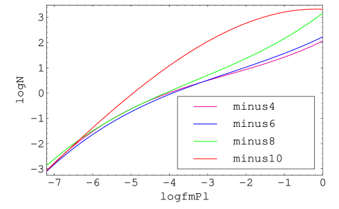
Figure 3: Number of $e$-folds depending on $\Lambda$ and $f$, with $\theta=\pi/100$.

One interesting thing is that locked inflationary phase [7] hardly occurs. This could be seen from the fact that there is no interaction term in the potential, e.g., such as $\lambda\phi^{2}\psi^{2}$. Thus the oscillation of, say, $\phi$ is not transmitted to the effective mass of $\psi$ to hold the field at a saddle point. Note that even if we include an interaction term of the form

$$\frac{\Lambda_{\phi}^{4}\Lambda_{\psi}^{4}}{m_{\mathrm{Pl}}^{4}}\cos\left(\frac{2\pi\phi}{f_{\phi}}\right)\cos\left(\frac{2\pi\psi}{f_{\psi}}\right)\,,$$ (9)

this term is suppressed by $m_{\mathrm{Pl}}^{4}$ and does not lead to any significant change. Also we note that the dependence of the number of $e$-folds on the initial misalignment $\theta$ [8] is very weak. We are considering $f\lesssim m_{\mathrm{Pl}}$, and the slow-roll parameter $|\eta|\gtrsim\mathcal{O}(1)$, see Eq. (3). Hence the field is very quickly rolling, and this makes the total number of $e$-folds more or less the same irrespective of the initial misalignment $\theta$. In Table 1, we present several results depending on $\theta$.

$\theta$	$\pi/100$	$\pi/40$	$\pi/20$	$\pi/10$	$\pi/8$	$\pi/5$
$N$	30.4465	30.2241	30.2100	30.1144	30.3783	30.0687

Table 1: Several results depending on different initial misalignment $\theta$. Parameters are given by $\Lambda=10^{-10}m_{\mathrm{Pl}}$ and $f=m_{\mathrm{Pl}}$. Note that the number of $e$-folds varies less than 1.

Now let us turn our attention to the perturbations produced during inflation. At the early stage of inflation when the field is very close to a maximum, we can split the field into the radial and angular components $\varphi$ and $\theta$, i.e.

$$\varphi=\sqrt{\phi^{2}+\psi^{2}}\,,$$ (10)

and $\theta$ as Eq. (5). Note that near a maximum, $U(1)$ symmetry is good enough. The radial component $\varphi$ thus plays the role of the “inflaton”, yielding adiabatic perturbations, while the angular component $\theta$ is orthogonal to the field trajectory and its fluctuations correspond to the isocurvature perturbations. Therefore the radial fluctuations follow the form of those from the usual inverted quadratic potential [10], but the angular ones are very close to those of massless scalar field and the spectrum is nearly scale invariant [8, 11]. Now, we can follow the $\delta N$ formalism [9] to write the power spectrum of the primordial density perturbations as

$$\mathcal{P} =\sum_{i}\left(\frac{\partial N}{\partial\phi_{i}}\right)^{2}\mathcal{P}_{\phi_{i}}$$

$$=\left(\frac{\partial N}{\partial\varphi}\right)^{2}\mathcal{P}_{\varphi}+\left(\frac{\partial N}{\partial\theta}\right)^{2}\mathcal{P}_{\theta}\,,$$ (11)

where it is clear that both the adiabatic and the isocurvature components contribute to the final perturbations. For the isocurvature perturbations to dominate the primordial perturbations, we require that

$$\left(\frac{\partial N}{\partial\theta}\right)^{2}\gg\left(\frac{\partial N}{\partial\varphi}\right)^{2}\,.$$ (12)

Since the adiabatic component is boosted by a factor of $1/\sqrt{\epsilon}$, generally we need $\left(\partial N/\partial\theta\right)^{2}\gg 1$, i.e., the number of $e$-folds is highly dependent on where the field is rolling towards. But as we have seen in Table 1, the number of $e$-folds is more or less the same irrespective of the misalignment. Thus $(\partial N/\partial\theta)^{2}\ll 1$ so the contribution of the isocurvature component is negligible, and the density perturbation spectrum is completely dominated by the contribution of the inflaton component which is highly scale dependent.

Now let us consider the case when $f_{\phi}\neq f_{\psi}$, i.e. the potential is not symmetric but “squeezed”. Then, the field tends to roll along the squeezed direction first irrespective of the initial misalignment, because that direction is (much) steeper than the other one. Hence the isocurvature perturbations, i.e. the perturbations orthogonal to the field trajectory, become irrelevant and the “inflaton” perturbations are dominant. Let us assume that $\psi$ direction is squeezed so that $f_{\phi}=\alpha f_{\psi}$ with $\alpha>1$. With the rotated slow-roll parameters

$$\eta_{\sigma\sigma} =\eta_{\phi\phi}\cos^{2}\theta+\eta_{\psi\psi}\sin^{2}\theta\,$$

$$\eta_{ss} =\eta_{\phi\phi}\sin^{2}\theta+\eta_{\psi\psi}\cos^{2}\theta\,,$$ (13)

where $\sigma$ and $s$ denote the inflaton and the isocurvature components respectively, the evolution of the isocurvature perturbations is given by [12]

$$\dot{\mathcal{S}} \simeq(-2\epsilon+\eta_{\sigma\sigma}-\eta_{ss})H\mathcal{S}$$

$$=\left[-2\epsilon+\frac{\alpha^{2}-1}{\alpha^{2}}\frac{m_{\mathrm{Pl}}^{2}}{f_{\psi}^{2}}\left(\cos^{2}\theta-\sin^{2}\theta\right)\right]H\mathcal{S}$$

$$\simeq\left(-2\epsilon-\frac{\alpha^{2}-1}{\alpha^{2}}\frac{m_{\mathrm{Pl}}^{2}}{f_{\psi}^{2}}\right)H\mathcal{S}\,,$$ (14)

which is always negative. Intuitively, as a direction becomes more and more squeezed, the potential becomes closer to the single field case where only the inflaton perturbations exist.

4 Remedies

In the previous section, we have seen that the number of $e$-folds obtained during inflation driven by two decoupled string axion fields is generally not enough to solve many cosmological problems. Also the power spectrum of density perturbations is completely dominated by the radial contribution which is not scale invariant. The naive inflation model of the two string axions is thus not sufficient and we need some amendments to improve the situation. In this section we briefly summarise some known remedies.

One obvious modification is to add more contribution to $H$ so that the field receives greater friction and can roll down the potential slowly. One would be tempted to add a positive cosmological constant, but this may cause two difficulties. When the cosmological constant is too large, it may render the universe to expand forever even after the field has settled down at a minimum. Also, since the observed dark energy density is of $\mathcal{O}\left(10^{-12}\mathrm{eV}^{4}\right)$, the magnitude of the cosmological constant one would like to add is severely constrained. It is possible, however, to increase $H$ by adding more fields and make them rolling slowly for many $e$-folds [13]. Then Eq. (4) becomes

$$\phi_{i}^{\prime\prime}+3\phi_{i}^{\prime}-\frac{\sum_{j}{\phi_{j}^{\prime}}^{2}}{2m_{\mathrm{Pl}}^{2}}\phi_{i}^{\prime}+\frac{V_{,i}\left(6m_{\mathrm{Pl}}^{2}-\sum_{j}{\phi_{j}^{\prime}}^{2}\right)}{2\left(V+3m_{\mathrm{Pl}}^{2}H_{0}^{2}\right)}=0\,,$$ (15)

where the contribution $H_{0}$ by other fields is dependent on models: for example, if we adopt N-flation [14] and add $k$ additional axions, we have

$$3m_{\mathrm{Pl}}^{2}H_{0}^{2} =V$$

$$\simeq\sum_{k}\frac{1}{2}m_{k}^{2}\phi_{k}^{2}\,,$$ (16)

where we assume that each axion field is displaced not too far from the minimum. It is possible that by some of the added fields further perturbations are generated after inflation [16], but the parameter space is heavily restricted for this mechanism to work properly [17].

Another clear way we can take is to make the axion decay constant $f$ larger than $m_{\mathrm{Pl}}$ and follow the original wisdom of natural inflation [18]. One difficulty we meet is that because it is required that $f\gg m_{\mathrm{Pl}}$ to satisfy the slow-roll conditions, $f$ is outside the region of the effective field theory description and is out of our control. An interesting alternative to build a model where the above problem could be evaded is to identify the extra component $A_{5}$ of a gauge field in a 5D theory with the inflaton [19]. Because this model is based on higher dimensional theory, the effective decay constant $f_{\mathrm{eff}}=(2\pi g_{4D}R)^{-1}\gg m_{\mathrm{Pl}}$, where $R$ is the radius of the circle where the extra dimension is compactified, is reliable. Another way of constructing $f>m_{\mathrm{Pl}}$ is to incorporate two different gauge groups, making the effective decay constant larger than $m_{\mathrm{Pl}}$ by imposing a symmetric relation between the couplings of the axions to the gauge groups [20]. In Fig. 4 several results of $e$-folds depending on $f$ and $\theta$ are shown. Note that when the field rolls towards a saddle point, generally it acquires extra $e$-folds but the scale invariance of the perturbation spectrum is broken when the field leaves the saddle point [21]. To avoid this, we should put strong constraints on the parameters [6].

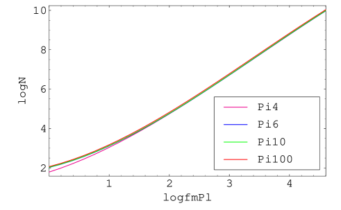
Figure 4: Plot of $N$ versus $f$ and $\theta$. The energy scale $\Lambda$ is set to be $10^{-4}m_{\mathrm{Pl}}$. We can see that as $f$ becomes bigger, we obtain larger $N$ as expected. Also note that the dependence on $\theta$ is not significant.

Also note that when $f\gg m_{\mathrm{Pl}}$, the minima are separated by a distance far larger than $m_{\mathrm{Pl}}$. Hence, the extrema which intervene between those minima become the sources of eternal topological inflation [22]. For example, a saddle point which separates two minima along (say) $\psi$ direction, it becomes a domain wall and in its vicinity we have an eternally inflating regime.

One fundamental question we can ask at this point is whether it is possible to find regimes of moduli space where $f\gg m_{\mathrm{Pl}}$ in string theory. It seems that, unfortunately, there exists no consistent scenario yet [23] although not all the possibilities are explored. Building a consistent scenario where a large decay constant could arise is still an interesting and challenging topic.

5 Summary

We have investigated a simple inflation model which consists of two non-interacting axions. The number of $e$-folds $N$ achieved while the field rolls off from a maximum is dependent on both the energy scale $\Lambda$ and the decay constant $f$: we obtain larger $N$ with smaller $\Lambda$ and with bigger $f$, but generally $N$ is not sufficient to solve cosmological problems. Interestingly, in spite of the rich geometry of the potential, the initial misalignment $\theta$ hardly affects $N$ because of the absence of the interaction term, which also leads to no locked inflationary phase. The perturbation spectrum is highly scale dependent, because the scale invariant spectrum which arises from the isocurvature component is greatly suppressed. To alleviate this situation, we may either increase $H$ by adding more axion fields, or make $f$ bigger than $m_{\mathrm{Pl}}$ which is still unclear in the context of string theory.

Acknowledgements

I am grateful to James Cline and Richard Easther for helpful comments. It is a great pleasure to thank Alexei Starobinsky for invaluable correspondences on the adiabatic and isocurvature perturbations. I also thank the organisers of the 86th Les Houches Summer Session where some part of this work was carried out.

References

- [1] See, e.g. A. R. Liddle and D. H. Lyth, Cosmological inflation and large scale structure, Cambridge University Press (2000)
- [2] S. Kachru, R. Kallosh, A. Linde and S. P. Trivedi, Phys. Rev. D 68, 046005 (2003) hep-th/0301240
- [3] See, e.g. A. Linde, hep-th/0503195
- [4] J. E. Kim, Phys. Rept. 150, 1 (1987) ; M. Y. Khlopov and S. G. Rubin, Cosmological Pattern Of Microphysics In The Inflationary Universe, Kluwer Academic Publishers (2004)
- [5] See, e.g. D. H. Lyth and A. Riotto, Phys. Rept. 314, 1 (1999) hep-ph/9807278
- [6] R. Easther, J. Khoury and K. Schalm, J. Cosmol. Astropart. Phys. 06, 006 (2004) hep-th/0402218
- [7] G. Dvali and S. Kachru, hep-th/0309095
- [8] K. Kadota and E. D. Stewart, J. High Energy Phys. 12, 008 (2003) hep-ph/0311240
- [9] A. A. Starobinsky, JETP Lett. 42, 152 (1985) ; M. Sasaki and E. D. Stewart, Prog. Theor. Phys. 95, 71 (1996) astro-ph/9507001 ; M. Sasaki and T. Tanaka, Prog. Theor. Phys. 99, 763 (1998) gr-qc/9801017 ; J.-O. Gong and E. D. Stewart, Phys. Lett. B 538, 213 (2002) astro-ph/0202098
- [10] E. D. Stewart and J.-O. Gong, Phys. Lett. B 510, 1 (2001) astro-ph/0101225
- [11] C. T. Byrnes and D. Wands, Phys. Rev. D 73, 063509 (2006) astro-ph/0512195
- [12] D. Wands, N. Bartolo, S. Matarrese and A. Riotto, Phys. Rev. D 66, 043520 (2002) astro-ph/0205253
- [13] A. R. Liddle, A. Mazumdar and F. E. Schunck, Phys. Rev. D58, 061301 (1998) astro-ph/9804177 ; P. Kanti and K. Olive, Phys. Rev. D 60, 043502 (1999) hep-ph/9903524 ; E. J. Copeland, A. Mazumdar and N. J. Nunes, Phys. Rev. D 60, 083506 (1999) astro-ph/9904309
- [14] S. Dimopoulos, S. Kachru, J. McGreevy and J. G. Wacker, hep-th/0507205
- [15] J.-O. Gong, hep-th/0611293
- [16] D. H. Lyth and D. Wands, Phys. Lett. B 524, 5 (2002) hep-ph/0110002 ; T. Moroi and T. Takahashi, Phys. Lett. B 522, 215 (2002) hep-ph/0110096 Erratum-ibid. B 539, 303 (2002)
- [17] J.-O. Gong, Phys. Lett. B 637, 149 (2006) hep-ph/0602106
- [18] K. Freese, J. A. Frieman and A. V. Olinto, Phys. Rev. Lett. 65, 3233 (1990) ; F. C. Adams, J. R. Bond, K. Freese, J. A. Frieman and A. V. Olinto, Phys. Rev. D 47, 426 (1993) hep-ph/9207245
- [19] N. Arkani-Hamed, H.-C. Cheng, P. Ceminelli and L. Randall, Phys. Rev. Lett. 90, 221302 (2003) hep-th/0301218
- [20] J. E. Kim, H. P. Nilles and M. Peloso, J. Cosmol. Astropart. Phys. 01, 005 (2005) hep-ph/0409138
- [21] J. Choe, J.-O. Gong and E. D. Stewart, J. Cosmol. Astropart. Phys. 07, 012 (2004) hep-ph/0405155 ; M. Joy, E. D. Stewart, J.-O. Gong and H.-C. Lee, J. Cosmol. Astropart. Phys. 04, 012 (2005) astro-ph/0501659 ; J.-O. Gong, J. Cosmol. Astropart. Phys. 07, 015 (2005) astro-ph/0504383 ; J.-O. Gong, AIP Conf. Proc. 805, 451 (2006)
- [22] A. Vilenkin, Phys. Rev. Lett. 72, 3137 (1994) hep-th/9402085 ; A. D. Linde and D. A. Linde, Phys. Rev. D 50, 2456 (1994) hep-th/9402115
- [23] T. Banks, M. Dine, P. J. Fox and E. Gorbatov, J. Cosmol. Astropart. Phys. 06, 001 (2003) hep-th/0303252