Initial Singularity of the Little Bang

Abstract

The Color Glass Condensate (CGC) predicts the form of the nuclear wavefunction in QCD at very small $x$. Using this, we compute the wavefunction for the collision of two nuclei, infinitesimally in the forward light cone. We show that the Wigner transformation of this wavefunction generates rapidity dependent fluctuations around the boost invariant classical solution which describe the Glasma in the forward light cone.

1. RIKEN BNL Research Center,
   Brookhaven National Laboratory,
   Upton, NY-11973, USA

2. Service de Physique Théorique (URA 2306 du CNRS)
   CEA/DSM/Saclay, Bât. 774
   91191, Gif-sur-Yvette Cedex, France

3. Department of Physics, Bldg. 510 A,
   Brookhaven National Laboratory,
   Upton, NY-11973, USA

1 Introduction

The Color Glass Condensate (CGC) provides a description of the wavefunction of a hadron at very small values of $x$ [1, 2, 3, 4, 5]. The CGC is a high density state of gluons which is controlled by a weak coupling, due to the high gluon density. Its properties are computable from first principles in QCD, at least in the limit of extremely high density.

The CGC has also been applied to heavy ion collisions in order to generate the initial conditions for the evolution of matter in the forward light cone [6, 7, 8, 9, 10]. There are boost invariant solutions of the equations of motion supposedly appropriate for the high energy limit. The matter in the forward light cone, which we call the Glasma [10], initially has large longitudinal color electric and magnetic fields, and as well as a large value of the Chern-Simons charge density. As time evolves, transverse color electric and magnetic fields appear as the remnants of the decaying longitudinal fields. This occurs as a consequence of the classical equations of motion. Eventually as the system becomes very dilute, these transverse color electric and magnetic fields may be treated as gluons, which form a quark-gluon plasma. The solution to the classical equations of motion is boost invariant and describes a system of expanding classical fields.

It has recently been discovered that the boost invariant solution of the equations of motion are unstable with respect to rapidity dependent perturbations [11]. This instability has in fact close connections with the Weibel instabilities encountered in the physics of anisotropic plasmas [12, 13, 14], and it is speculated that such an instability may help the system created after heavy ion collisions reach a state of local equilibrium [15, 16, 17, 18, 19, 20, 21]. Whether or not such instabilities can grow to sufficient magnitude as to become as large as the classical solution is the subject of current investigations. One piece of the puzzle which is not yet understood is the spectrum of the initial fluctuations. It is the purpose of this paper to derive an expression for the probability distribution of these fluctuations.

If such fluctuations can grow to a magnitude comparable to the classical boost invariant field, then one has amplified initial quantum fluctuations to macroscopic chaotic turbulence. Such turbulence may ultimately be responsible for producing a thermalized Quark Gluon Plasma. Indeed, it proves difficult to thermalize an expanding system of quarks and gluons by conventional multiple scattering formulae [22].

The evolution from the initial collision to the final state is shown in Fig. 1. Because of the similarities between the expansion of the universe in cosmology and the expansion of matter in heavy ion collisions, we call the latter the “little bang”. The initial singularity of cosmology is replaced by the singularity in the classical equations of motion associated with the collision. As in cosmology, where topological transitions associated with Chern-Simons charge may be responsible for generating baryon number, during the Glasma phase, there are also topological helicity flip transitions [10, 23]. It is during this time that instabilities develop, and there may be a Kolmogorov spectrum of density fluctuations generated [16, 19, 24]. This spectrum is similar to the spectrum of density fluctuations generated during inflationary cosmology. After inflation, the system reheats and thermalizes forming an electroweak plasma. In the little bang, thermalization might also be achieved after the Glasma expansion. Of course such an analogy between the little bang is not perfect, and it has not been established that the Glasma can in fact become thermalized. Nevertheless, in the little bang, all of the physics is in principle understood from QCD in a small coupling regime, and one should be able ultimately to compute the evolution of the system.

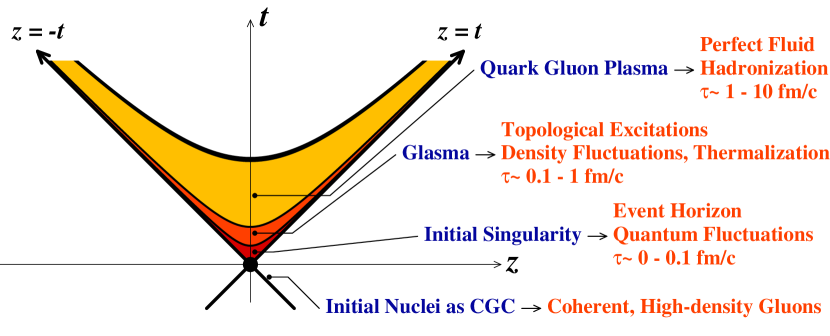
Figure 1: A light cone diagram illustrating the evolution of matter produced in heavy ion collisions

We begin this paper by a discussion of the evolution of an unstable system in quantum mechanics. We discuss a Gaussian initial wavefunction in the path-integral representation in which a description equivalent to the Schwinger-Keldysh formalism [25] naturally arises. We show that the distribution of initial fluctuations is given by the Wigner transform of the quantum mechanical wavefunction [26]. These initial fluctuations are further evolved by solving classical equations of motion. We then proceed to show that the same procedure works in quantum field theory. We then compute the quantum field theoretical wavefunction which describes the collision of two hadrons, at a time infinitesimally in the forward light-cone, after the collision. This should provide a practical algorithm for the computation of the evolution of matter produced in very high energy heavy ion collisions.

The necessity of summing over the initial quantum fluctuations when solving the classical Yang-Mills equations also appears when one goes beyond the classical approximation for the description of the fields in the forward light-cone. The formalism necessary for calculating loop corrections in a regime of strong sources and fields has been developed in Ref. [27] (and applied to the computation of the production of quark pairs – the simplest among the NLO contributions – in Ref. [28]). In this systematic approach, the instability of the boost invariant classical solution manifests itself as a divergence in the one-loop correction to the inclusive gluon spectrum, and it seems that the resummation of these divergent terms leads directly to an average over fluctuations of the classical initial conditions [29].

The description we advocate here has also some philosophical similarities with the work of Kharzeev et al., who make an analogy to Hawking radiation [30]. We are unable to identify a Hawking temperature in our computation, but the idea that there is an initial spectrum of fluctuations generated at the initial singularity due to a quantum treatment of this singularity is similar.

2 The Case of Quantum Mechanics

2.1 General Formulation

We shall consider the time evolution of a generic quantum mechanical system from the initial time $t_{{}_{I}}$ to the final time $t_{{}_{F}}$. If the system is as simple as an harmonic oscillator, the quantum fluctuations at the final time $t_{{}_{F}}$ can be expressed in terms of the initial quantum fluctuation at $t_{{}_{I}}$ which evolve according to the classical equations of motion. In more complicated situations beyond the harmonic oscillator problem, the formulation we develop in what follows still holds unchanged, as long as we can make a Gaussian approximation in the weak coupling regime.

Let us consider a simple example [31]. Supposing that we have a convex parabolic potential as sketched in Fig. 2 until the initial time $t_{{}_{I}}$, we know that the ground state has a Gaussian distribution of quantum fluctuations around the minimum of the potential. Let us now assume that the potential suddenly becomes inverted at $t_{{}_{I}}$ : then the system is subject to an instability. If the problem was purely classical, the unstable state would not decay at all provided it lies exactly on the top of the potential curve. The decay into stable states is however unavoidable in quantum mechanics because of quantum fluctuations around the minimum. As long as higher order quantum fluctuations are negligible, it should be acceptable to approximate the time evolution classically under such a potential causing the instability. As a result, we can anticipate that the convolution of the initial dispersion and the classical evolution provides the later distribution of quantum fluctuations at $t_{{}_{F}}$, and we shall verify this in the forthcoming discussion. We would like to emphasize here that our formulation is not limited to this sort of specific instability problem, but applicable to more generic problems.

Figure 2: Schematic picture of the time evolution of quantum fluctuations. The ground state of a steady system for $t<t_{{}_{I}}$ has a Gaussian distribution of quantum fluctuations. The distribution at a later time $t_{{}_{F}}$ is given by the classical evolution from the initial distribution at $t=t_{{}_{I}}$.

In the language of quantum physics the ground state wavefunction at $t_{{}_{I}}$ embodies the zero-point oscillation. The position and momentum fluctuate according to the uncertainty principle. The expectation value of physical observables is defined as an average weighted by the wavefunction. Let us consider an observable $\mathcal{O}(x_{{}_{F}})$ which is a function of the position $x_{{}_{F}}$ at the final time $t_{{}_{F}}$. [We specifically denote the position variable at $t_{{}_{I}}$ and $t_{{}_{F}}$ as $x_{{}_{I}}$ and $x_{{}_{F}}$ respectively in order to distinguish them from the position at other times.] By definition the expectation value at $t_{{}_{F}}$ is given by

$$\langle\mathcal{O}\rangle_{t_{{}_{F}}}=\int\mathrm{d}x_{{}_{F}}\,\left|\psi(x_{{}_{F}},t_{{}_{F}})\right|^{2}\,\mathcal{O}(x_{{}_{F}})\;.$$ (1)

One can easily generalize the above expression to a situation involving observables that depend not only on the position $x_{{}_{F}}$ but also on the momentum $p_{{}_{F}}$. Using $p_{{}_{F}}=-\mathrm{i}\partial/\partial x_{{}_{F}}$ and $\mathcal{O}(x_{{}_{F}},-\mathrm{i}\partial/\partial x_{{}_{F}})$ acting on $\psi(x_{{}_{F}},t_{{}_{F}})$, one can reach the same conclusion as in Eq. (10) in what follows, but for simplicity we only perform the derivation for the case of Eq. (1).

The path-integral formulation naturally provides us the relation between the initial and final wavefunctions,

$$\psi(x_{{}_{F}},t_{{}_{F}})=\int\mathrm{d}x_{{}_{I}}\,\big{[}\mathcal{D}x(t)\,\mathcal{D}p(t)\big{]}\,\psi(x_{{}_{I}},t_{{}_{I}})\,\exp\biggl{\{}\,\mathrm{i}\int_{t_{{}_{I}}}^{t_{{}_{F}}}\!\mathrm{d}t\,\bigl{[}p\dot{x}-H(p,x)\bigr{]}\biggr{\}}\;,$$ (2)

where the integrals over the paths $x(t)$ and $p(t)$ extend from $t_{{}_{I}}$ to $t_{{}_{F}}$, with the boundary condition $x(t_{{}_{I}})=x_{{}_{I}}$ and $x(t_{{}_{F}})=x_{{}_{F}}$. The Hamiltonian is denoted by $H(p,x)$. We will perform the path-integral approximately in order to find an analytically manageable expression.

We expand the phase in the exponential around the stationary point, in order to reduce Eq. (2) to Gaussian functional integrals. The stationary condition leads to the classical path $x=x^{\text{c}}(t)$ and $p=p^{\text{c}}(t)$ determined by Hamilton’s equations of motion,

$$\dot{x^{\text{c}}}=\frac{\partial H(p^{\text{c}},x^{\text{c}})}{\partial p^{\text{c}}},\qquad\dot{p^{\text{c}}}=-\frac{\partial H(p^{\text{c}},x^{\text{c}})}{\partial x^{\text{c}}}$$ (3)

with the initial conditions $x^{\text{c}}(t_{{}_{I}})=x_{{}_{I}}$ and $p^{\text{c}}(t_{{}_{I}})=p_{{}_{I}}$. We note that the final position $x^{\text{c}}_{{}_{F}}(x_{{}_{I}},p_{{}_{I}})\equiv x^{\text{c}}(t_{{}_{F}})$ is unique with $x_{{}_{I}}$ and $p_{{}_{I}}$ given, which means that we must consider the initial momentum $p_{{}_{I}}$ as a function of $x_{{}_{I}}$ and $x_{{}_{F}}$. Naturally, the quantum fluctuation around the classical path must be restricted at $t_{{}_{I}}$ and $t_{{}_{F}}$ to satisfy the boundary condition $\delta x(t_{{}_{I}})=\delta x(t_{{}_{F}})=0$. Up to the quadratic order in quantum fluctuations, therefore, we have

$$\begin{split}&\psi(x_{{}_{F}},t_{{}_{F}})=\int\mathrm{d}x_{{}_{I}}\,\psi(x_{{}_{I}},t_{{}_{I}})\,\exp\biggl{\{}\,\mathrm{i}\int_{t_{{}_{I}}}^{t_{{}_{F}}}\!\mathrm{d}t\bigl{[}p^{\text{c}}\dot{x^{\text{c}}}-H(p^{\text{c}},x^{\text{c}})\bigr{]}\biggr{\}}\\ &\qquad\qquad\times\!\!\!\!\int\limits_{\delta x(t_{{}_{I}})=\delta x(t_{{}_{F}})=0}\!\!\!\!\!\!\!\!\!\!\!\!\big{[}\mathcal{D}\delta x(t)\,\mathcal{D}\delta p(t)\big{]}\,\exp\biggl{\{}\,\mathrm{i}\int_{t_{{}_{I}}}^{t_{{}_{F}}}\!\mathrm{d}t\Bigl{[}\delta p\,\delta\dot{x}\\ &\qquad\qquad\qquad\qquad\qquad-\frac{\partial^{2}H}{\partial p^{2}}\delta p^{2}\!-\!\frac{\partial^{2}H}{\partial x^{2}}\delta x^{2}\!-\!2\frac{\partial^{2}H}{\partial p\,\partial x}\delta p\,\delta x\Bigr{]}\biggr{\}}\;.\end{split}$$ (4)

In the expansion of the argument of the exponential, the linear order terms in the fluctuations vanish because of the classical equations of motion. The first integral in the above expression is the classical part corresponding to the WKB approximation, where the $x_{{}_{F}}$ dependence is implicit through the fact that $x^{\text{c}}(t)$ is the classical trajectory that starts at $x_{{}_{I}}$ and ends at $x_{{}_{F}}$. The second integral represents the one-loop quantum corrections leading to the determinant of the propagator with the Dirichlet boundary condition. It is obvious from the above expression that, if $H$ is the Hamiltonian of an harmonic oscillator (therefore consisting only of quadratic terms in $x$ and $p$), e.g., $H=\textstyle\frac{1}{2}p^{2}+\textstyle\frac{1}{2}\omega^{2}x^{2}$, the WKB approximation is exact. It is because none of $\partial^{2}H/\partial p^{2}\!=\!1$, $\partial^{2}H/\partial x^{2}\!=\!\omega^{2}$, and $\partial^{2}H/\partial p\,\partial x\!=\!0$ depends on $x_{{}_{I}}$ nor $p_{{}_{I}}$, and thus the integration with respect to fluctuations merely produces an irrelevant purely numerical factor.

In general, the one-loop integral gives $[\det G^{-1}(x^{\text{c}})]^{-1/2}$ where $G$ is the propagator of a fluctuation in the presence of the classical background $x^{\text{c}}$. Usually, this determinant has no explicit $p^{\text{c}}$ dependence since usual quantum theories have at most quadratic terms with respect to the canonical momenta. These quantum corrections alter $H(p^{\text{c}},x^{\text{c}})$ to be $H(p^{\text{c}},x^{\text{c}})-\frac{\mathrm{i}}{2}\ln G^{-1}(x^{\text{c}})$ and can be seen as an effective potential in the classical Hamiltonian.

From now on we assume that the $x^{\text{c}}$ dependence in $H(p^{\text{c}},x^{\text{c}})$ is so strong that we can drop the $x^{\text{c}}$ dependence from the quantum corrections $-\frac{\mathrm{i}}{2}\ln G^{-1}(x^{\text{c}})$. This assumption should be checked case by case. Generally speaking, this is acceptable in instability problems like the one illustrated in Fig. 2. The quantum corrections modify the tree-level potential, which would eventually affect the equations of motion. But if the tree-level potential is steep enough, the alteration due to quantum corrections should be negligible. Hence, our treatment is equivalent to assuming that the time evolution is dominantly governed by the tree-level potential.

The probability distribution for the positions at final time is therefore calculated with the classical parts alone as

$$\begin{split}&\left|\psi(x_{{}_{F}},t_{{}_{F}})\right|^{2}=\int\mathrm{d}x_{{}_{I}}^{\prime}\,\mathrm{d}x_{{}_{I}}\,\psi^{\ast}(x_{{}_{I}}^{\prime},t_{{}_{I}}^{\prime})\psi(x_{{}_{I}},t_{{}_{I}})\\ &\qquad\qquad\times\exp\biggl{\{}\,\mathrm{i}\int_{t_{{}_{I}}}^{t_{{}_{F}}}\mathrm{d}t\,\Bigl{[}\bigl{(}p^{\text{c}}\dot{x^{\text{c}}}\!-\!H(p^{\text{c}},x^{\text{c}})\bigr{)}\!-\!\bigl{(}{p^{\text{c}}}^{\prime}\dot{x^{\text{c}}}^{\prime}\!-\!H({p^{\text{c}}}^{\prime},{x^{\text{c}}}^{\prime})\bigr{)}\Bigr{]}\biggr{\}}\;.\end{split}$$ (5)

The phase difference induced by the different initial conditions, $x_{{}_{I}}$ and $x_{{}_{I}}^{\prime}$, can be simplified thanks to Hamilton’s equations of motion (3) as

$$\int_{t_{{}_{I}}}^{t_{{}_{F}}}\mathrm{d}t\,\Bigl{[}\bigl{(}p^{\text{c}}\dot{x^{\text{c}}}\!-\!H(p^{\text{c}},x^{\text{c}})\bigr{)}\!-\!\bigl{(}{p^{\text{c}}}^{\prime}\dot{x^{\text{c}}}^{\prime}\!-\!H({p^{\text{c}}}^{\prime},{x^{\text{c}}}^{\prime})\bigr{)}\Bigr{]}$$

$$\qquad=\int_{t_{{}_{I}}}^{t_{{}_{F}}}\mathrm{d}t\int_{\{{p^{\text{c}}}^{\prime}(t),{x^{\text{c}}}^{\prime}(t)\}}^{\{p^{\text{c}}(t),x^{\text{c}}(t)\}}\biggl{\{}\mathrm{d}p^{\text{c}}\dot{x}+p^{\text{c}}\mathrm{d}\dot{x^{\text{c}}}-\frac{\partial H}{\partial p^{\text{c}}}\mathrm{d}p^{\text{c}}-\frac{\partial H}{\partial x^{\text{c}}}\mathrm{d}x^{\text{c}}\biggr{\}}$$

$$\qquad=-\int_{x_{{}_{I}}^{\prime}}^{x_{{}_{I}}}\mathrm{d}\tilde{x_{{}_{I}}}\;p_{{}_{I}}(\tilde{x_{{}_{I}}},x_{{}_{F}})\;.$$ (6)

From the middle to the last line only the surface term of the time integration remains. There is no finite contribution from the $t=t_{{}_{F}}$ side because $x_{{}_{F}}$ is common. It should be noted that $p_{{}_{I}}(x_{{}_{I}},x_{{}_{F}})$ in the last line is a function which gives the value of the initial momentum $p_{{}_{I}}$ as a function of the initial and final positions, i.e. $p_{{}_{I}}(x_{{}_{I}},x_{{}_{F}})=p_{{}_{I}}$ and $p_{{}_{I}}(x_{{}_{I}}^{\prime},x_{{}_{F}})=p_{{}_{I}}^{\prime}$. Here, in order to get a convenient expression, we shall define $P_{{}_{I}}$ as the initial momentum corresponding to the average of the two initial positions (and the same final position $x_{{}_{F}}$) by

$$P_{{}_{I}}\equiv p_{{}_{I}}(X_{{}_{I}},x_{{}_{F}})\;,$$ (7)

where $X_{{}_{I}}\equiv\textstyle\frac{1}{2}(x_{{}_{I}}+x_{{}_{I}}^{\prime})$. Then we can write the last line of Eq. (6) as follows,

$$-\int_{x_{{}_{I}}^{\prime}}^{x_{{}_{I}}}\mathrm{d}\tilde{x_{{}_{I}}}\;p_{{}_{I}}(\tilde{x_{{}_{I}}},x_{{}_{F}})= -\int_{-\textstyle\frac{1}{2}\delta x_{{}_{I}}}^{\textstyle\frac{1}{2}\delta x_{{}_{I}}}\mathrm{d}\Delta\tilde{x_{{}_{I}}}\;p_{{}_{I}}(X_{{}_{I}}+\Delta\tilde{x_{{}_{I}}},x_{{}_{F}})$$

$$\simeq -P_{{}_{I}}\delta x_{{}_{I}}-\frac{1}{24}\frac{\partial^{2}p_{{}_{I}}(X_{{}_{I}},x_{{}_{F}})}{\partial X_{{}_{I}}^{2}}\delta x_{{}_{I}}^{3}+\cdots$$ (8)

where we defined $\delta x_{{}_{I}}\equiv x_{{}_{I}}-x_{{}_{I}}^{\prime}$. Within the Gaussian approximation that we will employ later, it is enough for us to keep only the first term in the above expansion.

The expectation value at the final time is now transformed in the WKB approximation from Eq. (1) into

$$\langle\mathcal{O}\rangle_{t_{{}_{F}}}=\int\mathrm{d}x_{{}_{F}}\,\mathrm{d}x_{{}_{I}}^{\prime}\,\mathrm{d}x_{{}_{I}}\;\psi^{\ast}(x_{{}_{I}}^{\prime},t_{{}_{I}})\psi(x_{{}_{I}},t_{{}_{I}})\;\mathrm{e}^{-\mathrm{i}P_{{}_{I}}\delta x_{{}_{I}}}\,\mathcal{O}(x_{{}_{F}})\;.$$ (9)

Here we can replace the $x_{{}_{F}}$ integration by an integration over $P_{{}_{I}}$. Indeed, $x_{{}_{F}}$, $P_{{}_{I}}$ and $X_{{}_{I}}$ are related by the fact that the classical path that starts at the initial position $X_{{}_{I}}$ and with the initial momentum $P_{{}_{I}}$ ends at the position $x_{{}_{F}}$, i.e. $x_{{}_{F}}=x^{\text{c}}_{{}_{F}}(X_{{}_{I}},P_{{}_{I}})$. Such a replacement is accompanied by the Jacobian $|\partial x^{\text{c}}_{{}_{F}}/\partial P_{{}_{I}}|$ as a function of $X_{{}_{I}}$, $P_{{}_{I}}$, and $t_{{}_{F}}$. One can, in principle, obtain the Jacobian once one solves the classical path $x^{\text{c}}(x_{{}_{I}},p_{{}_{I}})$. This is, however, only a prefactor of the exponential for the phase of which we made the stationary-point approximation. It should be, therefore, consistent to drop the Jacobian prefactor off within the WKB approximation.

After all, rewriting $x_{{}_{I}}=X_{{}_{I}}+\textstyle\frac{1}{2}\delta x_{{}_{I}}$ and $x_{{}_{I}}^{\prime}=X_{{}_{I}}-\textstyle\frac{1}{2}\delta x_{{}_{I}}$ and integrating with respect to $\delta x_{{}_{I}}$, we formally reach the following expression,

$$\langle\mathcal{O}\rangle_{t_{{}_{F}}}$$

$$= \int\mathrm{d}X_{{}_{I}}\,\mathrm{d}\delta x_{{}_{I}}\,\mathrm{d}P_{{}_{I}}\,\psi^{\ast}(X_{{}_{I}}-\textstyle\frac{1}{2}\delta x_{{}_{I}},t_{{}_{I}})\psi(X_{{}_{I}}+\textstyle\frac{1}{2}\delta x_{{}_{I}},t_{{}_{I}})\,\mathrm{e}^{-\mathrm{i}P_{{}_{I}}\delta x_{{}_{I}}}\,\mathcal{O}\bigl{(}x^{\text{c}}_{{}_{F}}(X_{{}_{I}},P_{{}_{I}})\bigr{)}$$

$$= \int\mathrm{d}X_{{}_{I}}\,\mathrm{d}P_{{}_{I}}\;W(X_{{}_{I}},P_{{}_{I}})\;\mathcal{O}\bigl{(}x^{\text{c}}_{{}_{F}}(X_{{}_{I}},P_{{}_{I}})\bigr{)}\;,$$ (10)

where $W(X_{{}_{I}},P_{{}_{I}})$ is the Wigner transform of the product of the two initial wavefunctions, defined as

$$W(X_{{}_{I}},P_{{}_{I}})\equiv\int\mathrm{d}\delta x_{{}_{I}}\,\psi^{\ast}(X_{{}_{I}}-\textstyle\frac{1}{2}\delta x_{{}_{I}},t_{{}_{I}})\psi(X_{{}_{I}}+\textstyle\frac{1}{2}\delta x_{{}_{I}},t_{{}_{I}})\,\mathrm{e}^{-\mathrm{i}P_{{}_{I}}\delta x_{{}_{I}}}\;.$$ (11)

This is our formula and the purpose of our work is to calculate the Wigner function analytically for the problem of heavy ion collisions, which should be a necessary input for numerical studies provided that the classical equations of motion are solved.

2.2 Simple Example

It would be instructive to demonstrate how the formula (10) works for an harmonic oscillator for which explicit calculations are feasible. Let us estimate the average of the observable ${\mathcal{O}}\equiv x_{{}_{F}}^{2}$ in a direct computation and by means of Eq. (10) and then compare the results. As we have already mentioned, the WKB approximation is exact in the case of the harmonic oscillator problem, which means that the two results should coincide. This is a trivial check of the validity of our formula (10).

We shall characterize the initial state as a Gaussian [31];

$$\psi(x_{{}_{I}},t_{{}_{I}}=0)=\bigl{(}\pi^{\frac{1}{2}}b\bigr{)}^{-\frac{1}{2}}\exp\bigl{(}-x_{{}_{I}}^{2}/2b^{2}\bigr{)}\;.$$ (12)

The Green’s function in the inverted harmonic oscillator with the Hamiltonian $H=\textstyle\frac{1}{2}p^{2}-\textstyle\frac{1}{2}\omega^{2}x^{2}$, which is defined by

$$\bigl{(}\mathrm{i}\partial_{t}+\partial_{x}^{2}+\omega^{2}x^{2}\bigr{)}\,G(x,x^{\prime};t)=\delta(t)\delta(x-x^{\prime})\;,$$

$$\lim_{t\to 0^{+}}G(x,x^{\prime};t)=\delta(x-x^{\prime})\;,$$ (13)

is known [31] to be

$$G(x,x^{\prime};t)=\bigl{(}2\pi\mathrm{i}\sinh\omega t\bigr{)}^{-\frac{1}{2}}\exp\biggl{\{}\frac{\mathrm{i}}{2\sinh\omega t}\Bigl{[}(x^{2}+x^{\prime 2})\cosh\omega t-2xx^{\prime}\Bigr{]}\biggr{\}}\;,$$ (14)

from which we can directly calculate the wavefunctions at later time by

$$\psi(x_{{}_{F}},t_{{}_{F}})=\int\mathrm{d}x_{{}_{I}}\;G(x_{{}_{F}},x_{{}_{I}};t_{{}_{F}})\psi(x_{{}_{I}},0)\;.$$ (15)

What we are calculating is the expectation value of the position dispersion when the potential is inverted at the initial time $t_{{}_{I}}=0$. After some algebraic procedures we find,

$$\bigl{|}\psi(x_{{}_{F}},t_{{}_{F}})|^{2}=\bigl{[}\pi^{\frac{1}{2}}B^{2}(t_{{}_{F}})\bigr{]}^{-1}\exp\bigl{[}-x_{{}_{F}}^{2}/B^{2}(t_{{}_{F}})\bigr{]},$$ (16)

where $B^{2}(t_{{}_{F}})\equiv b^{2}\cosh^{2}\omega t_{{}_{F}}+b^{-2}\sinh^{2}\omega t_{{}_{F}}$. Then, it is straightforward to compute the average value of ${\mathcal{O}}=x_{{}_{F}}^{2}$,

$$\langle{\mathcal{O}}\rangle_{t_{{}_{F}}}=\int\mathrm{d}x_{{}_{F}}\,\bigl{|}\psi(x_{{}_{F}},t_{{}_{F}})\bigr{|}^{2}x_{{}_{F}}^{2}=\frac{1}{2}B^{2}(t_{{}_{F}})\;.$$ (17)

This result indicates that the dispersion of the position grows exponentially with increasing time under the inverted potential just as sketched in Fig. 2.

Let us next consider the same problem according to the formula (10). The Wigner function obtained from Eq. (12) is

$$W(X_{{}_{I}},P_{{}_{I}})=\frac{1}{\pi}\exp\bigl{(}-X_{{}_{I}}^{2}/b^{2}-b^{2}P_{{}_{I}}^{2}\bigr{)}\;,$$ (18)

where we have adjusted the normalization factor, though it is only an unimportant prefactor, so that $\int\mathrm{d}X_{{}_{I}}\,\mathrm{d}P_{{}_{I}}\,W(X_{{}_{I}},P_{{}_{I}})=1$. The classical path is fixed by Hamilton’s equations of motion with the initial inputs $x^{\text{c}}(0)=X_{{}_{I}}$ and $p^{\text{c}}(0)=P_{{}_{I}}$, leading to the final point at $t=t_{{}_{F}}$ as a function of $X_{{}_{I}}$ and $P_{{}_{I}}$,

$$x^{\text{c}}_{{}_{F}}(X_{{}_{I}},P_{{}_{I}})=X_{{}_{I}}\cosh\omega t_{{}_{F}}+\frac{P_{{}_{I}}}{\omega}\sinh\omega t_{{}_{F}}\;.$$ (19)

After performing Gaussian integrations we can readily arrive at the expectation value,

$$\langle\mathcal{O}\rangle_{t_{{}_{F}}}=\int\mathrm{d}X_{{}_{I}}\,\mathrm{d}P_{{}_{I}}\,W(X_{{}_{I}},P_{{}_{I}})\,{x^{\text{c}}_{{}_{F}}}^{2}(X_{{}_{I}},P_{{}_{I}})=\frac{1}{2}B^{2}(t_{{}_{F}})\;.$$ (20)

We see that our formula perfectly reproduces the result from the direct evaluation in this simple case of the harmonic oscillator. The merit of our method is that we do not have to calculate the Green’s function and the wavefunction at the final time directly.

3 Generalization to Quantum Field Theories

It is not difficult to extend the formula (10) described in Quantum Mechanics to the case of Quantum Field Theories. Let us consider in this section the case of a real scalar field theory.

3.1 Introduction

For a generic scalar field theory defined by a Hamiltonian density $\mathcal{H}[\phi,\pi]$ with field $\phi$ and canonical momentum $\pi$, we expect that the counterpart of Eq. (10) is

$$\langle\mathcal{O}\rangle_{t_{{}_{F}}}=\int\big{[}\mathrm{d}\phi_{{}_{I}}({\boldsymbol{x}})\big{]}\,\big{[}\mathrm{d}\pi_{{}_{I}}({\boldsymbol{x}})\big{]}\;W[\phi_{{}_{I}},\pi_{{}_{I}}]\;\mathcal{O}\big{[}\phi^{\text{c}}_{{}_{F}}[\phi_{{}_{I}},\pi_{{}_{I}}]\big{]}\;,$$ (21)

where $\phi^{\text{c}}_{{}_{F}}[\phi_{{}_{I}},\pi_{{}_{I}}]$ is the solution of the classical equations of motion at time $t_{{}_{F}}$ with the initial conditions $\phi^{\text{c}}(t_{{}_{I}},{\boldsymbol{x}})=\phi_{{}_{I}}({\boldsymbol{x}})$ and $\pi^{\text{c}}(t_{{}_{I}},{\boldsymbol{x}})=\pi_{{}_{I}}({\boldsymbol{x}})$. This classical field is a solution of Hamilton’s equations of motion,

$$\partial_{t}\phi^{\text{c}}=\frac{\delta H[\pi^{\text{c}},\phi^{\text{c}}]}{\delta\pi^{\text{c}}}\;,\qquad\partial_{t}\pi^{\text{c}}=-\frac{\delta H[\pi^{\text{c}},\phi^{\text{c}}]}{\delta\phi^{\text{c}}}\;.$$ (22)

Here $H$ denotes the integrated Hamiltonian $H\equiv\int\mathrm{d}^{3}{\boldsymbol{x}}\,\mathcal{H}$. The Wigner function is defined in the same way as in Quantum Mechanics by

$$W[\phi_{{}_{I}},\pi_{{}_{I}}]\equiv\int\big{[}\mathrm{d}\delta\phi_{{}_{I}}({\boldsymbol{x}})\big{]}\;\Psi^{\ast}[\phi_{{}_{I}}-\textstyle\frac{1}{2}\delta\phi_{{}_{I}},t_{{}_{I}}]\,\Psi[\phi_{{}_{I}}+\textstyle\frac{1}{2}\delta\phi_{{}_{I}},t_{{}_{I}}]\,\mathrm{e}^{-\mathrm{i}\int\!\mathrm{d}^{3}{\boldsymbol{x}}\,\pi_{{}_{I}}({\boldsymbol{x}})\delta\phi_{{}_{I}}({\boldsymbol{x}})}$$ (23)

in terms of the initial wavefunction $\Psi[\phi_{{}_{I}},t_{{}_{I}}]$. Similar expressions could be written for gauge fields after unphysical redundant degrees of freedom are removed by fixing the gauge. In the next subsection we will explain how one can construct the initial wavefunction $\Psi[\phi_{{}_{I}},t_{{}_{I}}]$ in practice.

3.2 Wavefunction from the Annihilation Operator

Let us consider the wavefunction and the associated Wigner function for the free real scalar field theory, which is the simplest extension to a Quantum Field Theory of the harmonic oscillator that we considered previously in Quantum Mechanics. In the Hamiltonian formulation, one can express the field operator $\hat{\phi}({\boldsymbol{x}})$ and its canonical momentum operator $\hat{\pi}({\boldsymbol{x}})$ in terms of the creation and annihilation operators as

$$\hat{\phi}({\boldsymbol{x}}) =\int\frac{\mathrm{d}^{3}{\boldsymbol{k}}}{(2\pi)^{3}}\frac{1}{\sqrt{2\omega_{k}}}\bigl{(}\hat{a}_{\boldsymbol{k}}\,\mathrm{e}^{\mathrm{i}{\boldsymbol{k}}\cdot{\boldsymbol{x}}}+\hat{a}_{\boldsymbol{k}}^{\dagger}\,\mathrm{e}^{-\mathrm{i}{\boldsymbol{k}}\cdot{\boldsymbol{x}}}\bigr{)}\;,$$ (24)

$$\hat{\pi}({\boldsymbol{x}}) =-\mathrm{i}\int\frac{\mathrm{d}^{3}{\boldsymbol{k}}}{(2\pi)^{3}}\sqrt{\frac{\omega_{k}}{2}}\bigl{(}\hat{a}_{\boldsymbol{k}}\,\mathrm{e}^{\mathrm{i}{\boldsymbol{k}}\cdot{\boldsymbol{x}}}-\hat{a}_{\boldsymbol{k}}^{\dagger}\,\mathrm{e}^{-\mathrm{i}{\boldsymbol{k}}\cdot{\boldsymbol{x}}}\bigr{)}\;,$$ (25)

in the Schroedinger representation in which operators are time independent. The dispersion relation for the free theory is $\omega_{k}=\sqrt{{\boldsymbol{k}}^{2}+m^{2}}$. The canonical quantization condition is $[\hat{\phi}({\boldsymbol{x}}),\hat{\pi}({\boldsymbol{x}}^{\prime})]=\mathrm{i}\delta^{(3)}({\boldsymbol{x}}-{\boldsymbol{x}}^{\prime})$ or equivalently $[\hat{a}_{\boldsymbol{k}},\hat{a}_{{\boldsymbol{k}}^{\prime}}^{\dagger}]=(2\pi)^{3}\delta^{(3)}({\boldsymbol{k}}-{\boldsymbol{k}}^{\prime})$. In momentum space, we have

$$\hat{\phi}({\boldsymbol{k}}) \equiv\int\mathrm{d}^{3}{\boldsymbol{x}}\;\hat{\phi}({\boldsymbol{x}})\;\mathrm{e}^{-\mathrm{i}{\boldsymbol{k}}\cdot{\boldsymbol{x}}}=\frac{1}{\sqrt{2\omega_{k}}}\bigl{(}\hat{a}_{\boldsymbol{k}}+\hat{a}_{-{\boldsymbol{k}}}^{\dagger}\bigr{)}\;,$$ (26)

$$\hat{\pi}({\boldsymbol{k}}) \equiv\int\mathrm{d}^{3}{\boldsymbol{x}}\;\hat{\pi}({\boldsymbol{x}})\;\mathrm{e}^{-\mathrm{i}{\boldsymbol{k}}\cdot{\boldsymbol{x}}}=-\mathrm{i}\sqrt{\frac{\omega_{k}}{2}}\bigl{(}\hat{a}_{\boldsymbol{k}}-\hat{a}_{-{\boldsymbol{k}}}^{\dagger}\bigr{)}\;,$$ (27)

for which the canonical commutation relation is deduced as $[\hat{\phi}({\boldsymbol{k}}),\hat{\pi}({\boldsymbol{k}}^{\prime})]=\mathrm{i}(2\pi)^{3}\delta^{(3)}({\boldsymbol{k}}-{\boldsymbol{k}}^{\prime})$. Let us consider an initial state which is an eigenstate of the operator $\hat{\phi}({\boldsymbol{k}})$,

$$\hat{\phi}({\boldsymbol{k}})\,\Psi[\phi_{{}_{I}},t_{{}_{I}}]=\phi_{{}_{I}}({\boldsymbol{k}})\;\Psi[\phi_{{}_{I}},t_{{}_{I}}]\;.$$ (28)

From the commutator between $\hat{\phi}({\boldsymbol{k}})$ and $\hat{\pi}({\boldsymbol{k}}^{\prime})$, we see that $\hat{\pi}({\boldsymbol{k}})$ can be represented as the differential operator with respect to the eigenvalue $\phi_{{}_{I}}(-{\boldsymbol{k}})$, that is,

$$\hat{\pi}({\boldsymbol{k}})\,\Psi[\phi_{{}_{I}},t_{{}_{I}}]=-\mathrm{i}\frac{\delta}{\delta\phi_{{}_{I}}(-{\boldsymbol{k}})}\,\Psi[\phi_{{}_{I}},t_{{}_{I}}]\;.$$ (29)

Here the functional derivative in momentum space is understood in our convention as $\delta f({\boldsymbol{k}})/\delta f({\boldsymbol{k}}^{\prime})=(2\pi)^{3}\delta^{(3)}({\boldsymbol{k}}-{\boldsymbol{k}}^{\prime})$. The ground state is the vacuum defined by the annihilation operator, i.e.

$$\hat{a}_{\boldsymbol{k}}\Psi[\phi_{{}_{I}},t_{{}_{I}}]=0\;.$$ (30)

Thus, the ground state should follow from

$$\hat{a}_{\boldsymbol{k}}\Psi[\phi_{{}_{I}},t_{{}_{I}}]=\frac{1}{2}\biggl{[}\sqrt{2\omega_{\boldsymbol{k}}}\,\phi_{{}_{I}}({\boldsymbol{k}})+\sqrt{\frac{2}{\omega_{k}}}\,\frac{\delta}{\delta\phi_{{}_{I}}(-{\boldsymbol{k}})}\biggr{]}\Psi[\phi_{{}_{I}},t_{{}_{I}}]=0\;.$$ (31)

It is easy to find the solution to the above equation being

$$\Psi[\phi_{{}_{I}},t_{{}_{I}}]\propto\biggl{(}\prod_{\boldsymbol{k}}\sqrt{\frac{\omega_{k}}{2\pi}}\biggr{)}\exp\biggl{[}-\int\frac{\mathrm{d}^{3}{\boldsymbol{k}}}{(2\pi)^{3}}\,\frac{\omega_{k}}{2}\,\phi_{{}_{I}}(-{\boldsymbol{k}})\phi_{{}_{I}}({\boldsymbol{k}})\biggr{]}.$$ (32)

The prefactor is the normalization for the Gaussian function, which is in fact unimportant in our approximation. The meaning of this wavefunction is that the ground state contains fluctuations with an energy $\omega_{k}/2$, that is, the zero-point energy. Then the Wigner function is

$$W[\phi_{{}_{I}},\pi_{{}_{I}}]=N\exp\biggl{[}-\int\frac{\mathrm{d}^{3}{\boldsymbol{k}}}{(2\pi)^{3}}\,\biggl{\{}\omega_{k}\,\phi_{{}_{I}}(-{\boldsymbol{k}})\phi_{{}_{I}}({\boldsymbol{k}})+\frac{1}{\omega_{k}}\,\pi_{{}_{I}}(-{\boldsymbol{k}})\pi_{{}_{I}}({\boldsymbol{k}})\biggr{\}}\biggr{]}$$ (33)

with a normalization prefactor $N$ independent of the fields and energy. One can clearly see that the result in the free real scalar field theory is just the product of the Wigner functions for an infinite assembly of independent harmonic oscillators (see Eq. (18)).

3.3 Wavefunction from the Schrödinger Equation

The strategy we used in the previous subsection, based on the canonical approach, is obvious but not very suitable for more complicated problems like those encountered in gauge theories. We will develop here an alternate method in order to find the ground state wavefunction.

In Quantum Mechanics, the wavefunction can usually be obtained as a solution of the Schrödinger equation when the Hamiltonian is provided. We will follow this procedure in the free real scalar field theory and will find a wavefunction that is exactly the same as what we have obtained in Eq. (32). Let us begin with the Lagrangian density defining the free real scalar field theory,

$$\mathcal{L}=\frac{1}{2}(\partial_{t}\phi)(\partial_{t}\phi)-\frac{1}{2}(\partial_{i}\phi)(\partial_{i}\phi)-\frac{1}{2}m^{2}\phi^{2}\;.$$ (34)

The canonical momentum is $\pi=\delta L/\delta(\partial_{t}\phi)=\partial_{t}\phi$ (where $L$ is the integrated Lagrangian $L\equiv\int\!\mathrm{d}^{3}{\boldsymbol{x}}\,\mathcal{L}$) and the Hamiltonian density is by definition,

$$\mathcal{H}\equiv\pi\dot{\phi}-\mathcal{L}=\frac{1}{2}\pi\pi+\frac{1}{2}(\partial_{i}\phi)(\partial_{i}\phi)+\frac{1}{2}m^{2}\phi^{2}\;.$$ (35)

Of course, we could have started directly with this Hamiltonian density, but using the Lagrangian density as our starting point is more appropriate when we work with more general system of coordinates. This is so because the canonical momentum varies according to the choice of the time variable and so does the Hamiltonian density.

From the equal-time commutation relation, $[\hat{\phi}(t,{\boldsymbol{x}}),\hat{\pi}(t,{\boldsymbol{x}}^{\prime})]=\mathrm{i}\delta^{(3)}({\boldsymbol{x}}-{\boldsymbol{x}}^{\prime})$, we see that the action of the momentum operator $\hat{\pi}({\boldsymbol{x}})$ on an eigenstate of $\hat{\phi}({\boldsymbol{x}})$ is identical to that of the derivative $-\mathrm{i}\delta/\delta\phi({\boldsymbol{x}})$. The Schrödinger equation, $\mathrm{i}\partial_{t}\Psi=H\Psi$, can be expressed as a functional differential equation by means of this identification. The time dependence is actually separable by an ansatz $\Psi=\mathrm{e}^{-\mathrm{i}Et}\Psi_{0}$ where $\Psi_{0}$ is $t$ independent. Then, the time independent Schrödinger equation arises as

$$\int\mathrm{d}^{3}{\boldsymbol{x}}\,\biggl{[}-\frac{1}{2}\frac{\delta^{2}}{\delta\phi({\boldsymbol{x}})^{2}}+\frac{1}{2}\phi({\boldsymbol{x}})\bigl{(}-\partial_{i}\partial_{i}+m^{2}\bigr{)}\phi({\boldsymbol{x}})\biggr{]}\Psi_{0}=E\Psi_{0}\;.$$ (36)

The ground state solution to this equation is a Gaussian,

$$\begin{split}\Psi_{0}[\phi_{{}_{I}}]=&N\exp\biggl{[}-\frac{1}{2}\int\mathrm{d}^{3}{\boldsymbol{x}}\,\phi_{{}_{I}}({\boldsymbol{x}})\sqrt{-\partial_{i}\partial_{i}+m^{2}}\phi_{{}_{I}}({\boldsymbol{x}})\biggr{]}\\ =&N\exp\biggl{[}-\int\frac{\mathrm{d}^{3}{\boldsymbol{k}}}{(2\pi)^{3}}\frac{\omega_{k}}{2}\phi_{{}_{I}}(-{\boldsymbol{k}})\phi_{{}_{I}}({\boldsymbol{k}})\biggr{]}\;,\end{split}$$ (37)

which is identical to the wavefunction (32). Note that the energy eigenvalue $E$ is given by

$$E=\int\mathrm{d}^{3}{\boldsymbol{x}}\int\frac{\mathrm{d}^{3}{\boldsymbol{k}}}{(2\pi)^{3}}\frac{\sqrt{k^{2}+m^{2}}}{2}\;,$$ (38)

which is nothing but the diverging zero-point energy. In principle, one could also write down the wavefunctions for excited states in terms of the Hermite polynomials.

3.4 Wavefunction in terms of the $\tau,\eta$ coordinates

For later convenience we shall see the same problem in the $\tau,\eta$ coordinates defined by

$$x^{0}+x^{3}=\tau\mathrm{e}^{\eta},\qquad x^{0}-x^{3}=\tau\mathrm{e}^{-\eta}\;.$$ (39)

These coordinates are a natural choice for the purpose of describing the space-time geometry of a collisions between two high energy projectiles. Commonly $\tau$ and $\eta$ are called the proper time and the rapidity respectively. The Lagrangian density in this coordinate system is

$$\tau\mathcal{L}=\frac{\tau}{2}(\partial_{\tau}\phi)(\partial_{\tau}\phi)-\frac{1}{2\tau}(\partial_{\eta}\phi)(\partial_{\eta}\phi)-\frac{\tau}{2}({\boldsymbol{\partial}}_{\perp}\phi)\cdot({\boldsymbol{\partial}}_{\perp}\phi)-\frac{\tau}{2}m^{2}\phi^{2}$$ (40)

including the measure $\sqrt{|g_{\mu\nu}|}=\tau$. From this Lagrangian, we see that the canonical momentum is given by $\pi=\tau\partial_{\tau}\phi$. Then the Hamiltonian density is

$$\tau\mathcal{H}=\frac{1}{2\tau}\pi\pi+\frac{\tau}{2}\biggl{[}\frac{1}{\tau^{2}}(\partial_{\eta}\phi)(\partial_{\eta}\phi)+({\boldsymbol{\partial}}_{\perp}\phi)\cdot({\boldsymbol{\partial}}_{\perp}\phi)+m^{2}\phi^{2}\biggr{]}\;.$$ (41)

Now that we have the Hamiltonian density, we can write down the time independent Schrödinger equation as follows,

$$\int\mathrm{d}\eta\,\mathrm{d}^{2}{\boldsymbol{x}}_{\perp}\biggl{\{}-\frac{1}{2\tau}\frac{\delta^{2}}{\delta\phi(\eta,{\boldsymbol{x}}_{\perp})^{2}}+\frac{\tau}{2}\phi(\eta,{\boldsymbol{x}}_{\perp})\Bigl{[}-\frac{\partial_{\eta}^{2}}{\tau^{2}}-{\boldsymbol{\partial}}_{\perp}^{2}+m^{2}\Bigr{]}\phi(\eta,{\boldsymbol{x}}_{\perp})\biggr{\}}\Psi_{0}=E\Psi_{0}\;.$$ (42)

The solution of the above Schrödinger equation is then

$$\begin{split}\Psi_{0}[\phi_{{}_{I}}]=&N\exp\biggl{[}-\frac{1}{2}\int\mathrm{d}\eta\,\mathrm{d}^{2}{\boldsymbol{x}}_{\perp}\,\phi_{{}_{I}}(\eta,{\boldsymbol{x}}_{\perp})\,\tau\sqrt{-(1/\tau^{2})\partial_{\eta}^{2}-{\boldsymbol{\partial}}_{\perp}^{2}+m^{2}}\,\phi_{{}_{I}}(\eta,{\boldsymbol{x}}_{\perp})\biggr{]}\\ =&N\exp\biggl{[}-\int\frac{\mathrm{d}k_{\eta}\,\mathrm{d}^{2}{\boldsymbol{k}}_{\perp}}{(2\pi)^{3}}\phi_{{}_{I}}(-{\boldsymbol{k}})\frac{\sqrt{(k_{\eta}/\tau)^{2}+{\boldsymbol{k}}_{\perp}^{2}+m^{2}}}{2\tau}\phi_{{}_{I}}({\boldsymbol{k}})\biggr{]}\;,\end{split}$$ (43)

where we defined the Fourier transform,

$$\phi({\boldsymbol{k}})\equiv\int\mathrm{d}\eta\,\mathrm{d}^{2}{\boldsymbol{x}}_{\perp}\,\tau\,\phi(\eta,x_{\perp})\,\mathrm{e}^{-\mathrm{i}(k_{\eta}\eta+{\boldsymbol{k}}_{\perp}\cdot{\boldsymbol{x}}_{\perp})}\;,$$ (44)

with ${\boldsymbol{k}}\equiv(k_{\eta},{\boldsymbol{k}}_{\perp})$. It is quite important to note that this wavefunction is $\tau$ independent because the seeming $\tau$ dependence is to be absorbed by the variable change $\eta\to\eta/\tau$ in the first line and $k_{\eta}\to\tau k_{\eta}$ in the second line. Of course, such rescaling changes the argument of the fields $\phi_{{}_{I}}(\eta,{\boldsymbol{x}}_{\perp})$ and $\phi_{{}_{I}}({\boldsymbol{k}})$ too. We will perform the integration over those fields at the end, however, and so the rescaling does not matter since possible $\tau$ dependence in $\phi_{{}_{I}}(\eta,{\boldsymbol{x}}_{\perp})$ and $\phi_{{}_{I}}({\boldsymbol{k}})$ would be absorbed in this integration. This feature is essential for our construction of the wavefunction, for we made use of the time independent Schrödinger equation with an ansatz $\Psi=\mathrm{e}^{-\mathrm{i}E\tau}\Psi_{0}$ where $\Psi_{0}$ is $\tau$ independent.

4 Non-Abelian Gauge Theory

We are now ready to proceed into the construction of the wavefunction in non-Abelian gauge theories. Before addressing the calculation of the wavefunction, we summarize our conventions, gauge choice, and basic equations. Then we will construct the wavefunction in the empty vacuum in the backward light cone region before the collision. We will connect the wavefunction from the infinitesimally backward light cone region to the infinitesimally forward light cone region with the boundary condition derived from the singularity in the Hamiltonian density.

4.1 Coordinates

Let us first recall our conventions for the light cone coordinates and for the $\tau,\eta$ coordinates. The light cone coordinates are defined by

$$x^{+}\equiv\frac{1}{\sqrt{2}}(t+z)\quad,\quad x^{-}\equiv\frac{1}{\sqrt{2}}(t-z)\;.$$ (45)

From there, we can readily obtain the metric tensor from the relation $\mathrm{d}s^{2}=g_{\mu\nu}\mathrm{d}x^{\mu}\mathrm{d}x^{\nu}$,

$$g_{+-}=g_{-+}=1\quad,\quad g_{xx}=g_{yy}=-1\;,$$ (46)

where the non-written components are all zero. Accordingly the light cone derivatives are to be understood as $\partial^{\pm}\equiv\partial/\partial x^{\mp}$.

The proper time $\tau$ and the rapidity variable $\eta$ have already been defined in Eq. (39), and are related to the light-cone coordinates by $x^{\pm}=(\tau/\sqrt{2})\mathrm{e}^{\pm\eta}$. The metric tensor for the $\tau,\eta$ coordinate system is diagonal, with

$$g_{\tau\tau}=1\quad,\quad g_{\eta\eta}=-\tau^{2}\quad,\quad g_{xx}=g_{yy}=-1\;.$$ (47)

Derivative with respect to $\tau,\eta$ and $x^{\pm}$ can be related thanks to the following relation,

$$\mathrm{d}x^{\pm}=\frac{x^{\pm}}{\tau}\mathrm{d}\tau\pm x^{\pm}\mathrm{d}\eta\;.$$ (48)

From the above identities, we can write the one-form gauge field as,

$$\begin{split}A_{\tau}\mathrm{d}\tau+A_{\eta}\mathrm{d}\eta&=A^{-}\mathrm{d}x^{+}+A^{+}\mathrm{d}x^{-}\\ &=\frac{1}{\tau}(x^{+}A^{-}+x^{-}A^{+})\mathrm{d}\tau+(x^{+}A^{-}-x^{-}A^{+})\mathrm{d}\eta\;.\end{split}$$ (49)

Therefore, the components of the gauge field in the $\tau,\eta$ coordinates are

$$A_{\tau}=A^{\tau}\equiv\frac{1}{\tau}(x^{+}A^{-}+x^{-}A^{+})\quad,\quad A_{\eta}=-\tau^{2}A^{\eta}\equiv x^{+}A^{-}-x^{-}A^{+}\;.$$ (50)

In the same way, we can obtain the field strength as the two-form $F=\mathrm{d}A-\mathrm{i}gA\wedge A$, that is,

$$F_{\tau\eta}\equiv\partial_{\tau}A_{\eta}-\partial_{\eta}A_{\tau}-\mathrm{i}g[A_{\tau},A_{\eta}]\;,$$

$$F_{\tau i}\equiv\partial_{\tau}A_{i}-\partial_{i}A_{\tau}-\mathrm{i}g[A_{\tau},A_{i}]\;,$$

$$F_{\eta i}\equiv\partial_{\eta}A_{i}-\partial_{i}A_{\eta}-\mathrm{i}g[A_{\eta},A_{i}]\;,$$

$$F_{ij}\equiv\partial_{i}A_{j}-\partial_{j}A_{i}-\mathrm{i}g[A_{i},A_{j}]\;,$$ (51)

where $i$ refers to the perpendicular components ($x$ and $y$). We can raise or lower the indices using the metric tensor, e.g. $F^{\tau\eta}=g^{\tau\tau}g^{\eta\eta}F_{\tau\eta}$. One should keep in mind, however, the fact that $F^{\tau\eta}$ is not the same as $\partial^{\tau}A^{\eta}-\partial^{\eta}A^{\tau}-\mathrm{i}g[A^{\tau},A^{\eta}]$. In order to avoid confusion, we shall work thoroughly in terms of quantities with lower indices, $\partial_{\tau}$, $\partial_{\eta}$, $A_{\tau}$, and $A_{\eta}$. The derivatives with the present conventions are

$$\partial_{\tau}=\partial^{\tau}\equiv\frac{\partial}{\partial\tau}\,,\quad\partial_{\eta}=-\tau^{2}\partial^{\eta}\equiv\frac{\partial}{\partial\eta}\,,\quad\partial_{i}=-\partial^{i}=\frac{\partial}{\partial x^{i}}\;.$$ (52)

4.2 Lagrangian and Hamiltonian

In the $\tau,\eta$ coordinates, the Lagrangian density is given by

$$\tau\mathcal{L}=-\frac{\tau}{2}\mathrm{tr}\bigl{[}g^{\mu\nu}g^{\alpha\beta}F_{\mu\alpha}F_{\nu\beta}\bigr{]}+\tau\mathcal{L}_{\text{source}}\;,$$ (53)

where we have included the Jacobian $\sqrt{|g_{\mu\nu}|}=\tau$ in the definition of the density. $\mathcal{L}_{\text{source}}$ represents the singular source terms generated by the fast moving nuclei that collide at $\tau=0$,

$$\begin{split}&\mathcal{L}_{\text{source}}\equiv-\rho_{1}({\boldsymbol{x}}_{\perp})\delta(x^{-})A^{-}-\rho_{2}({\boldsymbol{x}}_{\perp})\delta(x^{+})A^{+}\\ =&-\frac{\tau}{2}\biggl{[}\frac{1}{x^{+}}\rho_{1}\,\delta(x^{-})+\frac{1}{x^{-}}\rho_{2}\,\delta(x^{+})\biggr{]}A_{\tau}-\frac{1}{2}\biggl{[}\frac{1}{x^{+}}\rho_{1}\,\delta(x^{-})-\frac{1}{x^{-}}\rho_{2}\,\delta(x^{+})\biggr{]}A_{\eta}\;.\end{split}$$ (54)

The source $\rho_{1}({\boldsymbol{x}}_{\perp})$ represents the transverse color distribution of the nucleus moving to the positive $z$ direction and the source $\rho_{2}({\boldsymbol{x}}_{\perp})$ is the same quantity for the nucleus moving in the negative $z$ direction. These densities are random variables, and one should average observable quantities over the statistical ensemble of these distributions. All the considerations we make in the rest of this paper are for a given pair $\rho_{1},\rho_{2}$ taken in this ensemble.

In the following discussion, we adopt $A_{\tau}=0$ as our gauge fixing condition. This gauge has an important benefit in the problem we want to study. Indeed, one can see that it reduces to $A^{+}=0$ if $x+=0$ and to $A^{-}=0$ if $x^{-}=0$. This implies that the color current associated to the sources given in Eq. (54) is trivially conserved, because the color field produced by the collision is such that the terms that may have induced a precession of the current ($[A^{+},J^{-}]$ or $[A^{-},J^{+}]$) are identically zero. In practice, this means that we can safely consider the color current as given once for all in terms of $\rho_{1}$ and $\rho_{2}$, and forget about the current conservation relation.

In fact, naively, because $A^{-}\to 0$ when $x^{-}\to 0$ and $A^{+}\to 0$ when $x^{+}\to 0$, one may have the impression that the whole source term in the Lagrangian density has no effect at all. However, this conclusion is incorrect, because one has to differentiate with respect to the fields in order to obtain the equations of motion, the latter have a contribution from the source terms. Moreover, in the $\tau,\eta$ coordinates, one has

$$A_{\eta}\sim\mathcal{O}(\tau^{2})\to 0$$ (55)

when $\tau\to 0$, as one can see from the definition (50). In terms of the field component in these coordinates, the Lagrangian density in the $A_{\tau}=0$ gauge reads

$$\tau\mathcal{L}=-\frac{\tau}{2}\mathrm{tr}\biggl{[}-\frac{2}{\tau^{2}}(\partial_{\tau}A_{\eta})^{2}-2(\partial_{\tau}A_{i})^{2}+\frac{2}{\tau^{2}}F_{\eta i}^{2}+F_{ij}F_{ij}\biggr{]}+\tau\mathcal{L}_{\text{source}}\;,$$ (56)

and the canonical momenta are given by

$$\begin{split}E^{i}&\equiv\frac{\partial(\tau\mathcal{L})}{\partial(\partial_{\tau}A_{i})}=\tau\partial_{\tau}A_{i}=-\tau F_{i\tau}\;,\\ E^{\eta}&\equiv\frac{\partial(\tau\mathcal{L})}{\partial(\partial_{\tau}A_{\eta})}=\frac{1}{\tau}\partial_{\tau}A_{\eta}=-\frac{1}{\tau}F_{\eta\tau}\;.\end{split}$$ (57)

As a consequence, the Hamiltonian density is

$$\tau\mathcal{H}= 2\mathrm{tr}\bigl{[}(\partial_{\tau}A_{i})E^{i}+(\partial_{\tau}A_{\eta})E^{\eta}\bigr{]}-\tau\mathcal{L}$$

$$= \mathrm{tr}\biggl{[}\frac{1}{\tau}E^{i}E^{i}+\tau E^{\eta}E^{\eta}+\frac{1}{\tau}F_{\eta i}F_{\eta i}+\frac{\tau}{2}F_{ij}F_{ij}\biggr{]}$$

$$\qquad+\frac{\tau}{2}\biggl{[}\frac{1}{x^{+}}\rho_{1}\,\delta(x^{-})-\frac{1}{x^{-}}\rho_{2}\,\delta(x^{+})\biggr{]}A_{\eta}\;.$$ (58)

In the case of gauge theories, the time evolution is not uniquely generated by the Hamiltonian due to the redundancy of the gauge degrees of freedom. It should become unique when the Gauss law constraint, which is deduced from the coefficient of $A_{\tau}$ in the Hamiltonian density (before the gauge condition is enforced),

$$D_{i}E^{i}+D_{\eta}E^{\eta}-\frac{\tau^{2}}{2}\biggl{[}\frac{1}{x^{+}}\rho_{1}\,\delta(x^{-})+\frac{1}{x^{-}}\rho_{2}\,\delta(x^{+})\biggr{]}=0\;,$$ (59)

is satisfied by the physical state. The last term of the Gauss law looks like it may be zero (thanks to $\tau^{2}=2x^{+}x^{-}$), but we should keep it because it contributes to the singularities of the Hamiltonian when divided it by $\tau$, from which we can determine the boundary conditions for the classical fields as shown in the next subsection.

4.3 Classical background fields

From the Hamiltonian, $H\equiv\int\mathrm{d}\eta\,\mathrm{d}^{2}x_{\perp}\,\mathcal{H}$, one gets the classical equations of motion for the classical background fields $\mathcal{A}$ and momenta $\mathcal{E}$, which should also satisfy the Gauss law (59), as [11]

$$\partial_{\tau}\mathcal{E}^{i} =-\frac{\delta(\tau H)}{\delta\mathcal{A}_{i}}=\frac{1}{\tau}\mathcal{D}_{\eta}\mathcal{F}_{\eta i}+\tau\mathcal{D}_{j}\mathcal{F}_{ji}\;,$$ (60)

$$\partial_{\tau}\mathcal{E}^{\eta} =-\frac{\delta(\tau H)}{\delta\mathcal{A}_{\eta}}=-\frac{1}{\tau}\mathcal{D}_{j}\mathcal{F}_{\eta j}-\frac{\tau}{2}\biggl{[}\frac{1}{x^{+}}\rho_{1}\,\delta(x^{-})-\frac{1}{x^{-}}\rho_{2}\,\delta(x^{+})\biggr{]}\;,$$ (61)

with the background covariant derivative $\mathcal{D}\equiv\partial-\mathrm{i}g\mathcal{A}$, and the electric fields $\mathcal{E}^{i}=\tau\partial_{\tau}\mathcal{A}_{i}$ and $\mathcal{E}^{\eta}=\tau^{-1}\partial_{\tau}\mathcal{A}_{\eta}$. These equations must be solved with retarded boundary conditions, in which the fields and momenta are all vanishing when $t\to-\infty$. The solution of these equations of motion is known analytically in the space-like regions below the forward light-cone. Inside the forward light-cone, the solution must be obtained numerically, with an initial condition at $\tau=0^{+}$ which can be obtained analytically. In order to determine this initial condition, one must integrate the equations of motion in an infinitesimal region just above the forward light-cone.

In terms of the sources $\rho_{1}$ and $\rho_{2}$, these initial conditions are known to be :

$$\mathcal{A}_{i} =\alpha^{1}_{i}+\alpha^{2}_{i}\;,$$ (62)

$$\mathcal{A}_{\eta} =0\;,$$ (63)

$$\mathcal{E}^{i} =\tau\partial_{\tau}\mathcal{A}_{i}=0\;,$$ (64)

$$\mathcal{E}^{\eta} =\frac{1}{\tau}\partial_{\tau}\mathcal{A}_{\eta}=\mathrm{i}g[\alpha^{1}_{i},\alpha^{2}_{i}]\;,$$ (65)

where $\alpha^{1}_{i}$ and $\alpha^{2}_{i}$ are known functions that depend only on the perpendicular coordinates ${\boldsymbol{x}}_{\perp}$, and satisfy $\partial_{i}\alpha^{1}_{i}=\rho_{1}$ and $\partial_{i}\alpha^{2}_{i}=\rho_{2}$. (The repeated index $i$ indicates a sum over the transverse indices $x$ and $y$.) In the rest of this subsection, we rederive these initial conditions in the $\tau,\eta$ coordinates. This is instructive as it illustrates some of the issues encountered when using the $\tau,\eta$ coordinates, and it will pave the way for the forthcoming construction of the wavefunction.

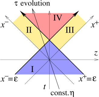
Figure 3: The source singularities are shifted by an infinitesimal amount $\epsilon$ in the $x^{+}$ and $x^{-}$ directions respectively. The $\tau$ integration from $0^{-}$ to $+\zeta$ is taken along a line of constant $\eta$. The backward light cone region corresponds to a negative $\tau$.

The main difficulty when dealing with the $\tau,\eta$ coordinates is that the (physical) singularity of the sources is located at the same position as the (unphysical) coordinate singularity at $\tau=0$. It should be noted that, while the backward light cone region is parameterized by a negative $\tau$, the difficulty stems from the impossibility to describe the space-like regions by a real $\tau$. We will introduce a regulator $\epsilon$, that we use to slightly shift the location of the sources. This helps to separate the physical singularities from the unphysical ones, as illustrated in Fig. 3. Then the space-time is divided into four regions,

$$\begin{array}[]{lp{0mm}@:p{2mm}l}\text{Region I}&&&x^{+}<\epsilon,\quad x^{-}<\epsilon,\\ \text{Region II}&&&0<x^{+}<\epsilon,\quad x^{-}>\epsilon,\\ \text{Region III}&&&0<x^{-}<\epsilon,\quad x^{+}>\epsilon,\\ \text{Region IV}&&&x^{+}>\epsilon,\quad x^{-}>\epsilon,\end{array}$$

separated by the source singularities. Let us consider the $\tau$ evolution along a line of constant $\eta$, e.g. in the negative $\eta$ region as illustrated in Fig. 3. Then the $\tau$ evolution first goes through a singularity at $x^{-}=\epsilon$ from the region I to the region II, and then through a second singularity at $x^{+}=\epsilon$ that leads to the region IV.

Equation (63) is trivial from Eq. (55). By inserting the canonical momenta into the Gauss law divided by $\tau$, we can get the following boundary condition,

$$\int_{0^{-}}^{\zeta}\!\mathrm{d}\tau\biggl{\{}\mathcal{D}_{i}\partial_{\tau}\mathcal{A}_{i}+\frac{1}{\tau^{2}}\partial_{\eta}\partial_{\tau}\mathcal{A}_{\eta}-\frac{\tau}{2}\biggl{[}\frac{1}{x^{+}}\rho_{1}\delta(x^{-}-\epsilon)+\frac{1}{x^{-}}\rho_{2}\delta(x^{+}-\epsilon)\biggr{]}\biggr{\}}=0\;,$$ (66)

where we perform this integration (66) with respect to $\tau$ in the small range from $0^{-}$ to $\zeta$ at fixed $\eta$. The upper bound $\tau=\zeta$ should be chosen such that $\zeta>\sqrt{2}\,\epsilon\,\mathrm{e}^{\eta}$ and $\zeta<\sqrt{2}\,\epsilon\,\mathrm{e}^{-\eta}$, so that the integration ends in the region II. Since only the singularity at $x^{-}=\epsilon$ is present on the integration path, we can assume that the background fields in the region II are proportional to the step function $\theta(x^{-}-\epsilon)$. Note that such a step function gives a delta function when differentiated with respect to $\tau$ or $\eta$. Let us therefore substitute the following forms,

$$\mathcal{A}_{i}=\alpha^{1}_{i}\theta(x^{-}-\epsilon)\quad,\quad\mathcal{A}_{\eta}=\tau^{2}\beta^{1}\theta(x^{-}-\epsilon)\;,$$ (67)

into Eq. (66). The only terms that survive in this integral in the limit $\epsilon\to 0^{+}$ are those containing a delta function. It should be noted that the $\mathcal{A}_{i}$ in the covariant derivative $\mathcal{D}_{i}$ drops out because it has the same color structure as $\partial_{\tau}\mathcal{A}_{i}$, as long as only the singular part is concerned (obtained when $\partial_{\tau}$ acts on the step function rather than on $\alpha^{1}_{i}$). After all, we get

$$\partial_{i}\alpha^{1}_{i}-2\beta^{1}-\rho_{1}=0\;.$$ (68)

The equation of motion (60) is then satisfied almost trivially, and the other equation of motion (61) leads to the very same boundary condition, and therefore we cannot determine uniquely $\alpha_{i}^{1}$ and $\beta_{1}$. This degeneracy is related to the residual gauge freedom; if we allow a nonzero $\beta^{1}$ proportional to $\rho_{1}$, then we can eliminate it by a gauge rotation applied to $\mathcal{A}_{\eta}$ without affecting the gauge condition $\mathcal{A}_{\tau}=0$ (except for terms of order $\tau\to 0$). We shall choose $\beta^{1}=0$ and therefore $\partial_{i}\alpha^{1}_{i}=\rho_{1}$. We can do the same for the region III, where we obtain the background $\mathcal{A}_{i}=\alpha^{2}_{i}\theta(x^{+}-\epsilon)$ with $\partial_{i}\alpha^{2}_{i}=\rho_{2}$.

Then, we shall push the time integration towards the region IV.  There is another singularity at $x^{+}=\epsilon$ for $\eta<0$ and at $x^{-}=\epsilon$ for $\eta>0$, which can be accounted for by using the following parameterization,

$$\mathcal{A}_{i}=\alpha^{1}_{i}\theta(x^{-}-\epsilon)\theta(\epsilon-x^{+})+\alpha^{2}_{i}\theta(x^{+}-\epsilon)\theta(\epsilon-x^{-})+\alpha^{3}_{i}\theta(x^{-}-\epsilon)\theta(x^{+}-\epsilon)\;,$$ (69)

where $\alpha^{1}_{i}$ and $\alpha^{2}_{i}$ are already fixed. If we differentiate twice with respect to $\tau$ or $\eta$ the products of theta functions in this expression, we obtain terms with two delta functions that are singular at $\tau=\eta=0$ (in the limit $\epsilon\to 0^{+}$). From the equation of motion (60), we therefore get the condition,

$$\int_{0^{-}}^{0^{+}}\mathrm{d}\eta\,\int_{0^{-}}^{\zeta}\mathrm{d}\tau\,\frac{1}{\tau}\partial_{\eta}^{2}\mathcal{A}_{i}=0\;,$$ (70)

where this time we must chose $\zeta>\sqrt{2}\,\epsilon\,\mathrm{e}^{\pm\eta}$ so that the endpoint of the $\tau$ integration is in the region IV.  This relation leads to

$$\alpha^{3}_{i}=\alpha^{1}_{i}+\alpha^{2}_{i}\;.$$ (71)

Let us finally perform the integration (66) with the ansatz

$$\mathcal{A}_{\eta}=\tau^{2}\beta^{3}\theta(x^{+}-\epsilon)\theta(x^{-}-\epsilon)\;.$$ (72)

In this case, it is important to note that $\partial_{\tau}\mathcal{A}_{i}$ can have a different color structure than that of $\mathcal{A}_{i}$. Therefore, we should keep the covariant derivative $\mathcal{D}_{i}$ and treat carefully the commutators such as $[\mathcal{A}_{i},\partial_{\tau}\mathcal{A}_{i}]$ and $[\mathcal{A}_{i},\partial_{\eta}\mathcal{A}_{i}]$. The Gauss law (66) eventually leads to the boundary condition

$$\partial_{i}\alpha^{1}_{i}+\partial_{i}\alpha^{2}_{i}-\mathrm{i}g[\alpha^{1}_{i},\alpha^{2}_{i}]+2\beta^{3}-\rho_{1}-\rho_{2}=0\;,$$ (73)

and the equation of motion (61) gives again the same condition, which results in

$$\beta^{3}=\frac{\mathrm{i}g}{2}\;[\alpha^{1}_{i},\alpha^{2}_{i}]\;.$$ (74)

Hence, one can reproduce the classical background fields (62)-(65) in the $\tau,\eta$ coordinates by slightly shifting the source singularities. We should emphasize here that, even though we have $\mathcal{E}^{i}=0$, we must keep terms such as $\partial_{\tau}\mathcal{E}^{i}$ and $\tau^{-1}\mathcal{E}^{i}$ which are non-vanishing when $\tau\to 0$. Since $\mathcal{A}_{\eta}$, in contrast, goes to zero like $\mathcal{O}(\tau^{2})$, we can drop $\partial_{\tau}\mathcal{A}_{\eta}=0$ and $\tau^{-1}\mathcal{A}_{\eta}=0$ in the limit $\tau\to 0$.

4.4 Wavefunction in the backward light cone region

We now proceed with the derivation of the wavefunction in the $\tau,\eta$ coordinates in the non-Abelian gauge theory. Let us first consider the backward light cone region in the weak coupling regime. We see that $A_{\eta}$ and $E^{\eta}$ are not a dynamical variables on the light cone in the $A_{\tau}=0$ gauge. Therefore, the wavefunction does not involve $A_{\eta}$ at all and the Gauss law provides $E^{\eta}$ as a function of the dynamical variables. In other words, $E^{\eta}$ is a solution of the Gauss law with $A_{\eta}=0$ substituted,

$$E^{\eta}=-\frac{1}{\partial_{\eta}}D_{i}E^{i}\;,$$ (75)

where we should remark that the fields and the momenta in this identity are the full ones, including both the classical backgrounds and the quantum fluctuations.

In the following, we denote the quantum fluctuations with lowercase letters,

$$a_{i}\equiv A_{i}-\mathcal{A}_{i}\;,\quad a_{\eta}\equiv A_{\eta}-\mathcal{A}_{\eta}\;,\quad e^{i}\equiv E^{i}-\mathcal{E}^{i}\;,\quad e^{\eta}\equiv E^{\eta}-\mathcal{E}^{\eta}\;.$$ (76)

We then expand the Hamiltonian to quadratic order in the fluctuations, and then the time-independent Schrödinger equation can be written as

$$\begin{split}&\int\mathrm{d}\eta\,\mathrm{d}^{2}{\boldsymbol{x}}_{\perp}\,\mathrm{tr}\biggl{\{}-\frac{1}{\tau}\frac{\delta^{2}}{\delta a_{i}^{2}}-\tau\frac{\delta^{2}}{\delta a_{\eta}^{2}}+\frac{1}{\tau}(\partial_{\eta}a_{i}-\mathcal{D}_{i}a_{\eta})^{2}\\ &\qquad+\frac{\tau}{2}\Bigl{[}(\mathcal{D}_{i}a_{j}-\mathcal{D}_{j}a_{i})^{2}-2\mathrm{i}g\mathcal{F}_{ij}[a_{i},a_{j}]\Bigr{]}\biggr{\}}\Psi_{-}[A]=E\Psi_{-}[A]\;,\end{split}$$ (77)

with an energy eigenvalue $E$. When writing this Schrödinger equation, we have replaced the canonical momenta by differential operators, thanks to the canonical commutation relations at equal $\tau$,

$$\bigl{[}a_{i}^{a}(\eta,{\boldsymbol{x}}_{\perp}),e^{jb}(\eta^{\prime},{\boldsymbol{x}}_{\perp}^{\prime})\bigr{]} =\mathrm{i}\delta^{ab}\delta^{ij}\delta(\eta-\eta^{\prime})\delta^{(2)}({\boldsymbol{x}}_{\perp}-{\boldsymbol{x}}_{\perp}^{\prime})\;,$$ (78)

$$\bigl{[}a_{\eta}^{a}(\eta,{\boldsymbol{x}}_{\perp}),e^{\eta b}(\eta^{\prime},{\boldsymbol{x}}_{\perp}^{\prime})\bigr{]} =\mathrm{i}\delta^{ab}\delta(\eta-\eta^{\prime})\delta^{(2)}({\boldsymbol{x}}_{\perp}-{\boldsymbol{x}}_{\perp}^{\prime})\;.$$ (79)

It should be mentioned here that the right hand side does not involve $\tau$ explicitly because we have defined the canonical momenta $e^{i}$ and $e^{\eta}$ from $\tau H$, including the measure.

Changing temporarily to the variables $a_{\zeta}\equiv a_{\eta}/\tau$ (and $\partial_{\eta}\equiv\tau\partial_{\zeta}$), and using the notation $a_{{}_{I}}\equiv(a_{i},a_{\zeta})$, we can write the Schrödinger equation in the following compact form,

$$\int\mathrm{d}\eta\,\mathrm{d}^{2}{\boldsymbol{x}}_{\perp}\,\mathrm{tr}\biggl{[}-\frac{1}{\tau}\frac{\delta^{2}}{\delta a_{{}_{I}}^{2}}+\tau\,a_{{}_{I}}\cdot G^{-1}_{{}_{IJ}}\cdot a_{{}_{J}}\biggr{]}\Psi_{-}[A]=E\Psi_{-}[A]\;,$$ (80)

where we have defined the background propagator,

$$(G^{-1}_{{}_{IJ}})^{ab}\equiv-\delta_{{}_{IJ}}(\mathcal{D}^{2})^{ab}+(\mathcal{D}_{{}_{I}}\mathcal{D}_{{}_{J}})^{ab}-2gf^{acb}\mathcal{F}_{{}_{IJ}}^{c}\;,$$ (81)

with $\mathcal{D}^{2}\equiv\partial_{\zeta}^{2}+\mathcal{D}_{i}\mathcal{D}_{i}$. The formal solution to this Schrödinger equation is not difficult to find. The ground state solution to Eq. (77) or Eq. (80) can be expressed in terms of the square-root of the inverse propagator $G^{-1}$ as

$$\Psi_{-}=N\exp\biggl{[}-\int\mathrm{d}\eta\,\mathrm{d}^{2}{\boldsymbol{x}}_{\perp}\,\tau\,\mathrm{tr}\Bigl{(}a_{{}_{I}}\,\sqrt{G^{-1}_{{}_{IJ}}}\,a_{{}_{J}}\Bigr{)}\biggr{]}\;,$$ (82)

where we have chosen only the normalizable solution. Since there is no background field in the backward light cone region, the square-root of the inverse propagator is easy to calculate. It is simply proportional to the transverse projection operator $\delta_{{}_{IJ}}-\partial_{{}_{I}}\partial_{{}_{J}}/\partial^{2}$. Noting that $a_{\zeta}=\tau^{-1}a_{\eta}\to 0$, we see that the wavefunction is simply

$$\Psi_{-}[A]=N\exp\Biggl{\{}\!-\!\!\int\!\mathrm{d}\eta\,\mathrm{d}^{2}{\boldsymbol{x}}_{\perp}\,\mathrm{tr}\biggl{[}a_{i}\,\tau\sqrt{\!-\left(\frac{\partial_{\eta}}{\tau}\right)^{2}\!-\!{\boldsymbol{\partial}}_{\perp}^{2}}\,\Bigl{(}\delta_{ij}-\frac{\partial_{i}\partial_{j}}{(\frac{\partial_{\eta}}{\tau})^{2}+{\boldsymbol{\partial}}_{\perp}^{2}}\Bigr{)}a_{j}\biggr{]}\Biggr{\}}\;.$$ (83)

Except when $\partial_{\eta}$ is smaller than $\tau Q_{s}$, the $\partial_{\eta}/\tau$ term dominates over the transverse derivative. For the analysis of the instability, however, we may have to retain the transverse momentum here, because the unstable $\eta$ dependent modes may be very soft [11]. Also we note that, although we have used the notation $a_{i}$, it is identical to the full fields $A_{i}$ in the absence of backgrounds in the backward light cone region.

4.5 Singularity in the Hamiltonian

In order to clarify the boundary condition at the source singularity, we first need the Hamiltonian in the presence of background fields, and more specifically its singularity. Note that the singular part of the Hamiltonian should commute with the Gauss law because of gauge invariance.

The explicit form of the Hamiltonian in the presence of the background reads

$$\tau\mathcal{H}=\mathrm{tr}\biggl{[}\frac{1}{\tau}e^{i}e^{i}+\frac{2}{\tau}\mathcal{E}^{i}e^{i}+\frac{1}{\tau}\mathcal{E}^{i}\mathcal{E}^{i}+\tau e^{\eta}e^{\eta}+2\tau\mathcal{E}^{\eta}e^{\eta}+\tau\mathcal{E}^{\eta}\mathcal{E}^{\eta}$$

$$+\frac{1}{\tau}\bigl{(}\partial_{\eta}a_{i}-\mathcal{D}_{i}a_{\eta})^{2}-\frac{2}{\tau}\mathrm{i}g\,(\partial_{\eta}\mathcal{A}_{i})[a_{\eta},a_{i}]+\frac{2}{\tau}(\partial_{\eta}\mathcal{A}_{i})(\partial_{\eta}a_{i}-\mathcal{D}_{i}a_{\eta})+\frac{1}{\tau}(\partial_{\eta}\mathcal{A}_{i})^{2}$$

$$\quad+\frac{\tau}{2}\bigl{(}\mathcal{D}_{i}a_{j}-\mathcal{D}_{j}a_{i}\bigr{)}^{2}-\tau\mathrm{i}g\,\mathcal{F}_{ij}[a_{i},a_{j}]+\tau\,\mathcal{F}_{ij}(\partial_{i}a_{j}-\partial_{j}a_{i})+\frac{\tau}{2}\mathcal{F}_{ij}^{2}$$

$$\qquad+\tau\Bigl{\{}\frac{1}{x^{+}}\rho_{1}\,\delta(x^{-})-\frac{1}{x^{-}}\rho_{2}\,\delta(x^{+})\Bigr{\}}a_{\eta}\biggr{]}\;,$$ (84)

up to quadratic order in the fluctuations. The last term is the current density due to the sources, which can also be expressed as $J^{\eta}=-(2/\tau)\partial_{i}\partial_{\eta}\mathcal{A}_{i}$. Gauge invariance requires the covariant conservation of the current, i.e. $D_{\eta}J^{\eta}=0$, which is actually satisfied thanks to Eq. (70), since $A_{\eta}\to 0$ at $\tau\to 0$ .

Thus, in the limit $a_{\eta}\to 0$, the singular terms in the Hamiltonian are

$$\tau\mathcal{H}_{\text{sing}}=\mathrm{tr}\biggl{[}\,2(\partial_{\tau}\mathcal{A}_{i})e^{i}+\frac{2}{\tau}(\partial_{\eta}\mathcal{A}_{i})(\partial_{\eta}a_{i})+\frac{1}{\tau}(\partial_{\eta}\mathcal{A}_{i})^{2}\biggr{]}\;.$$ (85)

Here we have used Eq. (57) in order to rearrange the first term. The delta-function singularities originate from $\partial_{\eta}$ and $\partial_{\tau}$ acting on the step function in $\mathcal{A}_{i}$. The second and third terms can be in fact dropped thanks to Eq. (70), after an integration by parts. Therefore, the only remaining singular term is after all,

$$\tau\mathcal{H}_{\text{sing}}=2\mathrm{tr}\bigl{[}\,(\partial_{\tau}\mathcal{A}_{i})e^{i}\bigr{]}\;,$$ (86)

on the light cone where $a_{\eta}$ is vanishing.

4.6 In the forward light cone region

By integrating the Schrödinger equation with respect to $\tau$ from $0^{-}$ to $\zeta$ with the singularity in the Hamiltonian we have just identified in Eq. (86), we can derive a relation between the wavefunctions in the infinitesimally backward and forward light cone regions.

In principle, we can follow the same procedure as the one used for the determination of the classical backgrounds. By shifting the singularities as shown in Fig. 3, we can access the space-like regions while using the $\tau,\eta$ coordinates. In the presence of the regulator $\epsilon$, we should keep $A_{\eta}$ terms which are of order $\epsilon^{2}$, and the $\tau$ integration from I towards IV will pick up singular terms proportional to $A_{\eta}$. When the wavefunction contains linear terms in $A_{\eta}$ in the exponential, the $A_{\eta}$ integration in the Wigner transformation results in the delta-function constraint imposed on the conjugate variable $E^{\eta}$. At the end in the limit of $\epsilon\to 0$, we must take simultaneously the limit $A_{\eta}\to 0$, so that the $A_{\eta}$ terms in the wavefunction disappear. Nevertheless the constraint on $E^{\eta}$ preserves some information about the singular terms. This procedure is a bit tedious to implement, but the final answer is quite simple: the Gauss law always holds, from which one can obtain $E^{\eta}$ as a function of the other fields. Therefore, the constraint on $E^{\eta}$ after the $A_{\eta}$ integration simply coincides with the Gauss law (59). This means that we can obtain the final answer by the following shortcut: drop all the singular terms involving $A_{\eta}$ and add by hand to the Wigner function a delta-function constraint fixing $E^{\eta}$ from the Gauss law.

Since we can set $A_{\eta}=0$ even with finite $\epsilon$, the singular Hamiltonian (86) is sufficient for our purpose to connect the wavefunctions between the two light-cones. The Schrödinger equation leads to the boundary condition from $\tau=0^{-}$ to $\tau=\zeta\to 0^{+}$,

$$\mathrm{i}(\Psi_{+}-\Psi_{-})=\Bigl{(}\int_{0^{-}}^{\zeta}\!\mathrm{d}\tau\int\mathrm{d}\eta\,\mathrm{d}^{2}{\boldsymbol{x}}_{\perp}\,\tau\mathcal{H}_{\text{sing}}\Bigr{)}\frac{1}{2}(\Psi_{+}+\Psi_{-})\;.$$ (87)

Neglecting higher order terms in the fluctuations, we can solve the above equation as

$$\Psi_{+}\simeq\exp\biggl{[}-\mathrm{i}\int_{0^{-}}^{\zeta}\!\mathrm{d}\tau\int\mathrm{d}\eta\,\mathrm{d}^{2}{\boldsymbol{x}}_{\perp}\,\tau\mathcal{H}_{\text{sing}}\biggr{]}\Psi_{-}\;,$$ (88)

where $\tau\mathcal{H}_{\text{sing}}$ is given by Eq. (86). The identification of $e^{i}$ as the differential operator $-\mathrm{i}\delta/\delta A_{i}$ enables us to write

$$\int_{0^{-}}^{\zeta}\!\mathrm{d}\tau\,\tau\mathcal{H}_{\text{sing}}=2\mathrm{tr}\bigl{[}\mathcal{A}_{i}(\zeta)\,e^{i}\bigr{]}=-\mathrm{i}\mathcal{A}_{i}^{a}(\zeta)\frac{\delta}{\delta A_{i}^{a}}\;.$$ (89)

The exponential of this differential operator is nothing but the translation operator of $A_{i}$ by an amount $-\mathcal{A}_{i}$ ; i.e. $A_{i}\to A_{i}-\mathcal{A}_{i}$. Therefore, we conclude that $\Psi_{+}[A]=\Psi_{-}[A-\mathcal{A}]$. By taking the limit $\epsilon\to 0^{+}$ while keeping the final time $\zeta$ very small but fixed, the surface of constant time $\tau=\zeta$ lies entirely in the region IV, where the classical transverse field is $\mathcal{A}_{i}=\alpha^{1}_{i}+\alpha^{2}_{i}$. Thus, we finally obtain the following wavefunction in the forward light-cone,

$$\Psi_{+}[A]=\Psi_{-}[A-(\alpha^{1}+\alpha^{2})]\;,$$ (90)

with the wavefunction defined in Eq. (83).

Although the wavefunction takes the same functional form, it is the Gauss law which is actually affected nontrivially by the source singularity, and the fluctuations in $e^{\eta}$ are uniquely fixed from the background fields (62) and (65), and the fluctuations $a_{i}$ and $e^{i}$. Namely, from Eq. (75), up to term of quadratic order in fluctuations, we have

$$e^{\eta}=e^{\eta}_{0}-\int_{\eta_{0}}^{\eta}\mathrm{d}\eta\;\mathcal{D}_{i}e^{i}\;,$$ (91)

where we assumed that the fluctuation $e^{i}$ does not contain a singularity of the type $\sim\tau\partial_{\tau}\theta(x^{\pm}-\epsilon)$ (unlike the classical transverse electric field $\mathcal{E}^{i}$ – The $\eta$ integration of $\mathcal{D}_{i}\mathcal{E}^{i}$ leads to $\mathcal{E}^{\eta}$ because of this singularity.) The origin of the presence of an indefinite integral constant $e^{\eta}_{0}$ is that the Gauss law cannot constrain the $\eta$ zero-mode of $e^{\eta}$. In such a case, the $a_{\eta}$ integration in the Wigner transform would impose the zero-mode to vanish. Hence, $e^{\eta}_{0}$ should be fixed by the condition $\int_{-\infty}^{\infty}\!\mathrm{d}\eta\,e^{\eta}=0$.

4.7 Wigner transformation

Finally, we can compute the Wigner function from the wavefunction. The conditions of $a_{\eta}\to 0$ and the Gauss law constraint are, as we have noted before, expressed by delta-functions added by hand. We can then write the Wigner function as follows :

$$W[a,e]$$

$$=N\int\big{[}\mathrm{d}\delta a\big{]}\;\Psi_{+}^{\ast}[a-\textstyle\frac{1}{2}\delta a]\,\Psi_{+}[a+\textstyle\frac{1}{2}\delta a]\,\mathrm{e}^{-\mathrm{i}\int\mathrm{d}\eta\,\mathrm{d}^{2}{\boldsymbol{x}}_{\perp}\,2\mathrm{tr}[e^{i}\delta a_{i}]}$$

$$=N\exp\Biggl{\{}-\int\mathrm{d}\eta\,\mathrm{d}^{2}{\boldsymbol{x}}_{\perp}\,2\mathrm{tr}\biggl{[}a_{i}\,\tau\sqrt{-(\partial_{\eta}/\tau)^{2}-{\boldsymbol{\partial}}_{\perp}^{2}}\,\Bigl{(}\delta_{ij}-\frac{\partial_{i}\partial_{j}}{(\partial_{\eta}/\tau)^{2}+{\boldsymbol{\partial}}_{\perp}^{2}}\Bigr{)}\,a_{j}$$

$$\qquad+e^{i}\frac{1}{\tau\sqrt{-(\partial_{\eta}/\tau)^{2}-{\boldsymbol{\partial}}_{\perp}^{2}}}\,\Bigl{(}\delta_{ij}+\frac{\partial_{i}\partial_{j}}{(\partial_{\eta}/\tau)^{2}}\Bigr{)}\,e^{j}\biggr{]}\Biggr{\}}$$

$$\qquad\qquad\times\delta[a_{\eta}]\,\delta\biggl{[}e^{\eta}-e^{\eta}_{0}+\int_{\eta_{0}}^{\eta}\mathrm{d}\eta\;\mathcal{D}_{i}e^{i}\biggr{]}\;,$$ (92)

where $\delta_{ij}+\partial_{i}\partial_{j}/(\partial_{\eta}/\tau)^{2}$ is the inverse of $\delta_{ij}-\partial_{i}\partial_{j}/[(\partial_{\eta}/\tau)^{2}+{\boldsymbol{\partial}}_{\perp}^{2}]$. This Wigner function allows us to compute the average of any observable $\mathcal{O}[A]$ at later time $\tau>0$ with initial quantum fluctuations, as follows,

$$\langle\mathcal{O}\rangle_{\tau}=\int\big{[}\mathrm{d}a_{i}\,\mathrm{d}a_{\eta}\,\mathrm{d}e^{i}\,\mathrm{d}e^{\eta}\big{]}\;W[a,e]\;\mathcal{O}\bigl{[}\mathcal{A}[\mathcal{A}_{i}+a_{i},a_{\eta},e^{i},\mathcal{E}^{\eta}+e^{\eta};\tau]\bigr{]}\;.$$ (93)

Here we symbolically denote by $\mathcal{A}[\mathcal{A}_{i}+a_{i},a_{\eta},e^{i},\mathcal{E}^{\eta}+e^{\eta};\tau]$ the classical gauge field obtained at time $\tau$ by solving the classical equations of motion (60) and (61) with initial conditions $\mathcal{A}_{i}+a_{i}$, $a_{\eta}$, $e^{i}$, and $\mathcal{E}^{\eta}+e^{\eta}$ at $\tau=0^{+}$, where $\mathcal{A}_{i}$ and $\mathcal{E}^{\eta}$ are the usual background fields (62) and (65) respectively.

The Gaussian Wigner function describes the dispersion of fluctuations around the classical initial condition. The distribution turns out not to be of white-noise type but to be characterized by the correlation function,

$$\bigl{\langle}a_{i}(\eta,{\boldsymbol{x}}_{\perp})\,a_{j}(\eta^{\prime},{\boldsymbol{x}}_{\perp}^{\prime})\bigr{\rangle}=\frac{\displaystyle\int\big{[}\mathrm{d}a_{i}\,\mathrm{d}a_{\eta}\,\mathrm{d}e^{i}\,\mathrm{d}e^{\eta}\big{]}\;W[a,e]\;a_{i}(\eta,{\boldsymbol{x}}_{\perp})\,a_{j}(\eta^{\prime},{\boldsymbol{x}}_{\perp}^{\prime})}{\displaystyle\int\big{[}\mathrm{d}a_{i}\,\mathrm{d}a_{\eta}\,\mathrm{d}e^{i}\,\mathrm{d}e^{\eta}\big{]}\;W[a,e]}$$

$$=\frac{1}{\tau\sqrt{-(\partial_{\eta}/\tau)^{2}-{\boldsymbol{\partial}}_{\perp}^{2}}}\Bigl{(}\delta_{ij}+\frac{\partial_{i}\partial_{j}}{(\partial_{\eta}/\tau)^{2}}\Bigr{)}\,\delta(\eta-\eta^{\prime})\,\delta^{(2)}({\boldsymbol{x}}_{\perp}\!-\!{\boldsymbol{x}}_{\perp}^{\prime})\;.$$ (94)

The fluctuation of canonical momenta is characterized inversely by

$$\begin{split}&\bigl{\langle}e^{i}(\eta,{\boldsymbol{x}}_{\perp})\,e^{j}(\eta^{\prime},{\boldsymbol{x}}_{\perp}^{\prime})\bigr{\rangle}\\ &=\tau\sqrt{-(\partial_{\eta}/\tau)^{2}-{\boldsymbol{\partial}}_{\perp}^{2}}\Bigl{(}\delta_{ij}-\frac{\partial_{i}\partial_{j}}{(\partial_{\eta}/\tau)^{2}+{\boldsymbol{\partial}}_{\perp}^{2}}\Bigr{)}\,\delta(\eta-\eta^{\prime})\,\delta^{(2)}({\boldsymbol{x}}_{\perp}\!-\!{\boldsymbol{x}}_{\perp}^{\prime})\;.\end{split}$$ (95)

The formula (93) and the above two relations, Eqs. (94) and (95), are our central result. Regarding the $\eta$ components, $a_{\eta}$ is vanishing while $e^{\eta}$ is fixed by the Gauss law. In the limit of $\tau\to 0$ the distribution becomes simpler, and depends solely on the derivative with respect to rapidity, $\partial_{\eta}$. For practical uses, however, it is not possible to start the numerical simulation exactly at $\tau=0^{+}$, and the transverse derivatives ${\boldsymbol{\partial}}_{\perp}$ will then play the role of a regulator for infrared modes when $\partial_{\eta}/\tau$ is smaller than ${\boldsymbol{\partial}}_{\perp}$.

5 Conclusions

In this paper, we have discussed an approximation scheme for calculating the quantum expectation value of an observable that depends on field configurations at late times. In the WKB approximation, we have obtained a formula giving this expectation value from the classical equations of motion, with an initial condition that includes fluctuations. The spectrum of these initial fluctuations is specified by the Wigner transform of the wavefunction, the latter being obtained as a ground state solution of the Schrödinger equation. Our formula is generic enough that we can expect a variety of applications, for instance to the study of an unstable system, or to that of the spinodal decomposition associated with a phase transition.

An application of particular interest to heavy ion collisions is to calculate the Wigner function of these fluctuations immediately after the initial impact of the two nuclei, in the weak coupling regime. These initial quantum fluctuations provide the seeds that trigger the instability of the rapidity dependent modes. The precise determination of initial fluctuations or seeds is of crucial importance for the estimate of the growth rate of the unstable modes.

By identifying the physically relevant gauge fluctuations and the singularity in the Hamiltonian density, we have derived the discontinuity between the wavefunctions in the backward and forward light-cones. It turns out that the initial singularity results only in a shift in the transverse gauge fields, equal to the classical background field. This is because, on the light-cone, the physical degrees of freedom are gauge fields polarized in the perpendicular plane and the longitudinal mode along the collision axis has to vanish.

This wavefunction and the resultant Wigner function describe the spectrum of initial fluctuations. There are two noteworthy features in our results.

Firstly, both $e^{i}$ and $a_{i}$ fluctuate, with 2-point correlations that are inversely related to one another. This means, if the boost invariance is largely violated by $e^{i}$, then $a_{i}$ fluctuations are suppressed, and vice versa. Thus, the prescription adopted in Ref. [11], in which only the $e^{i}$ fluctuations are taken into account, needs to be extended in order to include also the fluctuations of $a_{i}$. It should be important to describe these fluctuations correctly because the $a_{i}$ distribution rather than $e^{i}$ distribution has large correlation for infrared modes having a small rapidity dependence.

Secondly, although it may be less important, the off-diagonal correlation between $x$ and $y$ components is not vanishing. Again, this might be relevant for infrared modes. This feature is also missing in Ref. [11].

It would be interesting to see how these modifications of the fluctuation spectrum affect the growth rate of the instability. Although the spectrum of the initial fluctuations could be obtained analytically, this question can only be investigated numerically, since it requires to solve the classical Yang-Mills equations in the forward light-cone.

6 Acknowledgments

We thank Raju Venugopalan and Tuomas Lappi for useful discussions and Sangyong Jeon for comments. This work was supported in part by the RIKEN BNL Research Center and the U.S. Department of Energy under cooperative research agreement #DE-AC02-98CH10886. FG would like to thank the Institute of Nuclear Theory at the University of Washington for its hospitality and financial support while this work was being completed.

References

• [1] L. D. McLerran and R. Venugopalan, Phys. Rev. D49 (1994) 2233; 3352; D50 (1994) 2225.
• [2] J. Jalilian-Marian, A. Kovner, L. McLerran and H. Weigert, Phys. Rev. D55 (1997) 5414.
• [3] J. Jalilian-Marian, A. Kovner, A. Leonidov and H. Weigert, Nucl. Phys. B504 (1997) 415; Phys. Rev. D59 (1999) 014014.
• [4] E. Iancu and L. McLerran, Phys. Lett. B510 (2001) 145.
• [5] E. Iancu, A. Leonidov and L. D. McLerran, Nucl. Phys. A692 (2001) 583; E. Ferreiro E. Iancu, A. Leonidov and L. D. McLerran, Nucl. Phys. A703 (2002) 489.
• [6] A. Kovner, L. McLerran and H. Weigert, Phys. Rev. D52 (1995) 3809; 6231.
• [7] A. Krasnitz and R. Venugopalan, Nucl. Phys. B557 (1999) 237; Phys. Rev. Lett. 84 (2000) 4309; Phys. Rev. Lett. 86 (2001) 1717.
• [8] A. Krasnitz, Y. Nara and R. Venugopalan, Phys. Rev. Lett. 87 (2001) 192302; Nucl. Phys. A717 (2003) 268; A727 (2003) 427.
• [9] T. Lappi, Phys. Rev. C67 (2003) 054903.
• [10] T. Lappi and L. McLerran, Nucl. Phys. A772 (2006) 200.
• [11] P. Romatschke and R. Venugopalan, Phys. Rev. Lett. 96 (2006) 062302; Eur. Phys. J. A29 (2006) 71; Phys. Rev. D74 (2006) 045011.
• [12] S. Mrowczynski, Phys. Lett. B214 (1988) 587; B314 (1993) 118; B393 (1997) 26; S. Mrowczynski, A. Rebhan and M. Strickland, Phys. Rev. D70 (2004) 025004.
• [13] P. Arnold, J. Lenaghan and G. Moore, JHEP 0308 (2003) 002; P. Arnold, J. Lenaghan, G. Moore and L. Yaffe, Phys. Rev. Lett. 94 (2005) 072302.
• [14] P. Romatschke and M. Strickland, Phys. Rev. D68 (2003) 036004; D70 (2004) 116006. A. Rebhan, P. Romatschke and M Strickland, Phys. Rev. Lett. 94 (2005) 102303; JHEP 0509 (2005) 041, P. Romatschke and A. Rebhan, hep-ph/0605064.
• [15] P. Arnold, J. Lenaghan, G. D. Moore and L. G. Yaffe, Phys. Rev. Lett. 94 (2005) 072302; P. Arnold, G. D. Moore and L. G. Yaffe, Phys. Rev. D72 (2005) 054003.
• [16] P. Arnold and G. D. Moore, Phys. Rev. D73 (2006) 025006; 025013.
• [17] D. Bodeker, JHEP 0510 (2005) 092.
• [18] A. Dumitru and Y. Nara, Phys. Lett. B621 (2005) 89.
• [19] A. Dumitru, Y. Nara and M. Strickland, hep-ph/0604149.
• [20] B. Schenke, M. Strickland, C. Greiner and M. H. Thoma, Phys. Rev. D73 (2006) 125004.
• [21] J. Randrup and S. Mrowczynski, Phys. Rev. C68 (2003) 034909; S. Mrowczynski, Acta Phys. Polon. B37 (2006) 427.
• [22] R. Baier, A. H. Mueller, D. Schiff and D. T. Son, Phys. Lett. B502 (2001) 51.
• [23] D. Kharzeev, A. Krasnitz and R. Venugopalan, Phys. Lett. B545 (2002) 298.
• [24] A. H. Mueller, A. I. Shoshi and S. M. H. Wong, hep-ph/0607136.
• [25] A. H. Mueller and D. T. Son, Phys. Lett. B582 (2004) 279.
• [26] S. Jeon, Phys. Rev. C72 (2005) 014907.
• [27] F. Gelis and R. Venugopalan, Nucl. Phys. A776 (2006) 135; Nucl. Phys. A779 (2006) 177.
• [28] F. Gelis, K. Kajantie and T. Lappi, Phys. Rev. C71 (2005) 024904; Phys. Rev. Lett. 96 (2006) 032304.
• [29] F. Gelis, T. Lappi and R. Venugopalan, work in progress.
• [30] D, Kharzeev and K. Tuchin, Nucl. Phys. A753 (2005) 316; Phys. Lett. B626 (2005) 147; D. Kharzeev, E. levin and K. Tuchin, hep-ph/0602063.
• [31] G. Barton, Annals Phys. 166 (1986) 322.
• [32] D. T. Son, hep-ph/9601377; S. Y. Khlebnikov and I. I. Tkachev, Phys. Rev. Lett. 77 (1996) 219; F. Cooper, S. Habib, Y. Kluger and E. Mottola, Phys. Rev. D55 (1997) 6471.