$l\rightarrow l^{\prime}\gamma$ in the Lepton Number Violating MSSM
Steven Rimmer
Institute for Particle Physics Phenomenology (IPPP), Durham DH1 3LE, UK

ABSTRACT

A minimal particle content supersymmetric model with a discrete ${\cal Z}_{3}$ symmetry, allowing lepton number violating terms, is studied. Within this model, the neutrino masses and mixing can be generated by lepton number violating couplings. Choosing parameters which correctly describe both the masses and mixing in the neutrino sector, we consider their repercussions in flavour violating radiative lepton decays, $l\rightarrow l^{\prime}\gamma$. Such decays have not been observed and, accordingly, soon to be improved, upper bounds on their branching ratios exist. We do not assume dominance of either the bilinear or trilinear couplings. We note that certain parameter sets, which correctly describe the neutrino sector, will also generate observable branching ratios, some of which are already precluded, and suggest four such sets as Benchmark scenarios.

1 Introduction

Processes which do not conserve lepton flavour, the flavour oscillations in the neutrino sector, have been observed [1]. This is in contrast with the charged sector, where no such observation has been made. The decays $\tau\rightarrow\mu\gamma,e\gamma$ and $\mu\rightarrow e\gamma$ can be driven solely by the known lepton flavour violation in the neutral sector, the branching ratio will be small [2], however, well below current experimental limits, due to the magnitude of the neutrino mass. Noticing that in many extensions of the Standard Model this branching ratio increases greatly, together with the fact that experimental bounds for these decays will soon be improved by several orders of magnitude, suggests that these decays are a valuable place to scrutinise the Standard Model and test theories which extend it.

The model considered here, the Lepton Number Violating Minimal Supersymmetric Standard Model (/L-MSSM), is a well motivated extension of the Standard Model. When constructing a supersymmetric model dangerous operators arise which, unless highly suppressed, would give rise to an unacceptable rate for proton decay. As such, a discrete symmetry must be imposed when constructing the Lagrangian [10, 11]. We choose a discrete symmetry which allows lepton number violating terms, but not baryon number violating terms, resulting in proton stability. The lepton number violating terms violate R-parity. The superpotential for the /L-MSSM is given by

$${\cal W}_{\rm\leavevmode\nobreak\ {/}L-MSSM}=\epsilon_{ab}\left(\frac{1}{2}\lambda_{\alpha\beta k}{\cal L}_{\alpha}^{a}{\cal L}_{\beta}^{b}\bar{E}_{k}\>+\>\lambda^{\prime}_{\alpha jk}{\cal L}_{\alpha}^{a}Q_{j}^{b,x}\bar{D}_{k,x}\>+\>(Y_{U})_{jk}Q_{j}^{a,x}H_{2}^{b}\bar{U}_{k,x}\>-\>\mu_{\alpha}{\cal L}_{\alpha}^{a}H_{2}^{b}\right),$$

(1.1)

where $Q_{i}^{a\,x},\;{\bar{D}}_{i}^{x},\;{\bar{U}}_{i}^{x},\;{\cal L}_{i}^{a},\;{\bar{E}}_{i},\;H_{1}^{a},\;H_{2}^{a}$ are the chiral superfield particle content, $i=1,2,3$ is a generation index, $x=1,2,3$ and $a=1,2$ are $SU(3)$ and $SU(2)$ gauge indices, respectively. ${\cal L}^{a}_{\alpha=0,\ldots,3}=(H_{1}^{a},\,L_{i=1,2,3}^{a})$ and hence, $\lambda_{0jk}$ are the lepton Yukawa couplings and $\lambda_{ijk}$ are lepton number violating parameters, whose role will be considered later. $\mu_{\alpha}$ is the generalised dimensionful $\mu$-parameter, with $\mu_{0}$ and $\mu_{i}$, $i=1,...3$ the lepton number conserving and violating parts respectively. Similarly, $\lambda^{\prime}_{0jk}$ are the Yukawa couplings for the down-type quarks and $\lambda^{\prime}_{ijk}$ violate lepton number. Finally, $(Y_{U})_{ij}$ are Yukawa matrices with $\epsilon_{ab}$ being the totally anti-symmetric tensor $\epsilon_{12}=+1$. The are further sources of lepton number violation in the soft breaking sector, however, we present here merely the terms which will play a role in this paper,

$$\mathcal{L}_{\rm SSB}\supset B_{\alpha}\tilde{\nu}^{\phantom{*}}_{L\alpha}h_{2}^{0}-B_{\alpha}\tilde{e}^{\phantom{*}}_{L\alpha}h_{2}^{+}\;\;+\;\textup{H. c.}\;\;,$$ (1.2)

where $B_{\alpha}$ is the four-component bilinear term $B_{\alpha}=(B_{0},B_{i})$ are $B_{i}$ are the lepton number violating components. The full supersymmetry breaking part of the Lagrangian and the mass matrices along with further details of the model are presented in Refs. [12, 13]. The calculation is performed in a basis where the vacuum expectation values for the sneutrinos are zero; a method for moving to this basis from the most general scalar potential and properties of this basis are outlined in Ref. [14].

A particularly noteworthy feature is that the current experimental values of neutrino mass squared differences and mixing can be accommodated within the model, being determined by the value of lepton number violating couplings in either the superpotential, or the supersymmetry breaking terms of the Lagrangian [13]. In fact it has been shown that, one, and only one, neutrino mass can be generated at tree-level [15, 16, 17, 18] with the masses of the two remaining generations arising through radiative corrections, producing the hierarchy between solar and atmospheric mass differences in a convenient fashion. Furthermore, this scenario can arise from a Froggatt-Nielsen model in which the discrete symmetry is due to the breaking of a $U(1)_{X}$ [19].

Crucially, the operators which give rise to neutrino masses in this model may also give rise to lepton flavour violation in the charged sector. In this paper, we shall consider combinations of lepton number violating parameters that correctly reproduce the observations made in oscillation experiments. For these sets of parameters we shall investigate whether they would result in branching ratios of rare leptonic decays which would already have been observed, or would be observed by forthcoming experimental studies. If the rare leptonic decays are not observed, the improving bound will be valuable in precluding certain scenarios. We select scenarios in which the off-diagonal terms in the supersymmetry breaking scalar mass matrices are zero. It is possible, of course, even in the R-parity conserving MSSM, that this is not the case and that these terms will lead to large branching ratios for lepton flavour violating decays [4]. The aim of this study is to examine, specifically, the effects of lepton number violating terms in the Lagrangian and the interplay between the charged and neutral sector. As such, we will examine the scenarios which are only present in the /L-MSSM and will not examine phenomena which have their origin in the R-parity conserving part of the Lagrangian.

2 Experimental Results, Bounds and Prospects

The results from oscillation experiments combine to describe the mass squared differences and mixing angles of the neutrino sector increasing accurately. The current $3\sigma$ allowed ranges are [1]

$$\sin^{2}\theta_{12}=0.24-0.40\;,\qquad\sin^{2}\theta_{23}=0.34-0.68\;,\qquad\sin^{2}\theta_{13}\leq 0.041\;,$$ (2.3)

$$\Delta m_{21}^{2}=(7.1-8.9)\times 10^{-5}\;{\rm eV}^{2}\;,\qquad|\Delta m_{31}^{2}|=(1.9-3.2)\times 10^{-3}\;{\rm eV}^{2}\;.$$ (2.4)

In our analysis we choose Lagrangian parameters such that the neutrino mixing angles match the tri-bimaximal mixing scenario of Ref. [20],

$$\sin^{2}\theta_{12}=\frac{1}{{3}}\;,\qquad\sin^{2}\theta_{23}=\frac{1}{{2}}\;,\qquad\sin^{2}\theta_{13}=0\;.$$ (2.5)

The following bounds have been set on the branching ratios of $\mu\rightarrow e\gamma$ [21], $\tau\rightarrow\mu\gamma$ [22] and $\tau\rightarrow e\gamma$ [23].

$$\textup{Br}(\mu\rightarrow e\gamma)<1.2\times 10^{-11}\hskip 30.0pt\textup{at}\,\,90\%\,\,\textup{CL}$$ (2.6)

$$\textup{Br}(\tau\rightarrow\mu\gamma)<6.8\times 10^{-8}\hskip 30.0pt\textup{at}\,\,90\%\,\,\textup{CL}$$ (2.7)

$$\textup{Br}(\tau\rightarrow e\gamma)<1.1\times 10^{-7}\hskip 30.0pt\textup{at}\,\,90\%\,\,\textup{CL}$$ (2.8)

Future experiments will probe these decays further. It is suggested [24, 25, 26] that the sensitivity to $\mu\rightarrow e\gamma$ will be improved to $\sim 10^{-13,-14}$, and that the sensitivities to $\tau\rightarrow\mu\gamma$ and $\tau\rightarrow e\gamma$ will reach $\sim 10^{-8,-9}$. To conclude, we present the current experimental values for the branching ratios of $\tau\rightarrow\mu\nu_{\tau}\bar{\nu}_{\mu}$, $\tau\rightarrow e\nu_{\tau}\bar{\nu}_{e}$ and $\mu\rightarrow e\nu_{\mu}\bar{\nu}_{e}$ [27],

$$\textup{Br}(\tau\rightarrow\mu\nu_{\tau}\bar{\nu}_{\mu})= 0.1736\pm 0.0005$$ (2.9)

$$\textup{Br}(\tau\rightarrow e\nu_{\tau}\bar{\nu}_{e})= 0.1784\pm 0.0005$$ (2.10)

$$\textup{Br}(\mu\rightarrow e\nu_{\mu}\bar{\nu}_{e})\approx 1$$ (2.11)

3 Generic Diagrams for $l_{i}\rightarrow l_{j}\gamma$

At the level of one loop, three basic types of diagram contribute to the decay $l_{i}\rightarrow l_{j}\gamma$ and in each case, there is a fermion - boson loop. The external photon can be attached either to the fermion in the loop, the boson in the loop or the external leg (Fig. 1). The calculation, as shown in Fig. 1, was performed in Weyl notation. In this notation, the four-component spinor $e\equiv\left(\begin{array}[]{c}e_{L}\\ \bar{e}_{R}\end{array}\right)$, where $e_{L}$ and $e_{R}$ are two-component left-handed spinors and the four-component spinor, $f\equiv\left(\begin{array}[]{c}\psi\\ \bar{\eta}\end{array}\right)$ denotes a generic fermion. The factors associated with the vertices are denoted by either $A_{iks}$ or $B_{iks}$ as shown in the diagrams, the charges of the particles are given by $Q_{\psi,\varphi}$, the masses of the particles in the loop are $m_{{\psi,\varphi}}$ and the masses of the charged leptons on the external legs are given by $m_{i,j}$. For more information concerning calculations using two-component spinors, see Ref. [28]. Taking all possible combinations of arrows and neglecting diagrams with gauge bosons it can be seen that, in agreement with Ref. [29, 30], at leading order the branching ratio is given by

$$\Gamma(l_{i}\rightarrow l_{j}\gamma)=\frac{48\pi^{2}}{G^{2}_{F}m_{i}^{2}}\Big{[}|\Lambda_{L}|^{2}+|\Lambda_{R}|^{2}\Big{]}\Gamma(l_{i}\rightarrow l_{j}\nu_{i}\bar{\nu}_{j})\;,$$ (3.12)

where

$$\Lambda_{R}=\frac{1}{(4\pi)^{2}}A_{iks}B_{jks}Q_{\psi_{k}}m_{\psi_{k}}\left[-\frac{m^{2}_{\psi_{k}}-3m^{2}_{\phi_{s}}}{4(m^{2}_{\psi_{k}}-m^{2}_{\phi_{s}})^{2}}+\frac{m^{4}_{\phi_{s}}}{(m^{2}_{\psi_{k}}-m^{2}_{\phi_{s}})^{3}}\ln\left[\frac{m_{\phi_{s}}}{m_{\psi_{k}}}\right]\right]$$

$$+\frac{1}{2(4\pi)^{2}}A_{iks}B_{jks}Q_{\phi_{s}}m_{\psi_{k}}\left[-\frac{m^{2}_{\psi_{k}}+m^{2}_{\phi_{s}}}{2(m^{2}_{\psi_{k}}-m^{2}_{\phi_{s}})^{2}}+\frac{2m^{2}_{\psi_{k}}m^{2}_{\phi_{s}}}{(m^{2}_{\psi_{k}}-m^{2}_{\phi_{s}})^{3}}\ln\left[\frac{m_{\phi_{s}}}{m_{\psi_{k}}}\right]\right]$$

$$-\frac{1}{2(4\pi)^{2}}B^{*}_{iks}B_{jks}Q_{\psi_{k}}m_{i}\left[-\frac{m^{4}_{\psi_{k}}-5m^{2}_{\psi_{k}}m^{2}_{\phi_{s}}-2m^{4}_{\phi_{s}}}{12(m^{2}_{\psi_{k}}-m^{2}_{\phi_{s}})^{3}}+\frac{m^{2}_{\psi_{k}}m^{4}_{\phi_{s}}}{(m^{2}_{\psi_{k}}-m^{2}_{\phi_{s}})^{4}}\ln\left[\frac{m_{\phi_{s}}}{m_{\psi_{k}}}\right]\right]$$

$$-\frac{1}{2(4\pi)^{2}}B^{*}_{iks}B_{jks}Q_{\phi_{s}}m_{i}\left[\frac{m^{4}_{\phi_{s}}-5m^{2}_{\psi_{k}}m^{2}_{\phi_{s}}-2m^{4}_{\psi_{k}}}{12(m^{2}_{\psi_{k}}-m^{2}_{\phi_{s}})^{3}}-\frac{m^{2}_{\phi_{s}}m^{4}_{\psi_{k}}}{(m^{2}_{\psi_{k}}-m^{2}_{\phi_{s}})^{4}}\ln\left[\frac{m_{\phi_{s}}}{m_{\psi_{k}}}\right]\right]$$

and

$$\Lambda_{L}=\frac{1}{(4\pi)^{2}}A^{*}_{jks}B^{*}_{iks}Q_{\psi_{k}}m_{\psi_{k}}\left[-\frac{m^{2}_{\psi_{k}}-3m^{2}_{\phi_{s}}}{4(m^{2}_{\psi_{k}}-m^{2}_{\phi_{s}})^{2}}+\frac{m^{4}_{\phi_{s}}}{(m^{2}_{\psi_{k}}-m^{2}_{\phi_{s}})^{3}}\ln\left[\frac{m_{\phi_{s}}}{m_{\psi_{k}}}\right]\right]$$

$$+\frac{1}{2(4\pi)^{2}}A^{*}_{jks}B^{*}_{iks}Q_{\phi_{s}}m_{\psi_{k}}\left[-\frac{m^{2}_{\psi_{k}}+m^{2}_{\phi_{s}}}{2(m^{2}_{\psi_{k}}-m^{2}_{\phi_{s}})^{2}}+\frac{2m^{2}_{\psi_{k}}m^{2}_{\phi_{s}}}{(m^{2}_{\psi_{k}}-m^{2}_{\phi_{s}})^{3}}\ln\left[\frac{m_{\phi_{s}}}{m_{\psi_{k}}}\right]\right]$$

$$-\frac{1}{2(4\pi)^{2}}A^{*}_{jks}A_{iks}Q_{\psi_{k}}m_{i}\left[-\frac{m^{4}_{\psi_{k}}-5m^{2}_{\psi_{k}}m^{2}_{\phi_{s}}-2m^{4}_{\phi_{s}}}{12(m^{2}_{\psi_{k}}-m^{2}_{\phi_{s}})^{3}}+\frac{m^{2}_{\psi_{k}}m^{4}_{\phi_{s}}}{(m^{2}_{\psi_{k}}-m^{2}_{\phi_{s}})^{4}}\ln\left[\frac{m_{\phi_{s}}}{m_{\psi_{k}}}\right]\right]$$

$$-\frac{1}{2(4\pi)^{2}}A^{*}_{jks}A_{iks}Q_{\phi_{s}}m_{i}\left[\frac{m^{4}_{\phi_{s}}-5m^{2}_{\psi_{k}}m^{2}_{\phi_{s}}-2m^{4}_{\psi_{k}}}{12(m^{2}_{\psi_{k}}-m^{2}_{\phi_{s}})^{3}}-\frac{m^{2}_{\phi_{s}}m^{4}_{\psi_{k}}}{(m^{2}_{\psi_{k}}-m^{2}_{\phi_{s}})^{4}}\ln\left[\frac{m_{\phi_{s}}}{m_{\psi_{k}}}\right]\right]\;.$$

Figure 1: The final state photon can be attached to either of the external fermions, the fermion in the loop, or the scalar in the loop. All combinations of helicities of fermions should be included in the calculation.

The contribution from each Feynman diagram was expanded under the assumption $m_{i}^{2},m_{j}^{2}\ll m_{\varphi}^{2},m_{\psi}^{2}$. On-shell conditions could then be applied and terms proportional to $m_{j}$ were neglected. The resulting expression can then be re-arranged to be seen to contribute to effective operators of the form

$${\cal L}_{\textup{\tiny{eff}}}\supset 2\Lambda_{R\,ij}e_{R\,j}\sigma^{\mu\nu}e_{L\,i}F_{\mu\nu}+2\Lambda_{L\,ij}\bar{e}_{L\,j}\bar{\sigma}^{\mu\nu}\bar{e}_{R\,i}F_{\mu\nu}\;.$$ (3.13)

Individually, diagrams produce terms contributing to different effective operators, but these cancel when all possible diagrams are considered. Following Ref. [29] and inserting the experimental values given in Eqs. (2.9,2.10,2.11), it is then possible to move from this effective operator to a branching ratio for the rare decay, given by Eq. (3.12).

4 Specific Diagrams for $l_{i}\rightarrow l_{j}\gamma$

Figure 2: The various possible combinations of particles which can be produced in the loop: chargino and neutral scalar; neutralino and charged scalar; down quark and up-type squark; up quark and down-type squark.

The following combinations of particles can be produced inside the loop: chargino and neutral scalar; neutralino and charged scalar; quark and squark, as shown in Fig. 2. In the /L-MSSM, mixing occurs between charged leptons/charginos and between neutrinos/neutralinos. For example, there are five charged fermions,

$$\chi_{i}^{\pm}=\left(\begin{array}[]{c}\kappa_{i}^{\pm}\\ \bar{\kappa}_{i}^{\mp}\end{array}\right)\;,\;i=1,\ldots,5\;,$$

where $i=3,4,5$ are the charged leptons $e$, $\mu$ and $\tau$. Similarly, there are seven neutral fermions,

$$\chi_{i}^{0}=\left(\begin{array}[]{c}\kappa_{i}^{0}\\ \bar{\kappa}_{i}^{0}\end{array}\right)\;,\;i=1,\ldots,7\;,$$

where $i=5,6,7$ are the neutrinos. The two-component spinors comprising the quarks are denoted,

$$d_{i}=\left(\begin{array}[]{c}d_{L\;i}\\ \bar{d}_{R\,i}\end{array}\right)\;,\;i=1,\ldots,3\;,$$

$$u_{i}=\left(\begin{array}[]{c}u_{L\;i}\\ \bar{u}_{R\,i}\end{array}\right)\;,\;i=1,\ldots,3\;.$$

Each of the diagrams in Fig. 2 are in the same form as outlined in Sec. 3. The generic vertices $A_{iks}$ and $B_{jks}$ can be replaced by the appropriate Feynman rule, which are presented in the Appendix. The calculation is performed in the mass eigenbasis. The full mass matrices are diagonalised and the appropriate rotation matrices are calculated numerically and without approximation. In understanding the important physical contributions it is more useful, however, to present diagrams in the mass insertion approximation containing interaction state particles. The plots are based on a Fortran code which computes the full result.

We will consider the role played by combinations of lepton number violating parameters by, first, investigating the case in which the bilinear lepton number violating coupling in the superpotential correctly produces the atmospheric mass difference (and the ratios between the three components ensure the mixing angles are reproduced correctly) and another, single, lepton number violating coupling sets the solar mass difference. Both sources of lepton number violation will then combine to produce a diagram which contributes to a lepton flavour violating decay. Second, we will consider the scenario in which both the scale of the atmospheric mass difference and the solar scale are set by radiative corrections, and the bilinear lepton number violating parameters are set to zero.

4.1 Atmospheric scale set by $\mu_{1,2,3}$

Figure 3: Diagram contributing to $l\rightarrow l^{\prime}\gamma$ with the only source of lepton number violating being the bilinear lepton number violating couplings in the superpotential, $\mu_{i}$.

Figure 4: $\tau\rightarrow\mu\gamma$ and $\Delta m^{2}_{atm}$ against $\mu_{1}$ – the dotted line (and right hand axis) show the magnitude of $\Delta m^{2}_{\textup{\tiny{atm}}}$ with the light grey band indicating the current $3\sigma$ allowed range; the full line (and left hand axis) show the branching ratio of $\tau\rightarrow\mu\gamma$.

With only $\mu_{1,2,3}\neq 0$ and all other lepton number violating couplings set to zero the atmospheric mass squared difference can be correctly reproduced; the solar mass squared difference is not generated and no observable branching ratios for $l\rightarrow l^{\prime}\gamma$ are generated. The non-zero $\mu_{1,2,3}$ do bring about a branching ratio for $l\rightarrow l^{\prime}\gamma$, through the diagram shown in Fig. 3. The fermion inside the loop is a mixture of the heavy neutralinos and the interaction state neutrinos. The amount of mixing between these interaction states is dependent on $\mu_{1,2,3}$, and also determines the mass of the tree level neutrino. The amount of mixing between the external leg interaction state charged higgsino and left handed charged leptons, is also determined by $\mu_{1,2,3}$. As such, this diagram contributes to the $l_{i}\rightarrow l_{j}\gamma$ decay with branching ratio approximately given by,

$$\Gamma(l_{i}\rightarrow l_{j}\gamma)\approx\frac{3}{(4\pi)^{2}}\frac{|\lambda_{0jj}|^{2}}{G_{F}^{2}m_{i}^{2}}\frac{e^{2}}{s_{w}^{2}}M^{2}_{\chi^{0}}\left[\left(\frac{1}{M^{2}_{H^{-}}}\right)\left(\frac{\mu_{0}\mu_{i}}{M_{\chi^{\pm}}^{2}}\right)\left(\frac{\mu_{j}g_{2}v_{u}}{M^{2}_{\chi^{0}}}\right)\right]^{2}\Gamma(l_{i}\rightarrow l_{j}\nu_{i}\bar{\nu}_{j})\;.$$ (4.14)

We will consider this scenario. The $\mu_{1,2,3}$ parameter takes the values

$$\mu_{1}=\frac{\mu_{2}}{\sqrt{2}}=\frac{\mu_{3}}{\sqrt{3}}=1.12-1.82\textup{MeV}\;,$$ (4.15)

where ratios between components of $\mu_{i}$ are chosen such that the mixing angles in the PMNS matrix are generated to take the tri-bimaximal form, which are in agreement with current bounds, and are entirely generated in the neutral sector. A more detailed presentation of all the following scenarios is presented in Ref. [13]. The overall scale is varied and the resulting mass squared difference and branching ratio for $\tau\rightarrow\mu\gamma$ are calculated and shown in Fig. 4. The light grey band (and right hand axis) shows the current $3\sigma$ allow region for the atmospheric mass squared difference as given by Eq. (2.4). All other lepton number violating couplings are set to zero, and R-parity conserving parameters are fixed to be the SPS1a benchmark point [31]. We note that, in agreement with Ref. [32], the branching ratios for $l_{i}\rightarrow l_{j}\gamma$ are well below current experimental limits, as given in Eq. (2.7), and show the resulting branching ratio for $\tau\rightarrow\mu\gamma$ in Fig. 4.

4.2 Atmospheric scale set by $\mu_{1,2,3}$ – Solar scale set by $\lambda_{ikk}$

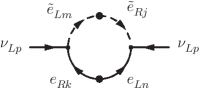
Figure 5: Feynman diagrams generated when, firstly, $\mu_{i}$ induces mixing of interaction state neutrinos with gauginos and higgsinos and secondly, $\lambda_{ijk}\neq 0$ generating neutrino masses radiatively.

For the remaining examples, the bilinear lepton number couplings take the values,

$$\mu_{1}=\frac{\mu_{2}}{\sqrt{2}}=\frac{\mu_{3}}{\sqrt{3}}=1.47\textup{MeV}\;,$$ (4.16)

which reproduce correctly the atmospheric mass squared difference, as shown in Fig. 4. A single, further lepton number violating coupling $\lambda_{ikk}(=-\lambda_{kik})$ is then varied. The branching ratio for lepton flavour violating decays when this coupling correctly generates the observed solar flavour oscillation are calculated numerically using a Fortran code. We find that there are scenarios of this form which correctly reproduce all neutrino data and give rise to branching ratios for $l\rightarrow l^{\prime}\gamma$ which are, or will be, observable in experimental studies.

When $\mu_{1,2,3},\lambda_{ikk}\neq 0$ then diagrams shown in Fig. 5 are generated. It can be seen that the amount of mixing on the fermion line inside the loop, again, corresponds directly to the amount of mixing between interaction state neutrinos and gauginos/higgsinos. It is this mixing which determines the mass of the neutrino produced at tree level and is determined by the values given to the bilinear lepton number violating parameters, $\mu_{i}$. The left hand vertex is determined by the $\lambda$ coupling from the superpotential, as defined in Eq. (1.1). This term in the superpotential generates both couplings in the second diagram of Fig. 5. In fact, if $\lambda_{ikk}\neq 0$, that is, any $\lambda$ coupling with the final two indices the same, a single $\lambda$ coupling will generate this diagram. The branching ratio is approximately given by the following expression,

$$\Gamma(l_{i}\rightarrow l_{j}\gamma)\approx\frac{3}{(4\pi)^{2}}\frac{|\lambda_{ikk}|^{2}}{G_{F}^{2}m_{i}^{2}}\,\frac{e^{2}}{c_{w}^{2}}\,M^{2}_{\chi^{0}}\left[\left(\frac{1}{m_{\tilde{e}}^{2}}\right)\,\left(\frac{\mu_{k}gv_{u}}{M^{2}_{\chi^{0}}}\right)\right]^{2}\Gamma(l_{i}\rightarrow l_{j}\nu_{i}\bar{\nu}_{j})\;.$$ (4.17)

In the following sections, we shall consider in turn all $\lambda$ couplings with symmetric final indices.

4.2.1 $\mu_{1,2,3}$ and $\lambda_{211}$

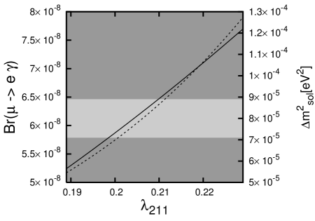
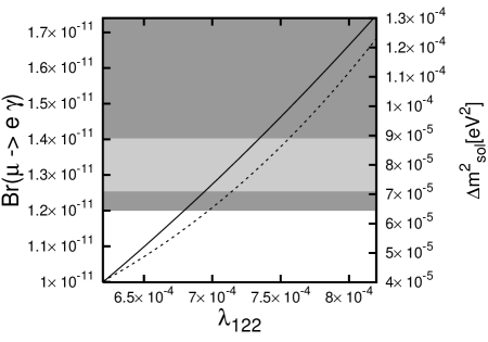
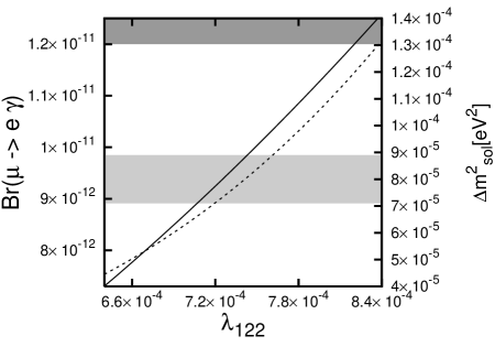
Figure 6: $\mu\rightarrow e\gamma$ and $\Delta m^{2}_{sol}$ against $\lambda_{211}$ or $\lambda_{122}$ – the dotted line (and right hand axis) show the magnitude of $\Delta m^{2}_{\textup{\tiny{sol}}}$ with the light grey band indicating the current $3\sigma$ allowed range; the full line (and left hand axis) show the branching ratio of $\mu\rightarrow e\gamma$ with the dark grey area showing the values currently excluded at 90% confidence level. For the upper two plots, the R-parity conserving parameters are set by the SPS1a benchmark points, for which the mass of the charged scalar that consists mostly of interaction state $\tilde{\mu}_{R}$ is approximately 143 GeV. For the lower two plots, the mass of the scalars was increased such that the mass of $\tilde{\mu}_{R}$ was raised to 145 GeV (bottom left) and 265 GeV (bottom right).

The first example considered is $\lambda_{211}$. As $\lambda_{211}$ is varied, Fig. 6 shows the resulting solar mass squared difference, given by the dashed line, and the $\mu\rightarrow e\gamma$ branching ratio, given by the full line. The light grey strip shows the current experimental value for the solar mass squared difference and the dark grey area is the area presently excluded by $\mu\rightarrow e\gamma$ searches.

The value of $\lambda_{211}$ required to generate the correct value for the solar mass difference must be comparatively large to compensate for the smallness of the mass of the electron induced in the loop. The $\mu\rightarrow e\gamma$ diagram generated has a large mass in the loop, and there is no suppression in the slepton part of the graph due to intergenerational, or left-right, mixing. As such, it can be seen that this scenario, although correctly explaining neutrino masses, is ruled out as it predicts a $\mu\rightarrow e\gamma$ branching ratio which would have been observed already. Furthermore, it is shown in Ref. [33, 34], that a $\lambda_{211}$ coupling of this magnitude would violate charged current universality.

4.2.2 $\mu_{1,2,3}$ and $\lambda_{122}$

In the top right plot of Fig. 6, it is shown that the value of $\lambda_{122}$ required to correctly generate the solar mass squared difference is smaller; a muon is now produced in the loop contributing to the neutrino mass. The lower value of $\lambda_{122}$, in turn, makes the $\mu\rightarrow e\gamma$ branching ratio produced lower than the previous example, however it is still at the edge of the region ruled out by experiment with 90% confidence level. For scenarios with slightly heavier scalar masses than the SPS1a benchmark point this would not be ruled out. In the two bottom plots of Fig. 6 the mass of the scalars has been increased, such that the mass of the charged scalar which is mostly $\tilde{\mu}_{R}$ is 143 GeV (bottom left) and 265 GeV (bottom right) compared to approximately 145 GeV which is produced by the SPS1a benchmark values of R-parity conserving parameters. We note how sensitive the resulting branching ratio is to the mass of the scalar in the loop. As shown in Eq. (4.17), the $\textup{Br}(l\rightarrow l^{\prime}\gamma)\sim 1/m^{4}_{\tilde{\mu}}$. Because this scenario is at the edge of current limits, and because of this sensitivity to the value of scalar masses, it is a particularly interesting scenario which can be studied in future experiments.

4.2.3 $\mu_{1,2,3}$ and $\lambda_{311,133}$

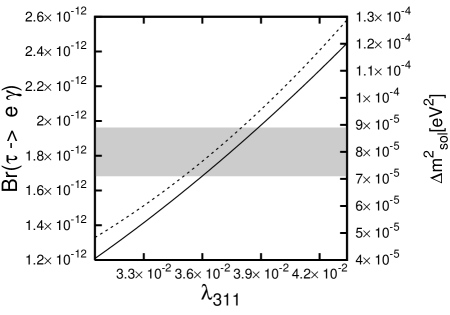
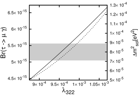
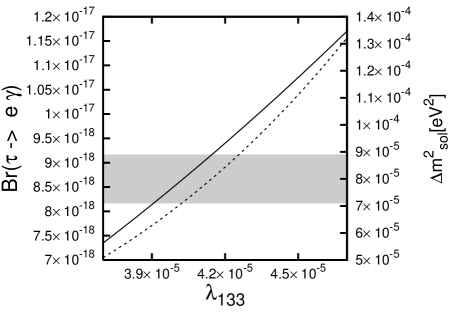
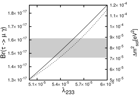
Figure 7: $\tau\rightarrow e\gamma$ (full line, left axis) and $\Delta m^{2}_{sol}$ (dotted line, right axis) against $\lambda_{311,133}$ or $\lambda_{133}$; $\tau\rightarrow\mu\gamma$ (full line, left axis) and $\Delta m^{2}_{sol}$ (dotted line, right axis) against $\lambda_{322}$ or $\lambda_{233}$

In the first plot of Fig. 7, we note the effect on the branching ratio of $\tau\rightarrow e\gamma$ by varying $\lambda_{311}$. The values for $\lambda_{311}$ which correctly reproduce the neutrino data are not ruled out by current rare decay searches. Not only is the experimental bound less stringent, but the branching ratio is suppressed by a factor of $(m_{\tau}^{2}/m_{\mu}^{2})(\textup{Br}(\mu\rightarrow e\nu_{\mu}\bar{\nu}_{e})/\textup{Br}(\tau\rightarrow e\nu_{\tau}\bar{\nu}_{e}))\sim 1600$ compared to the that of Sect. 4.2.1 and the fact that the $\lambda$ coupling itself is smaller. The predicted branching ratio generated by the $\lambda_{133}$ coupling that correctly generates the solar mass squared difference, is even smaller due to the lower value of the coupling.

4.2.4 $\mu_{1,2,3}$ and $\lambda_{322,233}$

The right hand plots of Fig. 7 demonstrate that the values of $\lambda_{322}$ or $\lambda_{233}$ which reproduce the neutrino results are not excluded and well below current experimental sensitivity. We note that the values for $\lambda_{322}$ which produce the neutrino mass are smaller than for $\lambda_{211}$ due to mass of the $\mu$ produced in the loop and $\lambda_{233}$ smaller still.

4.3 Atmospheric scale set by $\mu_{1,2,3}$ – Solar scale set by $\lambda^{\prime}_{ikk}$

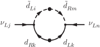
Figure 8: Feynman diagrams generated when $\lambda^{\prime}_{ikk}$ generates neutrino masses radiatively and $\mu_{1,2,3}$ induce mixing on the external leg.

When $\mu_{i},\lambda^{\prime}_{ikk}\neq 0$ the diagrams shown in Fig. 8 are generated. In this case, the mixing on the external leg is driven by the $\mu_{i}$ term, again being determined such that the atmospheric mass difference is produced correctly at tree level. In a similar fashion to the previous section, the $\lambda^{\prime}$ coupling on the left hand vertex is varied and the resulting solar mass squared difference considered. The branching ratio is approximately given by

$$\Gamma(l_{i}\rightarrow l_{j}\gamma)\approx\frac{3}{(4\pi)^{2}}\frac{|\lambda^{\prime}_{ikk}|^{2}}{G_{F}^{2}m_{i}^{2}}\,|(Y_{U})_{kk}|^{2}\,m^{2}_{u_{k}}\left[3\left(\frac{1}{m_{\tilde{d}}^{2}}\right)\left(\frac{\mu_{k}m_{e_{k}}}{m^{2}_{\chi^{\pm}}}\right)\,\left(\frac{{\cal M}^{2}_{\tilde{d}\,LR}}{{\cal M}^{2}_{\tilde{d}\,R}-{\cal M}^{2}_{\tilde{d}\,L}}\right)\right]^{2}\Gamma(l_{i}\rightarrow l_{j}\nu_{i}\bar{\nu}_{j})\;,$$ (4.18)

where ${\cal M}^{2}_{\tilde{d}\,L}$ and ${\cal M}^{2}_{\tilde{d}\,R}$ are diagonal entries in the squark mass matrices and ${\cal M}^{2}_{\tilde{d}\,LR}$ is the off-diagonal term which determines the mixing between the scalar partners of the left and right handed quarks. We note that the mixing between $e_{R}$ and charginos is much smaller than the mixing of $\nu$ and neutralinos, and as such there is a suppression relative to the $\lambda$-driven diagrams. Furthermore, at the SPS1a benchmark point, the squarks are heavier than the charged sleptons; the branching ratios are highly sensitive to the scalar mass and this further suppresses $\lambda^{\prime}$ contributions in comparison with $\lambda$ diagrams. The result being that the $\lambda^{\prime}$ vertices produce a negligible effect in this scenario.

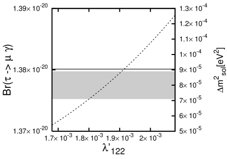
Figure 9: $\tau\rightarrow\mu\gamma$ and $\Delta m^{2}_{sol}$ against $\lambda^{\prime}_{122}$ .

With only the $\mu_{i}\neq 0$, setting the atmospheric mass scale, the diagram shown in Fig. 3 gives a contribution to the $\tau\rightarrow\mu\gamma$ branching ratio of the order $1.38\times 10^{-20}$ (Fig. 4) compared to which we can ignore the contribution from quark loops, as shown in Fig. 9 which takes $\lambda^{\prime}_{122}$ as an example.

4.4 Atmospheric scale set by $\mu_{1,2,3}$ – Solar scale set by $B_{i}$

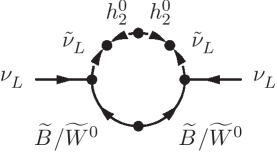
Figure 10: Feynman diagrams generated when the bilinear terms in the superpotential and supersymmetry breaking terms, $\mu_{i}$ and $B_{j}$ respectively, are non-zero

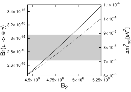
Figure 11: $\tau\rightarrow\mu\gamma$ and $\Delta m^{2}_{sol}$ against $B_{2}$

The diagrams shown in Fig. 10 are generated when $\mu_{i},B_{j}\neq 0$. In the first diagram of Fig. 10, the mixing on the internal fermion is set by $\mu_{j}$ and the mixing on the scalar line is set by $B_{i}$. Again, we note that the mass of the particle inside the loop for the rare decay diagram is of the same order of magnitude as of the particle in the radiative correction to the neutrino mass. The contribution to the branching ratio is approximately given by,

$$\Gamma(l_{i}\rightarrow l_{j}\gamma)\approx\frac{3}{(4\pi)^{2}}\frac{|\lambda_{0jj}|^{2}}{G_{F}^{2}m_{i}^{2}}\frac{e^{2}}{c_{w}^{2}}\;\left[\left(\frac{1}{m^{2}_{H^{+}}}\right)\left(\frac{B_{i}}{m^{2}_{H^{+}}}\right)\left(\frac{\mu_{j}gv_{u}}{m_{\chi^{0}}}\right)\right]^{2}\Gamma(l_{i}\rightarrow l_{j}\nu_{i}\bar{\nu}_{j})\;.$$ (4.19)

As such, we see that these diagrams are not ruled out by current experimental bounds, as shown in Fig. 11, and are not within reach of upcoming studies.

4.5 Atmospheric scale set by $\lambda$ – Solar scale set by $\lambda^{\prime}$

In the following sections, both the atmospheric and solar mass scales are set by radiative corrections. Again, we can find combinations of parameters which correctly describe the neutrino sector and also give rise to experimentally attainable branching ratios for $l\rightarrow l^{\prime}\gamma$.

We first consider the case in which $\lambda_{133}$ and $\lambda_{233}$ are varied over the following range,

$$\lambda_{133}=-\sqrt{2}\lambda_{233}=5\times 10^{-5}-8\times 10^{-5}\;.$$ (4.20)

Figure 12: Feynman diagrams which contribute to $l_{i}\rightarrow l_{j}\gamma$, in the case where trilinear lepton number violating couplings are dominant.

The ratio ensures the correct mixing between neutrino interaction states is reproduced and the magnitude sets in atmospheric masses squared difference. In addition to this, the contribution of the first diagram in Fig. 12 to the branching ratio of $l\rightarrow l^{\prime}\gamma$ is approximately given by,

$$\Gamma(l_{i}\rightarrow l_{j}\gamma)\approx\frac{3}{(4\pi)^{2}}\frac{|\lambda_{ikk}|^{2}\;|\lambda_{jkk}|^{2}}{G_{F}^{2}}\;\left[\frac{1}{24}\frac{1}{m^{2}_{\tilde{\nu}}}\right]^{2}\Gamma(l_{i}\rightarrow l_{j}\nu_{i}\bar{\nu}_{j})\;.$$ (4.21)

The results are given in the upper left panel on Fig. 13. The dashed line (and right hand axis) show the atmospheric mass squared difference and the light grey band shows the values for which $\lambda_{133,233}$ generate an atmospheric mass difference in agreement with current experimental observations. The full line (and left hand axis) show the corresponding branching ratio for $\mu\rightarrow e\gamma$. The resulting branching ratio is well below current or future experimental sensitivity.

To generate the solar mass squared difference, $\lambda_{1kk,2kk,3kk}$ are varied in the following hierarchy, ensuring the resulting mixing matrix takes the form observed by experiment,

$$\lambda^{\prime}_{1kk}=\frac{\lambda^{\prime}_{2kk}}{\sqrt{2}}=-\frac{\lambda^{\prime}_{3kk}}{\sqrt{3}}\;.$$ (4.22)

The second diagram in Fig. 12, produces a contribution to the $l_{i}\rightarrow l_{j}\gamma$ branching ratio of approximately,

$$\Gamma(l_{i}\rightarrow l_{j}\gamma)\approx\frac{3}{(4\pi)^{2}}\frac{|\lambda^{\prime}_{ikk}|^{2}\;|\lambda^{\prime}_{jkk}|^{2}}{G_{F}^{2}}\;\left[\frac{1}{3}\frac{1}{m^{2}_{\tilde{u}}}\right]^{2}\Gamma(l_{i}\rightarrow l_{j}\nu_{i}\bar{\nu}_{j})\;.$$ (4.23)

The results for the three possible cases, that is $k=1,2,3$, are shown in the remaining panels of Fig. 13. We note that while $k=2,3$ are well below current or planned experimental sensitivity, the scenario in which $\lambda^{\prime}_{111,211,311}$ generate the solar mass squared difference would be discernible by upcoming experimental studies, although we note that bounds from $\mu-e$ conversion in nuclei already strongly constrain this set of parameters [35]. When the solar mass squared difference is generated by $\lambda^{\prime}_{133,233,333}$, bottom right panel of Fig. 12, the branching ratio is of the same order as that given by $\lambda_{133,233}$, setting the solar scale, and contributes with opposite sign. Resulting in the negative gradient shown.

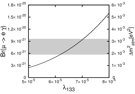
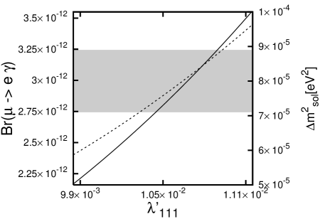
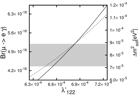
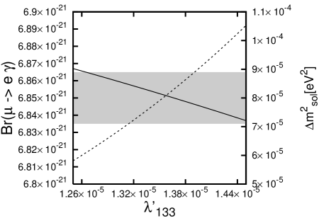
Figure 13: $\mu\rightarrow e\gamma$ and $\Delta m^{2}_{sol,atm}$ against $\lambda^{(^{\prime})}$ – In the top left panel $\lambda_{133,233}$ are varied and the resulting branching ratio for $\mu\rightarrow e\gamma$ (full line, left hand axis) and $\Delta m^{2}_{atm}$ (dashed line, right hand axis, grey band showing current $3\sigma$ band from experiment) are noted. In the remaining three panels, $\lambda^{\prime}_{1kk,2kk,3kk}$ are varied and Br($\mu\rightarrow e\gamma$) and $\Delta m^{2}_{sol}$ are shown.

4.6 Atmospheric scale set by $\lambda^{\prime}$ – Solar scale set by $\lambda^{(^{\prime})}$

Again, both the atmospheric and solar mass scales are set by radiative corrections. First, we consider the scenario in which the atmospheric mass squared difference is set by $\lambda^{\prime}_{111,211,311}$. The parameters are given by,

$$\lambda^{\prime}_{111}=\frac{\lambda^{\prime}_{211}}{\sqrt{2}}=\frac{\lambda^{\prime}_{311}}{\sqrt{3}}\;.$$ (4.24)

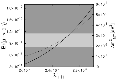
Figure 14: $\mu\rightarrow e\gamma$ and $\Delta m^{2}_{atm}$ against $\lambda^{\prime}_{111}$ – $\lambda^{\prime}_{111,211,311}$ are varied and the resulting branching ratio for $\mu\rightarrow e\gamma$ (full line, left hand axis, dark grey area showing values excluded by experimental searches) and $\Delta m^{2}_{atm}$ (dashed line, right hand axis, light grey band showing current $3\sigma$ band from experiment) are noted.

The resulting atmospheric mass squared difference and resulting branching ratio for $\mu\rightarrow e\gamma$ are shown in Fig. 14, from which it can be seen that the parameter space which brings about the correct atmospheric mass difference is already ruled out by the rare decay searches.

In a similar fashion, we consider the scenario in which the atmospheric mass squared difference is set by $\lambda^{\prime}_{133,233,333}$, as follows,

$$\lambda^{\prime}_{133}=\frac{\lambda^{\prime}_{233}}{\sqrt{2}}=\frac{\lambda^{\prime}_{333}}{\sqrt{3}}\;.$$ (4.25)

The results are given in the upper left panel of Fig. 15. In this case, we note that the values of $\lambda^{\prime}_{133,233,333}$ which give the correct value for the neutrino mass, generate negligible rates for $\mu\rightarrow e\gamma$.

The solar mass squared difference must now be generated. It can be set either by $\lambda_{133,233}$ or by a different set of $\lambda^{\prime}$ couplings. First we examine $\lambda^{\prime}_{1kk,2kk,3kk}$, which are varied as follows,

$$\lambda^{\prime}_{1kk}=\frac{\lambda^{\prime}_{2kk}}{\sqrt{2}}=-\frac{\lambda^{\prime}_{3kk}}{\sqrt{3}}\;.$$ (4.26)

The upper right and bottom left panels show the results for these parameters. Again, we note that although the scenario in which the solar scale is set by $\lambda^{\prime}_{122,222,322}$ (bottom left panel) is not within experimental sensitivity, $\lambda^{\prime}_{111,211,311}$ (top right panel) is close to the current bounds and would be seen by searches planned for the near future.

The final possibility is that the solar mass squared difference be set by $\lambda_{133,233}$. The parameters are varied in the following hierarchy,

$$\lambda_{133}=-\sqrt{2}\lambda_{233}\;.$$ (4.27)

The results, given in the bottom right panel of Fig. 15, show that this scenario is well below both current and future experimental bounds.

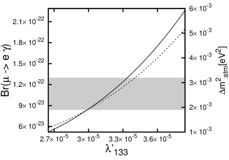
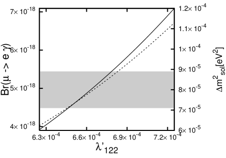
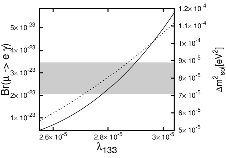
Figure 15: $\mu\rightarrow e\gamma$ and $\Delta m^{2}_{sol,atm}$ against $\lambda^{(^{\prime})}$ – In the top left panel $\lambda^{\prime}_{133,233,333}$ are varied and the resulting branching ratio for $\mu\rightarrow e\gamma$ (full line, left hand axis) and $\Delta m^{2}_{atm}$ (dashed line, right hand axis, grey band showing current $3\sigma$ band from experiment) are noted. In the top right and bottom left panels, $\lambda^{\prime}_{111,211,311}$ and $\lambda^{\prime}_{122,222,322}$ are varied, respectively, and the $\mu\rightarrow e\gamma$ and $\Delta m^{2}_{sol}$ are shown. In the bottom right hand panel $\lambda_{133,233}$ are varied and the $\mu\rightarrow e\gamma$ and $\Delta m^{2}_{sol}$ are given.

5 Benchmarks

Benchmark scenarios for studying R-parity violating models have been suggested [36], for which the mass spectrum, nature of the lightest supersymmetric particle and decays have been studied. The benchmarks presented in [36] are selected as they produce interesting signatures at future colliders and are constrained by measurements of $(g-2)_{\mu}$, the $b\rightarrow s\gamma$ decay and mass bounds from direct particle searches.

In addition to these benchmarks, we suggest some other interesting scenarios. Our motivation being that neutrino data is known and we demand that the model correctly reproduces these results. As there are numerous combinations of lepton number violating parameters which satisfy this requirement, we consider scenarios for which the upcoming $l\rightarrow l^{\prime}\gamma$ searches will constrain the Lagrangian parameters.

The following combinations of lepton number violating parameters are considered, where all R-parity conserving parameters are set at the SPS1a benchmark point,

• Benchmark Scenario 1 –

  $$\mu_{1}=\frac{\mu_{2}}{\sqrt{2}}=\frac{\mu_{3}}{\sqrt{3}}=1.47\textup{MeV}\;\;,\;\;\lambda_{211}=7.4\times 10^{-4}$$

• Benchmark Scenario 2 –

  $$\mu_{1}=\frac{\mu_{2}}{\sqrt{2}}=\frac{\mu_{3}}{\sqrt{3}}=1.47\textup{MeV}\;\;,\;\;\lambda_{311}=3.7\times 10^{-2}$$

• Benchmark Scenario 3 –

  $$\lambda_{133}=-\sqrt{2}\lambda_{233}=6.5\times 10^{-5}\;\;,\;\;\lambda^{\prime}_{111}=\frac{\lambda^{\prime}_{211}}{\sqrt{2}}=-\frac{\lambda^{\prime}_{311}}{\sqrt{3}}=1.05\times 10^{-2}$$

• Benchmark Scenario 4 –

  $$\lambda^{\prime}_{133}=\frac{\lambda^{\prime}_{233}}{\sqrt{2}}=\frac{\lambda^{\prime}_{333}}{\sqrt{3}}=3.25\times 10^{-5}\;\;,\;\;\lambda^{\prime}_{111}=\frac{\lambda^{\prime}_{211}}{\sqrt{2}}=-\frac{\lambda^{\prime}_{311}}{\sqrt{3}}=1.05\times 10^{-2}\;.$$

In the first two benchmark scenarios the observed flavour oscillations of atmospheric neutrinos are driven by the bilinear lepton number violating term in the superpotential giving rise to a mass difference at tree level. For this to occur, the $\mu_{i}$ parameters are of the order 1 MeV. In Benchmark Scenario 1, the solar mass squared difference is then generated by setting $\lambda_{211}=7.4\times 10^{-4}$. Merely for comparison, we note that this is approximately $\lambda_{211}\sim 25\,y_{e}$, where $y_{e}$ is the Yukawa coupling associated with a given particle, in this case being the electron. This will give rise to branching ratios for $\mu\rightarrow e\gamma$ which can be probed by upcoming experimental studies. In Benchmark 2 the solar mass squared difference is determined by $\lambda_{311}=3.7\times 10^{-2}\sim 1200\,y_{e}$. This combination of parameters will generate a branching ratio for $\tau\rightarrow e\gamma$ which may be probed by future studies of $\tau$ decays.

In the Benchmark Scenarios 3 and 4 both the atmospheric and solar mass squared differences are set by radiative corrections. The bilinear lepton number violating terms are set to zero, and the neutrinos are all massless at tree-level. In Benchmark Scenario 3, $|\lambda_{133,233}|\sim 3y_{e}$ set the atmospheric mass difference and $|\lambda^{\prime}_{111,211,311}|\sim 40\,y_{d}$ sets the solar mass squared difference. In Benchmark Scenario 4, $|\lambda^{\prime}_{133,233,333}|\sim 0.1\,y_{d}$ sets the atmospheric scale and $|\lambda^{\prime}_{111,211,311}|\sim 40\,y_{d}$ gives the solar scale. In both Benchmarks 3 and 4, $\mu\rightarrow e\gamma$ would give branching ratios which will be observed by future experimental studies.

6 Conclusions

That lepton flavour violating decays of charged particles have not been observed is worthy of note. The suppressed branching ratios arise automatically in the Standard Model, but this is not the case in Supersymmetric extensions where it already puts strong bounds on certain parameters. In this paper, we have examined the effects of lepton number violating couplings on these branching ratios. Combinations of parameters which describe the neutrino sector were chosen to be examined and their subsequent effect on the rare decays considered.

We first investigated the case in which R-parity conserving parameters are set to the SPS1a benchmark point and the bilinear lepton number violating term in the superpotential, $\mu_{i}$ generates the atmospheric mass difference. We showed that the values of $\mu_{i}$ which correctly describe the atmospheric mass difference and mixing angles are not ruled out by the current bounds on $\tau\rightarrow\mu\gamma$, $e\gamma$ or $\mu\rightarrow e\gamma$. As such, the bounds from lepton decays are less stringent than the bounds from neutrino data. We then considered the case in which a further lepton number violating parameter correctly reproduces the solar mass difference and considered the combined effect on the $l\rightarrow l^{\prime}\gamma$ decays. We note that in this scenario these decays can impose constraints on one of the trilinear lepton number violating parameters in the superpotential, $\lambda$. We considered all the examples in which the $\lambda$ coupling has symmetric final indices, which generate the solar neutrino mass with just one non-zero coupling. $\lambda_{211}$ and $\lambda_{122}$ are excluded by experimental searches for $\mu\rightarrow e\gamma$; $\lambda_{311}$, $\lambda_{133}$, $\lambda_{332}$, $\lambda_{233}$ are not. We note, however, that the branching ratios are sensitive to the masses of the scalar particles in the loop. As such, in scenarios where the scalar masses are heavier than those in SPS1a, the branching ratios can be greatly suppressed.

In this scenario, the limits on $l\rightarrow l^{\prime}\gamma$ do not place useful constraints on $\lambda^{\prime}$, or the bilinear lepton number violating terms in the supersymmetry breaking part of the Lagrangian, $B_{i}$; generally, the current constraints from the neutrino sector are stronger.

Second, we considered the scenario in which trilinear lepton number violating couplings are dominant. We set all bilinear lepton number violating couplings to zero, and again set R-parity conserving parameters to the SPS1a benchmark point. In this scenario, both neutrino mass scales are determined by radiative corrections and in order to generate the correct mixing matrix in the lepton sector, more than one lepton number violating coupling must be non-zero for each mass scale. Because of this, diagrams which contribute to $l\rightarrow l^{\prime}\gamma$ are generated. We note that limits already exist when $\lambda^{\prime}_{111,211,311}$ are used to generate mass differences in this scenario. In general however, for $\lambda^{(^{\prime})}_{x22,x33}$ the constraints from the neutrino masses are stringent.

Acknowledgements

I would like to thank Athanasios Dedes and Janusz Rosiek for their help and support in producing this work. I would also like to acknowledge the award of a PPARC studentship.

Appendix A Appendix

In this section, we present the Feynman Rules for the /L-MSSM. The mixing matrices, $Z$, diagonalise the mass matrices of the model and determine the amount of interaction eigenstate in each mass eigenstate. The full mass matrices and definitions of the mixing matrices are presented in Ref. [13].

A.1 Neutral Scalar - Charged Fermion - Charged Fermion interactions

$\displaystyle-\frac{ie}{s_{W}}\frac{1}{\sqrt{2}}Z_{R1q}Z^{*}_{-1p}Z_{+2r}-\frac{ie}{s_{W}}\frac{1}{\sqrt{2}}Z_{R(2+\alpha)q}Z_{+1r}Z^{*}_{-(2+\alpha)p}$ $\displaystyle+i\lambda^{\phantom{*}}_{\alpha\beta j}\frac{1}{\sqrt{2}}Z_{R(2+\beta)q}Z^{*}_{-(2+\alpha)p}Z_{+(2+j)r}$

$\displaystyle-\frac{e}{s_{W}}\frac{1}{\sqrt{2}}Z_{A1q}Z^{*}_{-1p}Z_{+2r}-\frac{e}{s_{W}}\frac{1}{\sqrt{2}}Z_{A(2+\alpha)q}Z_{+1r}Z^{*}_{-(2+\alpha)p}$ $\displaystyle-\lambda^{\phantom{*}}_{\alpha\beta j}\frac{1}{\sqrt{2}}Z_{A(2+\beta)q}Z^{*}_{-(2+\alpha)p}Z_{+(2+j)r}$

A.2 Charged Scalar - Neutral Fermion - Charged Fermion interactions

$\displaystyle-i\frac{e}{s_{W}}Z_{H(2+\alpha)q}Z^{*}_{-1p}Z_{N(4+\alpha)r}-i\lambda^{\phantom{*}}_{\alpha\beta j}Z_{H(5+j)q}Z^{*}_{-(2+\beta)p}Z_{N(4+\alpha)r}$ $\displaystyle+i\frac{e}{\sqrt{2}c_{W}}Z_{H(2+\alpha)q}Z^{*}_{-(2+\alpha)p}Z_{N1r}+i\frac{e}{\sqrt{2}s_{W}}Z_{H(2+\alpha)q}Z_{N2r}Z^{*}_{-(2+\alpha)p}$

$\displaystyle-i\lambda^{\phantom{*}}_{\alpha\beta j}Z^{*}_{H(2+\beta)q}Z_{+(2+j)p}Z_{N(4+\alpha)r}-i\sqrt{2}\frac{e}{c_{W}}Z^{*}_{H(5+i)q}Z_{+(2+i)p}Z_{N1r}$ $\displaystyle-i\frac{e}{\sqrt{2}c_{W}}Z^{*}_{H1q}Z_{+2p}Z_{N1r}-i\frac{e}{s_{W}}Z^{*}_{H1q}Z_{+1p}Z_{N3r}$ $\displaystyle-i\frac{e}{\sqrt{2}s_{W}}Z^{*}_{H1q}Z_{N2r}Z_{+2p}$

A.3 Squark - Charged Fermion - Quark interactions

$\displaystyle+i{\lambda^{\prime}}^{\phantom{*}}_{\!\!\alpha ij}Z_{\tilde{u}iq}Z^{*}_{-(2+\alpha)p}Z_{d_{R}jk}$

$\displaystyle-i\frac{e}{s_{W}}Z^{*}_{\tilde{u}iq}Z_{+1q}Z^{*}_{d_{L}ij}+i\left(Y_{U}\right)^{\phantom{*}}_{ik}Z^{*}_{\tilde{u}(3+k)q}Z^{*}_{d_{L}ij}Z_{+2q}$

$\displaystyle+i\left(Y_{U}\right)^{\phantom{*}}_{ij}Z^{*}_{\tilde{d}iq}Z^{*}_{u_{R}jk}Z_{+2p}$

$\displaystyle+i{\lambda^{\prime}}^{\phantom{*}}_{\!\!\alpha ij}Z_{\tilde{d}(3+j)q}Z^{*}_{-(2+\alpha)p}Z_{u_{L}ik}-i\frac{e}{s_{W}}Z_{\tilde{d}iq}Z^{*}_{-1p}Z_{u_{L}ik}$

References

- [1] T. Schwetz, Phys. Scripta T127 (2006) 1 [arXiv:hep-ph/0606060].
- [2] T. P. Cheng and L. F. Li, Phys. Rev. Lett. 38 (1977) 381.
- [3] F. Borzumati and A. Masiero, Phys. Rev. Lett. 57 (1986) 961.
- [4] B. de Carlos, J. A. Casas and J. M. Moreno, Phys. Rev. D 53 (1996) 6398 [arXiv:hep-ph/9507377].
- [5] J. Hisano and K. Tobe, Phys. Lett. B 510, 197 (2001) [arXiv:hep-ph/0102315].
- [6] S. Lavignac, I. Masina and C. A. Savoy, Phys. Lett. B 520, 269 (2001) [arXiv:hep-ph/0106245].
- [7] J. A. Casas and A. Ibarra, Nucl. Phys. B 618, 171 (2001) [arXiv:hep-ph/0103065].
- [8] A. de Gouvea, S. Lola and K. Tobe, Phys. Rev. D 63, 035004 (2001) [arXiv:hep-ph/0008085].
- [9] B. de Carlos and P. L. White, Phys. Rev. D 54 (1996) 3427 [arXiv:hep-ph/9602381].
- [10] L. E. Ibanez and G. G. Ross, Nucl. Phys. B 368 (1992) 3.
- [11] H. K. Dreiner, C. Luhn and M. Thormeier, Phys. Rev. D 73 (2006) 075007 [arXiv:hep-ph/0512163].
- [12] B. C. Allanach, A. Dedes and H. K. Dreiner, Phys. Rev. D 69 (2004) 115002 [Erratum-ibid. D 72 (2005) 079902] [arXiv:hep-ph/0309196].
- [13] A. Dedes, S. Rimmer and J. Rosiek, JHEP 0608 (2006) 005 [arXiv:hep-ph/0603225].
- [14] A. Dedes, S. Rimmer, J. Rosiek and M. Schmidt-Sommerfeld, Phys. Lett. B 627 (2005) 161 [arXiv:hep-ph/0506209].
- [15] L. J. Hall and M. Suzuki, Nucl. Phys. B 231 (1984) 419.
- [16] A. S. Joshipura and M. Nowakowski, Phys. Rev. D 51, 2421 (1995) [arXiv:hep-ph/9408224].
- [17] T. Banks, Y. Grossman, E. Nardi and Y. Nir, Phys. Rev. D 52, 5319 (1995) [arXiv:hep-ph/9505248].
- [18] M. Nowakowski and A. Pilaftsis, Nucl. Phys. B 461, 19 (1996) [arXiv:hep-ph/9508271].
- [19] H. K. Dreiner, C. Luhn, H. Murayama and M. Thormeier, arXiv:hep-ph/0610026.
- [20] P. F. Harrison, D. H. Perkins and W. G. Scott, Phys. Lett. B 530, 167 (2002) [arXiv:hep-ph/0202074].
- [21] M. Ahmed et al. [MEGA Collaboration], Phys. Rev. D 65, 112002 (2002) [arXiv:hep-ex/0111030].
- [22] B. Aubert et al. [BABAR Collaboration], Phys. Rev. Lett. 95, 041802 (2005) [arXiv:hep-ex/0502032].
- [23] B. Aubert et al. [BABAR Collaboration], Phys. Rev. Lett. 96 (2006) 041801 [arXiv:hep-ex/0508012].
- [24] Y. Mori et al. [PRISM/PRIME working group], LOI-25 [http://psux1.kek.jp/~jhf-np/LOIlist/LOIlist.html].
- [25] M. A. Giorgi [SuperB group], “SuperB: a High Luminosity Flavour Factory”, [http://www.infn.it/csn1/Roadmap/Super%20B.pdf].
- [26] L. Calibbi, A. Faccia, A. Masiero and S. K. Vempati, arXiv:hep-ph/0605139.
- [27] W. M. Yao et al. [Particle Data Group], J. Phys. G 33 (2006) 1.
- [28] H. Haber, “Practical Methods for treating Majorana fermions”, lecture given at Pre-SUSY 2005, http://www.ippp.dur.ac.uk/pre-SUSY05/ . See also, H.K. Dreiner, H. E. Haber and S. P. Martin, unpublished.
- [29] A. Brignole and A. Rossi, Nucl. Phys. B 701 (2004) 3 [arXiv:hep-ph/0404211].
- [30] A. Dedes, H. Haber and J. Rosiek, in preparation
- [31] B. C. Allanach et al., in Proc. of the APS/DPF/DPB Summer Study on the Future of Particle Physics (Snowmass 2001) ed. N. Graf, Eur. Phys. J. C 25 (2002) 113 [eConf C010630 (2001) P125] [arXiv:hep-ph/0202233].
- [32] D. F. Carvalho, M. E. Gomez and J. C. Romao, Phys. Rev. D 65 (2002) 093013 [arXiv:hep-ph/0202054].
- [33] V. D. Barger, G. F. Giudice and T. Han, Phys. Rev. D 40 (1989) 2987.
- [34] B. C. Allanach, A. Dedes and H. K. Dreiner, Phys. Rev. D 60 (1999) 075014 [arXiv:hep-ph/9906209].
- [35] K. Huitu, J. Maalampi, M. Raidal and A. Santamaria, Phys. Lett. B 430 (1998) 355 [arXiv:hep-ph/9712249].
- [36] B. C. Allanach, M. A. Bernhardt, H. K. Dreiner, C. H. Kom and P. Richardson, arXiv:hep-ph/0609263.